Assortative matching and search

Digitized

by

the

Internet

Archive

in

2011

with

funding

from

Boston

Library

Consortium

Member

Libraries

)

HB31

.M415

working

paper

department

of

economics

ASSORTATIVE MATCHING

AND

SEARCH

RobertShinier Lones Smith No. 97-2 March, 1997

massachusetts

institute

of

technology

50 memorial

drive

Cambridge, mass.

02139

WORKING

PAPER

DEPARTMENT

OF

ECONOMICS

ASSORTATIVE MATCHING

AND

SEARCH

RobertShinier LonesSmith No. 97-2 March, 1997

MASSACHUSETTS

INSTITUTE

OF

TECHNOLOGY

50

MEMORIAL

DRIVE

CAMBRIDGE,

MASS.

021329

i

Assortative

Matching

and

Search*^

Robert

Shimer*

Lones

Smith§

Department

of

Economics

Department

of

Economics

Princeton

University

M.I.T.

February,

1996

Abstract

This

paper

reprises Becker's (1973) neoclassical

marriage

market

model,

assuming

search frictions:

There

is a

continuum

ofheterogeneous agentswith types

xGK;

match

(x,_{y) yields}flow

output

f(x, y)

=

f(y,x),

and

utility is transferable; foregone

output

is the only cost of search.

We

characterize equilibrium

and

constrained efficient matchings,

and

prove equilibrium existence.

We

then

compare

matching

patterns with

Becker's

benchmark

frictionlessallocation,

where

positively ornegatively assortative

matching

arises as agents' types are

complements

or

substi-tutes in production.

We

formalize a notion of assortative-

matching

with

search frictions in the spirit ofaffiliation,

and

demonstrate

that Becker's

condition

no

longer suffices

--

e.g. f(x,y)

=

(x

+

_y)2

produces

highly

nonassortative matching. Fortunately,

we

prove that assortative

match-ing does

extend

to

both

search settings - - _{for all search frictions}

_and

type distributions - -

_under

_{stronger assumptions: supermodularity of}

not just /, but also

log/

x

and \ogf

xy.

Examples

illustrate the

neces-sity ofthese conditions.

We

show

that our assortative

matching

notion

in fact implies that everyone

matches

with a convex set of types; as a biproduct, this

paper

also provides a theory of

convex

matching

sets.

*We

are grateful to Sheldon Chang (M.I.T.

Math

Dept.) for detecting a serious flaw in a key

proof, and forspending the time tooutline afixfor it.

We

wishto thank Daron Acemoglu, Susan

Athey, PeterDiamond, BartLipman, AndreuMasColell, Andrew McLennan, and CharlesWilson

provided useful comments on this paperor its prequel, as well as participants at the

MIT

Theory

Lunch, and seminars at

NYU

and Princeton.

We

have also benefited fromfrequent help received via sci.math. research. Marcos

Chamon

provided valuable simulations assistance.

tThis paper answers questions originally posed in a 1994 version of our

mimeo

"Matching,

Search, and Heterogeneity." Thatunfinished work

now

focuses on a host ofmacrotopics, such as the cross-sectional nature ofsearch inefficiency, and has a more general model in some respects

than this one, which is honed for a micro audience.

*_{e-mail address: shimer@princeton.edu}

1.

INTRODUCTION

In this paper,

we

revisit

what

is arguably the classic insight of the neoclassical

matching

literature

—

when

assortative

matching

arises

—

in a setting with search

frictions.

We

consider a simple

model

of synergistic

matching

inspired

by

Becker's (1973) seminal analysis of the marriage market.

There

is a

continuum

of

hetero-geneous agents with characteristics

x

in _{[0, 1],}

who

can only

produce

in pairs:

The

flow return of a

match

between

agents

x and

y is f(x,y),

where /

is a

symmet-ric production function

--

for instance, f{x,y)

=

xy.

Everyone

is impatient

and

must

search for partners, with potential

matches

arriving at a Poisson

hazard

rate.

Matching

precludes further search.

Everyone

seeks to

maximize

the present value of her future payoffs,

and

we

ask

who

agrees to

match

with

whom

in a

dynamic

steady

state.

Such matching

decisions turn

on

how

the

match

output

is shared.

Smith

(1996) considers

exogenous

sharing rules, as he studies the

model

where

utility is

not transferable

(NTU).

This

paper

instead posits transferable utility (TU).

We

first study search equilibrium

—

the decentralized solution

when

match

out-put is shared according to the

Nash

bargaining rule.

We

provide

what

we

believe to

be

the first general proof of existence ofsuch

an

equilibrium with heterogeneous

types.1 It is of

independent

value, as it parses the logical

argument

into a three

point recipe for application elsewhere -- _{especially the key continuous}

map

from

strategies to

measures

of

unmatched

agents.

There

are externalities in equilibrium,

since search is costly,

and

the decision of

two

agents to

match

precludes others

from

matching

with either.

As

a result, the present value of

output

inthe

economy

is not

maximized.

We

therefore next

examine

the constrained efficient

outcome.

Here, all

matching

decisions are

made

by

a social planner seeking to

maximize

the present value of output, but unable to circumvent the search frictions faced

by

individuals.

The

central

theme

ofthispaper,

and

our

most

innovative contribution, isthat the

equilibrium

and

constrained optimal

matching outcomes

are united

by important

cross-sectional structure.

To

introduce this, recall Becker's

main

insight into the core allocation of a frictionless market: If types are

complementary

to the

match

output (namely, fxy

>

0), then other things equal, agents should

engage

inpositively

assortative matching.

As

usual, search frictions create

temporal matching

rents,

and

thus

an

acceptable

match

need

not

be an

idealone. Still, the ease with

which

Becker

l

derives his result suggests that there

might be

a simple extension ofthis neoclassical

insight to a

model

with search frictions:

Namely,

agents

might be

willing to

match

with all others

who

are not too different

than

themselves. In this paper,

we

first

dispel

any hopes

of such a free lunch. Instead,

we

demonstrate

the negative result

that for

an

open class of

complementarity

production functions, individuals

may

only be willing to

match

with types

who

are quite different.

An

especially salient

example

is afforded

by

the production function f(x,y)

=

(x

+

_y)2.

The

resulting

matching

pattern, depicted in Figure 2 (page 16), is in

no

way

assortative.

Fortunately, all is not lost: Assortative

matching

does extend to a search setting.

We

find a simple

open

subclass of

complementary

production functions for

which

it arises for

any

search frictions or type distributions.

Our

definition of assortative

matching

is also quite natural,

and

essentially asks that

matching

sets

be

affiliated.

For types inR, this asksthat

any two

agreeable

matches can be

severed,

and

then the greater

two

and

lesser

two

types agreeably rematched.

As

testimony to the richness ofthisnotion,

we show

thatit infact impliesthateveryone

matches

with a

convex

set

oftypes in R. This paper therefore also simultaneously provides a theory of convex

matching

sets.

We

consider this

an

interesting application of the

supermodularity

research

program,

2 insofar as

one

must

combine super/sub-modularity

of (2) the

production function (as in Becker)

and

also of (22) its log

marginal

product

log/a,

and

(Hi) log cross partial derivative

logf

xy.

The

lattercondition implies akey single

crossing property of

matching

preferences.

We

use these

assumptions

to prove that

any

individual z has a quasiconcave

match

surplus function s(z,y)

=

_f[z,y)

—

w(z)

—

w(y),

where w(y)

is the type y's

unmatched

optionvalue. This

immediately produces convex matching

sets,

and

then

it is simply a

matter

oforienting

whether

matching

sets are increasing or decreasing

by

Becker's condition (2). In fact, since one's current value is essentially

an

option

on

future surplus, or

w(z)

=

k

_J

max(0,

f(z,y)

—

w(z)

—

w(y))u(y)dy,

where

the

mass

of

unmatched

type-y agents u(y) is unaffected

by

a single agent,

one view

of

our descriptive theory is that it exclusively develops

and

exploits the properties of

such implicit integral equations.

For

an

intuitive overview ofthe quasiconcavity logic, think of

an

economy

with

search frictions so severe that

any

match

is acceptable. Surplus quasiconcavity

entails

comparing

derivatives

_f

y(z,y)

and

w'(y).

The

time cost of search renders

2

_A

w'(y) a multiple

7

<

1 of the expectation over

unmatched

agents

x

of

_f

_y(x,y).

Thus, the slope of z's surplus function is

_f

y(z,y)

—

jE

x

f

y(x,y).

Under

(i), this is

positive for z

=

1,

and

thus l's surplus function is quasiconcave, simply because

/y(l>y)

>

_fy(

x

,y)

>

lIy{

x

iV) f°r a

^

£•

So by

continuity, the frictionless logic of Becker's result carries

through

for 'high' types with search frictions.

But

at the opposite

extreme

2

=

0, this

argument

fails, because

_f

y(0,y)

and

jf

y(x,y) are

incomparable under

(i) alone.

Here

is

where

(ii)

comes

into play, for

it guarantees that

_f

_y(x,y)/f_y(0,y) is nondecreasing in y.

Then

rewriting

_f

y(0,y)

—

jE

x

f

y(x,y)

>

as

1/7

>

E

x(fy(x,

y)/f

y(0,y)),

we

see that 0's surplus function is

increasing for low partners y

and

decreasing for large y, i.e. quasiconcave. Again,

by

continuity, 'low' types have quasiconcave surplus functions

under

(ii).

Finally,

we

use (Hi) to prove a crucial single-crossing property (SCP): For a

given y, if z solves

_f

y(z,y)

=

E

x

f

y(x,y), then

f

y(z,y')

<

E

x

f

y(x,y') for all y'

>

y.

Loosely, this guarantees that everyone iseither a 'high' or 'low' type. For z's surplus function is quasiconcave if her surplus is falling after

any

extremum:

s

y(z,y)

=

implies s

y(z, y')

<

for y'

>

y. Inother words, the marginal

product f

y(z,y) adjusts

proportionately less

than

the marginal value w'(y),

and

so (if everyone matches),

less

than

the expected marginal product, or

_f

y(z,y')/fy(z,y)

<

w'(y')/w'(y)

=

E

x

f

y(x,y')/

E

x

f

y{x,y).

By

the

SCP,

this holds at z,

and

so is true at all z

<

z

by

(ii). Finally,

by

(i), our quasiconcavity premise is false for types z

>

z, as

s

y(z,y)

=

f

y

(z,y)-"/E

x

f

y(x,y)

>

f

y

(z,y)-E

x

f

y(x,y)

=

0, given the definitionofz.

The

only other

paper

that

we

are

aware

that considers

matching

in a

TU

search

model

with ex ante heterogeneity is Sattinger (1995).

That

paper

does not touch

on

our

most

striking findings

--

the link with

models

in the traditional frictionless

matching

literature, as well as existence ofa search equilibrium.

In section 2,

we summarize

the relevant results of the frictionless

matching

lit-erature.

Our

model

with search frictions is described in section 3. In sections 4

and

5,

we

define

and

characterize search equilibria

and

social optima. In section 6,

we

ask

who

matches

with

whom.

We

first derive the conditions that guarantee

con-vex equilibrium

and

optimal

matching

sets.

We

establish the necessity of our

new

conditions with

some

illustrative examples. This sets the stage for us to define

and

explore (both positively

and

negatively) assortative matching. Section 7 establishes the existence ofasteady stateequilibrium.

We

appendicizethe less intuitive proofs.

2.

THE

FRICTIONLESS

MATCHING

MODEL

Consider a frictionless

matching

model,

with

an

atomless

continuum

of agents.

Everyone

in our

economy

is indexed

by

her publicly observable type, a

number

x 6

[0, 1].

An

agent's type is fixed,

and

determines her productivity while

matched.

Normalize

the

mass

of agents to unity,

and

let the distribution of types

be

L

:

[0,1] i-> [0,1].

The

fraction/mass of agents with type at

most

y is L(y).

We

assume throughout

that

L

is differentiable, with Borel

measurable

type density I.

The

existence proof alone also requires that I

be boundedly

finite

and

positive:

<

L

<

£{

x

)

<

^

<

oo for all x.

One

view ofour set-up is that there is implicitly a

continuum

ofevery type ofagent, with individualsbelonging to the

graph

{(x, i)\x

G

[0, 1],

<

i

<

£{x)},

where

i is

an

index

number

of the type

x

agent.

When

two

individuals oftypes

x

and

y

—

agents

x

and

y

—

are

matched

together,

they

produce

a flow

output

that is purely a function of their types,

/

: _{[0, l]}

2

i-> R.

We

shall later

need

to refer collectively to a set of assumptions:

AO

(Regularity

Conditions). The

-productionfunction

f

is strictly increasing

and

strictlypositive

when

x,y

>

0. It is also symmetric, or f(x,y)

=

f(y,x), continuous,

and

twice differentiable with a uniformly

bounded

first partial derivative.

3

Thus,

everyone prefers to

be

matched

with

someone

rather

than

to

be unmatched,

and, everything else equal, prefers to be

matched

with higher types of agents. In the core allocation,

wages

allocate the scarce resource,

namely

high

produc-tivity agents.

When

does positively assortative

matching

or self-preference obtain,

where

everyone

matches

exclusively with others ofthe

same

type?

A

sufficient

con-dition is that characteristics

be

complementary

inputs in the production function:

Al-Sup

(Strict

Supermodularity).

The

own

marginal product of

any

agent

x

>

is strictly increasing in her partner's type. Equivalently, the production function f is strictly

supermodular

in the positive quadrant:

_f

xy{x,y)

>

when

x,y

>

0.

If

Al-Sup

obtains, then high productivity agents enjoy the highest

marginal

product

when

they are

matched

with other high productivity agents. In the core

allocation,

matching

must

be

(almost surely) positively assortative.

To

see this,

simply note that

any

allocation in

which

some

positive

measure

ofagents oftype

x

match

with agentsof_{type y}

^

x admits

a simple

Pareto-improvement.

If

we

reassign 3

all such agents to another of her

own

type,

output

rises, since _f(x,x)

+

_f(y,y)

>

2f(x,y)

whenever x

^

y given

Al-Sup.

So

the unique value-maximizing allocation

entails assortative matching, with everyone just

matching

with his

own

type.

Constructing

an

equilibriumwith positively assortative

matching

provides a

use-ful

benchmark

for the

remainder

of this paper.

With

a

market

'wage' w°(x) for

every type x,

symmetry

requires that each agent receive half of the

output

from

her match: w°(x)

=

f(x,x)/2.4

We

define for later use the surplus function for x:

s°(x,y)

=

f(x,y)

—

w°(x)

—

w°(y)

measures

how much

the output of a partnership with y exceeds the

sum

ofthe

wages

of the

two

partners. If this is negative for all

x

j^ y, then

we

have constructed

market wages

to decentralize this allocation.

For a given x,

an

increase in her partner's type yields marginal surplus equal to

4(

x

> y)

=

fy(

x

>y)

_

f*(y>y)/2

~

fv(y>y)l2

=

A(

x

'y)

-

fv(y> y)

since / is symmetric. If

Al-Sup

obtains, then

_f

_y(x,y)

_^

_f

y{y,y) as

x

^

y, i.e. for a

given x, the surplus function is increasing or decreasing in her partner's type y as

x

_^

y.

So

it is strictly quasi-concave, with

maximum

value

when

matched

with

a like partner x. Hence,

under

Al-Sup,

the unique equilibrium of this

model

has

positively assortative matching,

and

coincides with the socially optimal allocation.

A

symmetric

result obtains in thefrictionless

matching

model

when

the marginal productivity of

an

agent is a decreasing function of her partner's type.

Al-Sub

(Strict

Submodularity).

An

agent's

own

marginal product is decreasing

in her partner's type. Or, the production function

_f

is strictly submodular:

_f

xy

<

0.

Under

Al-Sub,

the social

optimum

and

unique core allocation entails negatively assortative matching:

Each

agent

x matches

with her 'opposite' type y(x),

where

L(x)

+

L(y(x))

=

1. For

by Al-Sub, f(x

1,y2)

+

f(x

2,yi)

>

f(xi,yi)

+

/(ar_{2 ,I/a)}

whenever

x\

<

x

2

and

y\

<

y

2. It follows that if there are four agents, z\

<

z₂

<

zj,

<

Z4, the allocation in

which

z\

and

z$ are

matched and

z2

and

z$ are

matched,

Pareto

dominates

the

two

otherpossible allocationsin

which

these four agents

match

in pairs.

As

before,

we

can prove the existence of the required core allocation

by

demonstrating

that the surplus function for each agent

x

is a strictly quasi-concave

function of her partner's type, achieving its

maximum

when

her partner is y(x).

Remark

1.

Throughout

the paper,

we

shall generally

maintain

either

Al-Sup

or

Al-Sub.

This excludes, for instance, the knife-edge case of additivity,

where

the

own

marginal product

of

an

agent is

independent

of her partner's type, f(x,y)

=

p(

x

) _(-_g(y):

and

for

which any

allocation

is efficient. Also excluded are production

functions for

which

own

marginal product

is not

monotonic

in partner's type

—

for

example, f(x,y)

=

max(x

2y,

xy

2

)

--as

Kremer

and

Maskin

(1995) exploit.

5

3.

A

MODEL

OF

MATCHING WITH

SEARCH

In this section,

we

develop a continuous time, infinite horizon

model

of

matching

with search frictions.

As

per usual, frictions

mean

that finding

and meeting

other agents is

time-consuming

process.

6

Crucially, with

an

atomless

continuum

ofagents,

if agent

x

uses a rule like 'only

match

with a type y agent', then she will almost

surely never

match.

Rather, everyone

must

be

willing to

match

with

sets of agents.

*

Action

Sets.

At any

instant in continuous time, one is either

matched

or

unmatched.

Only

the

unmatched

engage

in (costless) search for a

new

partner.

When

two

unmatched

agents meet, their types are perfectly observable to each

other. Either

may

veto the

proposed match.

If

both

approve, it is

consummated

and

remains

so until nature destroys the

match.

This event occurs with a constant

flow probability5

>

0, i.e. after

an

elapse time oft with chance e~

St

.

At

the

moment

the

match

is destroyed,

both

agents instantaneously re-enter the pool of searchers.

Remark

2. In steady state, a

match

that is profitable to accept is profitable to

sustain; therefore, to simplify our analysis,

we

disallow

match

quits.

Remark

3.

Match

dissolutions is one

way

to

maintain

asteady-state.

One

could

instead

assume

an

inflow of entrants,

and

that

matches

are eternal.

Our

choice is

moot

for the descriptive theory, but is standard in the

TU

matching

literature.

*

Preferences.

Agents

maximize

their lifetime expected present discounted

payoffs, using the interest rate r

>

0.

We

assume

transferable utility (in a sense

specified later), as the

benchmark

frictionless

model

Becker (1973) is

TU

and

not

5

For such production functions, matching sets are not convex; some agent

may

be willing to

match either _{with y}x or y3, yet unwilling to pair up with y2 G (2/1,2/3)- This provides a

foretaste of section6, where weestablish that convexity and assortative matching are kindred concepts.

6

NTU.

As

such, the flow

income

of

x

when

matched

with y

comes from an

endoge-nously

determined

payoff ix(x\y).

These

payoffs derive

from

the

output

of a match,

so that ir(x\y)

+

7r(y|x)

=

f(x,y) for all

x

and

y.

Unmatched

agents earn nothing.

*

Unmatched

Agents

and

Search.

Let

u

<

£

be

the

unmatched

density function, i.e.

_J

x

u(x)dx

is the

mass

of

unmatched

agents with types

x G

X

C

[0, 1].

Our

search frictions are captured

by

the followingsimple story.

Were

it possible,

an

unmatched

individual

would

meet

another

unmatched

or

matched

agent accord-ing to a Poisson process with constant rendezvous rate

_p

>

0.

But

it is

presumed

technically infeasible to

meet

someone

who

is already

matched

--or

equivalently, the other individual is already engaged,

and

so misses

any

meeting. Thus, the flow probability that agent

x meets any

|/e7C

[0, 1] is _p

_f

y

u(y)dy.

Simply

put, the

rate at

which

one

meets

others with types in

any

subset

Y

is in direct proportion to the

mass

of those

unmatched

in

Y.

Our

cross-sectional results extend well

beyond

this (quadratic) search technology, as

we

underscore in section 8.

*

Strategies.

A

steady state strategy

A(x)

for agent x

G

[0, 1] specifies a Borel

measurable

set of agents with

whom

x

is willing to match.7

(That

all agents of the

same

type

employ

the

same

strategy follows

from

our later analysis.) In the steady

state ofthis model,

A

is time-invariant8

and depends

only

on

the

unmatched

density function u, the payoff-relevant state variable.

Next

define

an

agent's

matching

set,

M(x)

=

A(x)D{y

|

x G

A(y)}, thesetoftypes y with

whom

x

iswillingto

match,

and

who

are willing to

match

with x.

A

match

(x,_y) is mutually agreeable iff _y

G

M(x)

(and so

by symmetry,

iff

x

G

M(y)).

We

also identify each

matching

set with its

match

indicatorfunction a: a(x,_y)

=

1 ify

G

M.(x)

and

otherwise.

*

Steady

State. In steady state, the flow creation

and

flow destruction of

matches

for every type of agent

must

exactly balance.

The

density of

matched

agents

x G

[0,1] is i(x)

—

u(x); these agents'

matches

exogenously dissolve with

flow probability 5.

The

flow of

matches

created

by

unmatched

agents of type

x

is

pu(x)

_f

_M

(x)

u(y) dy. Putting this together, in steady state for

any

type

x G

[0, 1],

5{l(x)

-

u(x))

=

pu(x)

_/

M(x) u(y)

dy

=

pu(x)/„* a(x, y)u(y)

dy

(1)

7

_We

can express strategies as acceptance sets given an atomless type distribution. With type

atoms, equilibrium existence demands mixedstrategies: either probabilistic matching or quitting.

8

_WLOG,

we restrict attention to stationary acceptance sets. Since no single agent can affect

any future state oftheeconomy through her choices, ifanalternative acceptanceset is optimal at

4.

THE

DECENTRALIZED

ECONOMY

We

now

characterize the steady state search equilibria (SE) of this model. Search equilibrium requires that (i) everyone

maximizes

her present discounted payoffs,

taking allotherstrategies as given,

and

(ii) a

match

is

consummated

iff

both

parties

accept it.

Yet

this criterion has insufficient cutting power. For example, ifeveryone

chooses to

match

with

no

one, then

no one

has a strict incentive to deviate. This

outcome

does not

seem

sensible to us, as it doesn't survive the possibility of small

strategy 'trembles'

by

others.

So

we

also insist that everyone also choose a best

response to

any

possible strategy

one might

face at

any

moment.

Equivalently, (ii 1

)

in a

SE

all

matches

with strictly positive

mutual

gains are accepted.

4.1

Search

Equilibrium

•

Value

Equations.

Let

w(x)

denote the expected average present value for

an

unmatched

agent x,

assuming x maximizes

her expected present value.9 Similarly,

let w(x\y)

be

the expected average present value for

x

while

matched

with y.

We

solve for a

SE

by

defining the implicit equations solved

by

these

Bellman

values.

While unmatched, x

earns nothing, but at flow rate _p

J"

M

-(i) u(y)cfa/, she

meets

and

matches

with

some

y

€

M(x),

enjoying a capital gain (w(x\y)

-

w(x))jr.

, x f w(x\y)

—

w(x)

. . , ,n.

w{x)

=

_p

-±-^

—u(y)dy

(2)

JM(x) r

Similarly,

x

enjoys a flow payoff 7r(a;|y)

when

matched

with y.

With

flow probability

5, her

match

is destroyed,

and

she suffers a capital loss (w(x\y)

—

w(x)) jr. Hence,

w

(x\y)

=

n(x\y)

-

S(w{x\y)

-

w{x))/r

(3)

We

can eliminate w(x\y)

from

equations (2)

and

(3),

and

obtain a simple expression

for

w(x)

as a function ofthe equilibrium payoffs tt(x\-).

/ X f n(

X

\y)

—

W

(

X

) I \ 7 (A\

w(x)=p

, x

'

u(y)dy

₍₄₎

The

average

unmatched

value of

x

equals the rate that

x

finds

matches

times the 9

expected discounted present value of the capital gain over her

unmatched

value

-where

discounting incorporates

both

impatience

and

match

impermanence.

*

Acceptance

Sets. In a SE, one accepts

any

match

that increases one's

expected present value. (

w(x\y)

^

w(x)

=> I (5)

(y<£A(x)

In the borderline case w(x\y)

=

w(x), y

G A(x)

is neither necessary nor precluded. -k

Wage

Determination.

Search frictions create

temporal

bilateral

monopoly,

since

match

output

less the agents' outside options (i.e. their

unmatched

values), is

generally positive:

match

surplus s(x,y)

=

f(x,y)

—

w(x)

—

w(y)

>

0. This shifts

the question of

wage

determination into the

realm

ofbargaining theory.

We

abstain

from

innovating

on

this front,

and

simplyfollow a

number

ofauthors,

more

recently Pissarides (1990), in

assuming

the

Nash

bargaining solution,10 i.e. the

instantaneous

match

surplus

--

the excess of

wages

over average

unmatched

values

(w(x\y)

+

w(y\x))

-

(w(x)

+

w(y))

—

is divided equally.

The

wage

schedule satisfies

w(x\y)

-

w(x)

=

w(y\x)

-

w{y)

(6)

So

by

the optimality condition (5), this yields y

G A(x)

iff

x E

A(y), except possibly

in the borderline case w(x\y)

—

w(x)

=

w(y\x)

-

w(y)

=

0.

By

definition,

A(x) and

M(x)

coincide, except possibly in this borderline case.

The

definition ofw{x\y)

from

asset value equation (3)

and

the

Nash

bargaining

schedule (6) yield

7r(x\y)

-

w(x)

=

ir(y\x)

-

w(y)

(7)

Since the payoffs

must

somehow

divide the

output

ofthe

match,

Tr(x\y)

+

7r(y|x)

=

f(x,y),

and

so (7) yields the equivalent

Nash

bargaining payoff schedule:

n(x\y)

=

w{x)

+

\(f{x,y)

-

w(x)

-

w(y)) (8)

In other words, the flow payoff for

an

agent

x

is equal to her flow value

from

being

unmatched

plus half the flow surplus

produced by

the match.

• Synthesis.

To

describethe equilibrium, observethat (3) implies thatw(x\y)

^

w(x)

as Tr(x\y)

_^

w(x), while (8) says n(x\y)

^

w(x)

as f{x,y)

—

w(x)

—

w(y)

^

0.

10

0.6

0.4

0.2

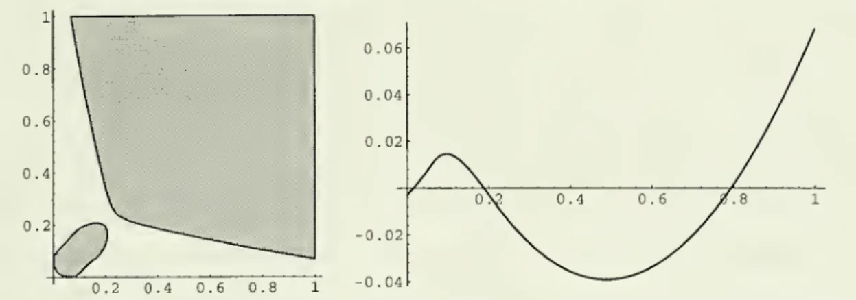
Figure 1:

Equilibrium

Matching

Sets. This depicts the equilibrium matching sets for

f(x,y)

=

xy, with p

—

50r, 5

=

r/2, and a uniform distribution of agents. If x e M(y) and

y e M(x), then the point (x,y) is shaded in the graph.

Combining

this

with

(5) yields the

mutual

optimality condition.

f(x,y)

-w(x) -w{y)

^

y

e

M(x)

y

£

M(x)

(9)

where

we

have used the fact that y

e A(x)

and

x € A(y)

implies y

e M(x).

Next, substituting (8) into (4) yields

an

implicit

system

for

unmatched

values:

f(x,y)

-w(x) -w(y)

w(x)

=

_p

M(x)

2(r

+

5)

u(y)

dy

(10)

Note

that equation (10) is well-defined, even

though

we

have not specified

whether

y

G

M(x) when

f(x, y)

—

w(x)

—

w(y)

=

0.

A

SE

may

intuitively

be

fully described

by

specifying: (i)

who

is

matching

with

whom

(the

matching

sets

M);

(ii) the

mass

of each type searching (the

unmatched

density it);

and

(Hi)

how much

everyone's time is

worth

(the

unmatched

value w).

Proposition

1

(SE

Characterization).

A

SE

can be represented as a triple

(w,M,u)

where:

w

solves the implicit

system

(10), given

(M,

it);

M

meets the

opti-mality condition (9) given

w;

and

u

solves the steady state equation (1) given

M.

Example.

Figure 1 graphically depicts the equilibrium

matching

sets for the

production function _f(x,y)

=

xy

as well as a particular choice of search frictions,

impatience,

and

type distribution. Since this production function satisfies

Al-Sup,

in the frictionless

benchmark

agents are only willing to

match

with their

own

type,

M(x)

=

{x}.

As

one

might

expect, with search frictions, everyone is willing to

accept a rangeof possible partners. In section 6

we

find conditions

on

the production

function that ensure equilibrium

matching

sets have approximately this shape.

4.2

Properties

of

the

Value Function

Before proceeding,

we must

first derive

some

basic properties of the value function.

Our

analysis

throughout

the

paper

repeatedly applies the following inequality:

Observation.

For

any

agent

x and any

set

M

C

[0. 1],

•»(*)

>

p

/

u

j^j

}

*(v)

dy

(ID

Ifthis were not true, then the implicit equation (10)

would

yield ay such that either (?) y

e M(x),

y

£

M.

and

f(x.y)

-

w(x)

-

w(y)

<

0, or (tt) _y

_{i M(x),}

_y

G

M,

and

f(x,y)

—

w(x)

—

w(y)

>

0. Either possibility contradicts (9). This leads us to

Lemma

1

(Monotonicity).

Given

A0. the value

w

>

is

mcreasing

in a SE.

Intuitively, since higher agents are always

more

productive

than

lower agents, they

can simply imitate the

matching

decision of lower agents

and do

better. If they

optimize, they will

do

stillbetter.

The

appendicized proofformalizesthis

argument.

The

logic underlying monotonicity also buttresses continuity:

Anyone

can

do

almost as well as a slightly

more

productive agent, simply

by

imitatingher

matching

decision. Consequently, the value function cannot

jump,

as proven in the appendix.

Lemma

2

(Continuity).

Given

A0

; the valuefunction

w

is continuous in a SE.

U

We

oftenreferto the derivative of the

unmatched

value function. Thisisjustified:

Lemma

3 (Differentiability).

Given

A0, the value function

w

is a.e.

differen-tiable in a SE,

and

its derivative is a.e. given by:

,

M

pki{

X)

U

x

_^)<y)

d

_y . .

W{X)

2(r

+ S)+pJ

M{x)

u(y)dy

[

^

Monotonic

functions are a.e. differentiable,

and

so the first part of the claim follows

from

Lemma

1.

When

the

matching

set is (suitably) differentiable in x, the resulting

formula for w'(x) is a straightforward application of the

Fundamental

Theorem

of 11

Theappendicized proofactually establishes that

w

is Lipschitz.

Calculus: surplus vanishes all along the

boundary

of the

matching

set; therefore,

we

can

safely ignore the effect

on

w'(x) ofchanges in the

matching

set,

and

simply

differentiate (10)

under

the integral sign.

The

difficult appendicized proofcarefully

argues that (i) this logic is stillvalid

when

matching

sets are

merely

continuous

and

the value function Lipschitz at x.

and

{ii)

both

these conditions hold a.e. in x.

Using

these

lemmata,

existence of

SE

is proved. For expositional ease,

and

as it is

an important

inits

own

right,

we

defer analysis ofthis

complex

issue to section 7.

5.

CONSTRAINED

EFFICIENT

MATCHING

In this section,

we

investigate

dynamic

steady states

where matching

decisions are

constrained efficient:

Everyone matches

so as to

maximize

the global present

dis-counted

value of output, rather

than

her

own

personal value. It helps to introduce

a hypothetical social planner

who

is entrusted

with

all

matching

decisions.

True

to

our stated goal,

we

assume

that the planner

cannot

bypass the search frictionsthat render

matching

opportunities infrequent.

We

look for a stationary social

optimum

(SO), the steady state ofthe

optimal

dynamic program

of a constrained planner.12

We

characterize necessary conditions for a

SO,

by

considering only stationary

deviations

from

steadystates.

That

is.

we

do

not allow the planner ii) to destroy

ex-isting matches, or (ii) to

employ

nonstationary

match

acceptance strategies.

These

provisos are required

by

our

model and

strategy space,

and

reflect our steady-state

spirit.

But

they sidestep a very

deep

issue: It is theoretically possible, if

hard

to

fathom, that for

any

initial condition, a nonstationary policy

may

beat

any

station-ary

one

the planner could devise.

To

establish a steady state SE.

we

safely ignored nonstationary deviations, as

no

single agent could affect the future course of the

decentralized

economy;

since a social planner

most

certainly

can

affect the future, this is

no

longer

WLOG,

and

stationary

SO

existence is

much

more

problematic.

13

Let

M*(x)

denote the set ofall agents

whom

the social planner lets

match

with

agent x.

By

construction, y

G M*(x)

iff

x

e

M*(y).

We

will call M*(-)

an

agent's

optimal

matching

set.

and

let a*

be

itsindicator function:

a*

(or,_y)

=

1 iffa:

G

M*(y).

12_This

is analogous to the modified golden rule in theeconomic growth literature.

The

golden

rule, by way of contrast, is the planner's best steady stateifshe can, atan initialtime, costlessly

jump

to her prefered steady state, at which she must remain.

The

two notions coincide for an

infinitelypatient planner (r

=

0),since thetransitionpathis costless.

13

Shimer and Smith (1996) will address

SO

existence allowingforall dynamic strategies.

Let

m

: _{[0, l]}

2

h->

M+

be the density ofmatches, so that

_J

5

m(x,

y) is the

mass

of

matches

for (x,y)

£

S. This satisfies a steady state constraint:

6m(x,y)

=

pa*{x,y)u(x)u(y)

₍₁₃₎

In steady state, the flow dissolution of

matches

(x,y)

must

equal the flow creation

of such matches.

Then,

being careful not to double-count output, the steady state

average present value of

output

in the

economy

is

_J

Q

J

Q \f(x,

y)m(x,

y)dxdy.

Thus

a pair (M*,

m)

is a

SO

only ifthe

matching

sets

M*

maximize

the present value of

output

among

stationary

matching

rules, given the initial

matched

rates

m; and

M*

implies that the state of the

economy

remains

at

m.

We

can think

of the planner

maximizing

the present value of output, subject to the steady state relationship (13).

To

solve for a

SO,

we

could write the planner's

problem

as a Lagrangian, insert e-variations

on

the state variables

m

E

=

m

+

efh, differentiate

with respect to e,

and

reach (a la calculus of variations) a pointwise conclusion given

the arbitrary nature of fa.

We

instead recast this as a current-valued Hamiltonian:

^=-1

I

f(x,y)m(x,y)+p(x,y)(pa(x,y)u(x)u(y)-6m(x,y))dxdy

(14)

^ Jo Jo

where

p(x,y)/2 is the multiplier

on

the steady state relationship (13), half the

planner's value of a

match

(x,y) (again not double-counting).

We

describe the

necessary first order conditions using the notational shortcuts 3ia(x,y)

and

3im(x,y)-The

first condition, a short-cut to placing multipliers

on

the constraint that

a(x,y)

€

[0,1], reflects the

Kuhn-Tucker

complementary

slackness requirements.

14 p(x,_y)

_^

^

M

_a(s ,y)

^0^1

~ (15)

[a(x,y)

=

Inthis 'bang-bang' control,

when

the

shadow

value ofa

match

of

x

with y ispositive,

the planner will

match

them;

when

the

shadow

value is negative, she won't.

The

other (steady state) first order condition determinesp: 3i

m

(x,y)

=

2rP(

x

'

v)-As

the density of

unmatched

agents

x

is u(x)

=

£(x)

—

_J

Q

m(x,

z) dz,

we

have

2M

m

(x,y)

=

f(x,y)

-

5p(x,y)

-

_{p J*} (a(x, z)p(x,z)

+

a(y, z)p{y, z))u{z) dz (16)

14

Optimality onlyrequiresthat the

FOC

hold almost everywhere.

We

assumethey alwayshold.

Let v(x)

=

_p

_f

_M

,(x)p(x, z)u(z)dz

=

p

f

a(x, z)p(x, z)u(z)dz.

As

p(x,z) is the

plan-ner's value ofa

match

(x, z),

we

interpret v(x) as the social

unmatched

value ofagent

x

—

namely, theflow rate at

which

she creates

new

social present value.

Combining

this with 2IK

_m

(x,y)

=

rp(x,y)

and

(16) yields:

p(x,y)

=

(f{x, y)

-v{x)-

v(y))/(r

+

6) (17)

Therefore,

we

can

rewrite condition (15) as

(xeM*{y)

_, x

f(x,y)-v{x)-v(y)%0=>{

(18)

[x$M*{y)

Combining

(17) with the definition of v yields

an

implicit equation for the social

unmatched

value:

v{x)

=

_p

—

—

-:

u{y)dy

(19)

Jm*(i) r

+

o

Proposition

2

(SO

Characterization).

A SO

can be represented as

(v,M*,u)

where: v solves the implicit

system

(19), given

(M*,u);

M*

meets

the optimality

condition (18) given v;

and u

solves the steady state equation (1) given

M*

.

Remark

4.

A

triple (v,

M*,

u) solving (1), (18),

and

(19) is not necessarily a

SO.

It

may

be

dominated

by

nonstationary paths; or it

may

be

a local, but not a global,

maximum

of the planner's problem.

Remark

5. Replacingr

by

2f

+

<5 leaves (18)-(19) identical to (9)-(10), with the

same

steady-state equation (l).15

Then

v

must

share the key properties of w:

Lemma

4

(Value

Properties).

The

social

unmatched

value v is nonnegative,

strictly increasing, continuous,

and

a.e. differentiable, with derivative a.e. given by

v'{x)

r

+

S

+

_pf

_M

,

{x)

u{y)dy

Also,

we

can prove the existence of a triple solving (1), (18),

and

(19). This

follows

from

existence of a

SE

(Proposition 5,

page

27).

However,

this does not

establish existence of a

SO,

as explained in

Remark

4 above.

15_While

this

may

admit f

<

0,

SE

in fact only requires thatf

+

5

>

0, which is still true.

6.

DESCRIPTIVE

THEORY

As

seen insection 2, supermodularity

(Al-Sup)

alone ensures that there ispositively assortative

matching

without search frictions in the core allocation/social

optimum

- _agent

_x

_always

matches

with another agent x. Moreover, the surplus loss

from

not

matching

with one's ideal partner is increasing in the

mismatch:

If

x

<

y

<

z,

then

x

strictly prefers a

match

with y over z. In the frictional setting, everyone still

has

an

ideal partner, but since individuals are willing to

match

with sets of agents,

mismatch

is the rule in equilibrium or at a constrained

optimum.

Curiously, the

form

that this

mismatch

takes is quite unpredictable. For example,

x

may

prefer to

match

with z rather

than

with y

G

(x, z)

—

and sometimes would

rather

match

with

z

than

with another x\ This significant violation of positive assortative

matching

motivates our

new

conditions

on

the production function.

Remark

6.

Throughout

this section

we

simply refer to properties of

matching

sets

—

as they are equally true of

any

SE

or

SO.

For indeed,

both

SE

and

SO

have

identical value properties,

which

drive all results reported here.

But

for brevity

and

clarity, our language

and

notation pertain to SE.

Note

that while search equilibrium

depends on

the exact specification of

how

surplus is divided within a

match,

SO

does

not suffer

from

this ambiguity. This section nonetheless unites these

two

disparate

concepts,

which

serves as a further robustness check

on

our descriptive theory.

6.1

Convexity

First

on

our

agenda

is convexity: If

x

is willing to

match

with y\

and

y3, will she

also agree to

match

_{with y}2

6

(2/1,2/3)? Optimality condition (9) tells us that if x's surplus function s(x,y)

=

f(x,y)

—

w(x)

—

w(y)

is strictly quasiconcave in _y,

then the

answer

to this question is 'yes'.16 Section 2 proved that

Al-Sup

or

Al-Sub

ensures a quasiconcave surplus function in the frictionless

benchmark

model.

Example.

Surprisingly, neither

Al-Sup

nor

Al-Sub

suffices with search

fric-tions.

With

the

supermodular

production function f(x,y)

=

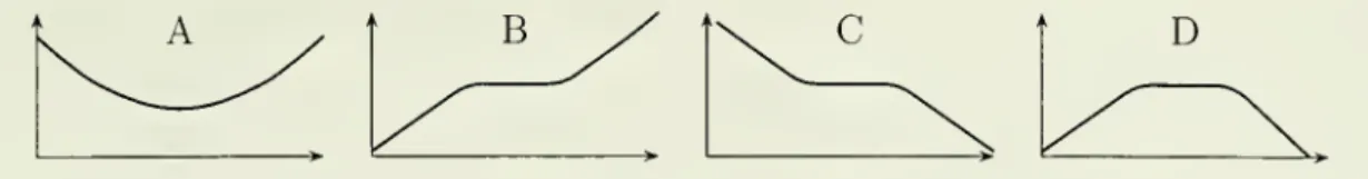
(x

+

_y)2 in Figure 2,

there is positively assortative

matching

in the frictionless case.

But

with search

frictions, equilibrium

matching

sets are not convex. Indeed,

any x £

(0.20, 0.21)

won't

match

with her

own

type, but will

match

both

with higher

and

lower types. 16

Ofcourse, convexity

may

obtainevenifthe surplusfunction is not quasiconcave; however,we

see no general proofofconvexity that does not rely on quasiconcavity.

0.2 0.4 0.06 0.04 0.02 -0.02 -0.04

Figure 2:

Non-Convex

Matching and

Nonquasiconcave

Surplus Function.

The left panel depicts the equilibrium matching sets for f(x,y)

=

(x

+

_y)2, with p

=

40r, S

=

r/2,

and a uniform distribution of types. All points (x,y) with y £ M(x) are shaded in the graph.

The equilibrium matching sets ofany x £ (0.07,0.21) are not convex. The right panel depicts the

non-quasiconcaveflow surplus s(0.1,j/) for all matcheswith agent 0.1.

Also,

when

f(x,y)

=

(x

+

_y)2, everyone has a strictly (quasi-)concave surplus

function in the frictionless

benchmark,

with

maximum

surplus

when

each type

x

matches

with another x. Indeed, the

wage

is w°(x)

=

2x

2

and

surplus s°(x,y)

=

—

(x

—

_y)2.

One

might imagine

that search frictions simply reduce everyone's value

function in such a

way

as to preserve the

shape

ofthe surplus function, but shifting it up.

The

example

disproves this conjecture.

The

surplus functions of

some

agents

are clearly not quasiconcave

—

for instance,

x

=

0.1 has

two

local surplus

maxima.

6.1.1

Conditions

for

Convex Matching

Sets

Despitethis example, there are restrictions

on

the production function

/

that ensure a quasiconcave surplus function,

and

therefore

convex

matching

sets.

Throughout

this section,

we

impose

either

A2-Sup

and A3-Sup,

or

A2-Sub and A3-Sub

below:

A2-Sup.

The

firstpartial derivative ofthe production function is log-supermodular:

for all xi

<x

2

andyi

<

y2,

f

x(xi,yi)fx{x2,y2)

>

f

x{x

u

y2)fx{x2,yi).

A3-Sup.

The

crosspartial derivative oftheproduction function is log-supermodular:

for allxi

<

x

₂

andy

x

<

y2,

f

xy{xi,yi)fxy (x2,y2)

>

f

xy(xi,y2)fxy (x2,yi).

A2-Sub.

The

first partial derivative of the production function is log-submodular:

for allxx

<

x

2

and

_y1

<

y2,

f

x{x1,yl)fx(x2} y2)

<

f

x(x

u

y2)fx(x2,yi).

A3-Sub.

The

cross partial derivative of the production function is log-submodular:

for allxi

<

x

2

andy

x

<

y2,

f

xy{x

u

yi)fxy{x2,y2)

<

fxy{xi,y2)fxy {x2,yi).

Finally, let

A2-Sup*

(A2-Sub*)

impose

strict inequality in

A2-Sup

(A2-Sub)

when

xi

<

x

2

and

y\

<

j/2-

The

above assumptions

are interrelated. For example, the

ratio

_f

_x(xi,y)/fx(x2,y) is

independent

ofy

—

and

so

A2-Sup

and

A2-Sub

both

hold

- precisely for production functions of the

form

f(x,y)

=

C\

+

c2 (g(x)

+

g(y))

+

C3g(x)g(y), for

some

constants C\, c₂,

and

c3,

and

function g : [0,1] i—> R.

A

slightly

weaker

condition asks that f(x,y)

=

C\

+

c2 (g(x)

+

g(y))

+

c3 h(x)h(y) for

some

constants ci, c2,

and

c3,

and

functions g : _{[0, 1]} i->-

R

and

/i : [0,1] i-» R.

This is true iff

_f

xy{x\,y)/

f

Xy{%2,y) is

independent

ofy, so that

A3-Sup

and

A3-Sub

both

obtain.

Thus A2-Sup

and

A2-Sub

jointly

imply

A3-Sup

and A3-Sub,

but not

conversely.

Some

ofthe

most

obvious functions that one

would

write

down,

such as

the

Cobb-Douglas

f{x,y)

=

{xy)a, satisfy all four

weak

assumptions.

Proposition

3

(Convex

Matching).

Posit

A0.

(a)

Given Al-Sup, A2-Sup, and

A3-Sup

; the

matching

set

M(z)

is convex for all

z

G

(0, 1],

and

M(0)

can be chosen convex.

With

A2-Sup*,

M(0)

must

be convex.

(b)

Given

Al-Sub

;

A2-Sub,

A3-Sub,

M(z)

is convex

Vz G

[0,1].

Observe

Proposition 3 is wholly independent of

(monotonic

transformations of)

the type distribution: For instance, if

we

label each agent

x by

her type's percentile

L(x),

and

let f(L(x),L(y))

=

f(x,y), then

/

satisfies

any

of the

assumptions

in

Proposition 3 iff

_/

does. This is comforting, as convexity in

R

is scale-independent.

That

'units don't matter' is a robustness check, suggesting that there are

no weaker

conditions

on

the production function that ensure

convex matching

sets.

Remark

7. Extrapolatingthis logic, biconvexity (convex coordinate slices),

and

not simplyconvexity, is the scale-independent extension ofour theoryforproductive

typesin

R

n. Sinceit

adds

littleto our theory,

we

have not

pursued

thiscomplication.

6.1.2

Proof

of

Convexity

We

establish convexity of

matching

sets

by

proving that surplus functions are strongly quasiconcave.

As

seen in figure 3, a function is strongly quasiconcave if

it is strictly so except

perhaps

for a flat global

maximum.

Theorem

1

(Quasiconcavity).

Posit

A0

and

fix z.

(a)

Given

A1,A2,A3-Sup

or

Al,A2,A3-Sub,

s(z, y) is strongly quasiconcave in y.

(b)

Given

also

A2-Sup*

or

A2-Sub*,

s(z,y) is strictly quasiconcave in y.

B

C

D

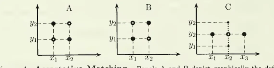
Figure 3:

Quasiconcavity.

The surplus functioninpanel

A

isnot quasiconcave, while those

in panels

B

and

C

are quasiconcave, but have flat portions that aren't globalmaxima. Neither is

stronglyquasiconcave. The surplus function in panel

D

is stronglybut not strictly quasiconcave.

That Al-Sup

or

Al-Sub

is a key ingredient ensuring a quasiconcave surplus function follows

from

the analysis of the frictionless

model

in section 2. For example,

under

Al-Sup,

the slope of x's frictionless surplus function,

_f

y(x,y)

—

f

y(y,y), is

positive iff

x

>

y.

We

illustrate the 'importance' ofour other

assumptions

(i.e. that

they are

sometimes

necessary conditions)

through two examples now,

and

one

later.

Example.

(Importance of

A2-Sup

or

A2-Sub)

The

production function

f(x,y)

=

(x

+

_y)2,

which

generated the

non

quasiconcave surplus functions in

Fig-ure 2, satisfies

Al-Sup, A2-Sub, and

both

A3-Sup and

A3-Sub.

Similarly, for the

production function f(x,y)

=

x

2

+

y2

+

x

+

y

—

xy

satisfying

Al-Sub, A2-Sup,

and

A3-Sup and

A3-Sub,

the surplus function is

sometimes

not quasiconcave.

Example.

(Importance of

A2-Sup*

or

A2-Sub*)

Consider the class of

pro-ductionfunctions f(x,y)

=

xy+c(x+y),

which

satisfy

Al-Sup, A2-Sup,

and A3-Sup,

but not

A2-Sup*.

Putting c

=

x(^/o~2

+

A8p

-

S)/A(r

+

5),

where

x

=

_J

Q zt(z)dz is

the

mean

populationtype, neatly yields

w(x)

=

ex in equilibrium; thus s(x, y)

=

xy

—

i.e. all

matches

are

weakly

agreeable.

But

type

x

=

produces

exactly zero surplus in all matches,

and

may

elect

an

arbitrary

nonconvex

matching

set.

Lemma

5 asserts: Ifthe

own-marginal product

of a given type is the

same

for a

sure

match

with z as for a

random match

from

some

set

M,

then

any

higher type has a lower

own-marginal product from

the

match

with z

than

with

M.

Lemma

5

(Single-Crossing

Property).

Posit AO.

Assume

Al-Sup and

A3-Sup

or

Al-Sub and

A3-Sub.

Choose any

y\

G

[0,1]

and

subset

M

C

[0,1]. Let

z solve

L

f

v(x,yi)u(x)

dx

, .

f

y(z,Vl)

=

Jm

7

7;;

^ (20) J

M

u(x)dx

Then

z is uniquely defined,

and

for all _y2

>

y\,

J

M

f

y(x,y2

)u(x)dx

f

y{z,y2)

<

I

M

u

(

x

)

dx

(21)

Remark

8.

One

can verify that (21) binds for production functions ofthe

form

f(x,y)

=

Ci

+

c2 (g(x)

+

g(y))

+

c3 h(x)h(y)

--

i.e.

where both

A3-Sup

and

A3-Sub

obtain, as

_f

xy(xi,y)/fxy (x2,y) is

independent

of y.

So

Lemma

5 is quite tight; in

fact, (21) is reversed if

Al-Sup

and

A3-Sub

(or

Al-Sub

and A3-Sup) both

obtain.

Next, for the formal proof of

Theorem

1,

we

give a convenient characterization

ofquasiconcave functions that are almost

everywhere

differentiable.

Q-l.

Ifo{y)

>

o{x)

and

o'(x) is defined, _{then y}

^

x

implies a'(x)

_^

0, Vx,y.

Q-2.

Ifcr(y)

>

a(x)

and

cr'(x) is defined, _{then y}

_^

x

implies a'(x)

_^

0, Vx,y.

Lemma

6.

A

continuous

and

almost everywhere differentiable

map

cr : _{[0, 1]} i

—

>-

M

is (a) strongly quasiconcave

under

Q-l,

and

(b) strictly so

under

Q-2.

If

a

is differentiable

on

(0,1), this

lemma

admits

a simple proof. Suppose, for

example, that

a

is not strictly quasiconcave but

Q-2

holds.

Then

there exists yi

<

2/2

<

2/3, with

a(y

2)

<

min(a(yi),a(y

3 )}. Since

a{y

]

)

>

a(y

2)

and

y1

<

y2, o'{y2)

<

by

Q-2. Similarly,

a(y

3)

>

a(y

2) implies a'(y2)

>

by

Q-2. This is a contradiction.

We

appendicize the general proof, for

which

a'(y2)

need

not

be

defined.

Proof

of

Theorem

1. For fixed z, the surplus function s(z,y) is continuous

by

A0

and

Lemma

2. Also, s

y(z,y) is defined for a.e. y, since

/

is differentiable

by

A0

and

w'(y) is defined for a.e. y

by

Lemma

3.

We

establish quasiconcavity using the characterization in

Lemma

6.

Namely,

we

prove thatforall z

and

_yx

<

y2,

(*)

holds:

if s

y(z,y\) exists

and

s(z,y2)

>

s(z,yr), then s_y(z,y±)

>

0,

under

supermodularity.17

•

Step

1:

Conclusion of

_(*)

is

Valid

For

'High'

Types.

We

show

that

surplus isstrictly increasing at _j/i for large

enough

z.

Choose

y\ with w'(yi) defined.

Define z as in

Lemma

5 with

M

=

M.(yi)

and

use differentiability

Lemma

3:

.,_

N JM(yi )fy(

x

>yi)

u

(

x

)

dx

pJ

M

(yi )fy(

x iy^ u

(

x

)

dx

l( v (on,

M'^=

J

M

,w|

„

M

dx

>

2 {r

+ S)+pSmm)

u [x)d

^

mM

(22)

So

<

f

y(z,

y^

-

w'(yi)

<

f

y(z,yx )

-

to'(j/i)

=

s_y(z,yx)

Vz

>

z,

by Al-Sup.

•

Step

2:

Implication (*)

is

Valid

For

'Low' Types.

Fix y2

>

_yx.

From

17_For

theproof_{of y}2

<

yi => s_y(z,yi)

<

0, oneinsteadshowsthat the premise s(z,y2)

>

s(z,yi)

fails for high types in step 1, while the implication is valid for low types in step 2. Proofs under

submodularity are totally analogous.

the implicit equation (10)

and

inequality (11)

w(y

2)

-

w(yi)

>

/9_/m(j /1)(/(

x

_'^)

-

f{x,yi))u(x)dx

2(r

+

_8)+pf

U{n)

u{x)dx

Divide

through

by

w'(yx)

and

its definition

from

Lemma

3:

w(y

2)

-

w(

_yi)

>

J

myi)

(f(x,y2)

-

_f(x,yi

))u(x)dx

>

f(z,y

2

)-f(z,

yi) w'{yi)

_J

_M{yi)

f

y(x,yi

)u(x)dx

fy(z,yi)

By

A2-Sup,

the final inequality is true iff z

<

z, appropriately defined. For

by

A2-Sup,

_f

_y(z,_y')/fy(z,yi) is increasingin z for y'

>

_ylt as is itsintegralover y'

_G

[yx,y2\.

For

some

such z,

suppose

s(z,y2)

>

s(z,2/i)

&

w(y

2)

-

w(y

1 )

<

f{z,y

2)

-

f{z,yi).

Then

s

y(z,yi)

=

f

y(z,yi)

—

w'(yi)

>

0.

Under

A2-Sup*,

the final inequality in (23)

is strict ifz

<

z, so s(z,_y2)

=

s(z, y{) implies s_y(z,y{)

>

as well.

Apply

Lemma

6.

•

Step

3:

Every

Type

is

Either

'High'

or

'Low'.

Here, the key ingredient

is

A3-Sup:

Integrate inequality (21) over y2

6

[2/1,2/2])

and

divide

through by

(20).

Put

M

=

M(yi)

in the

numerator

and denominator,

and

replace _y2

by

y2, to get

f{z,y

2

)-f(z,

yi)

<

J

myi)

{f(x,y2)

-

f(x,yi

))u{x)dx

fy&Vl)

!-

M

._{yi

)fy{.^y\)u{x)dx

So

z satisfies inequality (23); if z

<

z then z

<

z also.

So

for

any

(2/1,2/2), the z

associated with that pair is larger

than

the z associated with 2/1 alone.

Proof

ofProposition 3.

Under

the basic assumptions,

by

Theorem

1, each agent z

has a strongly quasiconcave surplus function. If s(z,y)

>

for

some

y,

Theorem

1

establishes that (i) the set ofagents y for

whom

s(z, y)

>

is

convex

and

(ii) there

are at

most

two

types

who

produce

exactly zero surplus with z.

Whether

z

matches

with

these

boundary

types does not affect the convexity of

M(z).

If s(z,y)

<

for all y,

w(z)

=

by

(10),

and

so z

=

from

Lemma

1.

Agent

could choose a

non-convex

matching

set if a positive

mass

of

matches

happen

to yield zero surplus; even that

cannot

happen

under A2-Sup*,

for then each agent has

a strictly quasiconcave surplus function. Finally, if

A1,A2,A3-Sub

obtain, s(0,y) is

increasing in y,

and

so is trivially strictly quasiconcave.

Example.

(Importance of

A3-Sup

or

A3-Sub)

Finding examples

ofproduction

functions associated

with

non-quasiconcave surplus functions

obeying

Al-Sub

and