Publisher’s version / Version de l'éditeur:
Energy Policy, 39, 10, pp. 6376-6389, 2011-09-01
READ THESE TERMS AND CONDITIONS CAREFULLY BEFORE USING THIS WEBSITE.
https://nrc-publications.canada.ca/eng/copyright
Vous avez des questions? Nous pouvons vous aider. Pour communiquer directement avec un auteur, consultez la
première page de la revue dans laquelle son article a été publié afin de trouver ses coordonnées. Si vous n’arrivez pas à les repérer, communiquez avec nous à PublicationsArchive-ArchivesPublications@nrc-cnrc.gc.ca.
Questions? Contact the NRC Publications Archive team at
PublicationsArchive-ArchivesPublications@nrc-cnrc.gc.ca. If you wish to email the authors directly, please see the first page of the publication for their contact information.
NRC Publications Archive
Archives des publications du CNRC
This publication could be one of several versions: author’s original, accepted manuscript or the publisher’s version. / La version de cette publication peut être l’une des suivantes : la version prépublication de l’auteur, la version acceptée du manuscrit ou la version de l’éditeur.
For the publisher’s version, please access the DOI link below./ Pour consulter la version de l’éditeur, utilisez le lien DOI ci-dessous.
https://doi.org/10.1016/j.enpol.2011.07.038
Access and use of this website and the material on it are subject to the Terms and Conditions set forth at
A comparison of four methods to evaluate the effect of a utility
residential air-conditioner load control program on peak electricity use
Newsham, G. R.; Birt, B.; Rowlands, I. H.
https://publications-cnrc.canada.ca/fra/droits
L’accès à ce site Web et l’utilisation de son contenu sont assujettis aux conditions présentées dans le site LISEZ CES CONDITIONS ATTENTIVEMENT AVANT D’UTILISER CE SITE WEB.
NRC Publications Record / Notice d'Archives des publications de CNRC:
https://nrc-publications.canada.ca/eng/view/object/?id=511800cb-19b6-4526-86ab-381ff017129c https://publications-cnrc.canada.ca/fra/voir/objet/?id=511800cb-19b6-4526-86ab-381ff017129cA c om pa rison of four m e t hods t o e va lua t e t he e ffe c t of a ut ilit y
re side nt ia l a ir-c ondit ione r loa d c ont rol progra m on pe a k e le c t ric it y
use
N R C C - 5 4 0 1 9
N e w s h a m , G . R . ; B i r t , B . ; R o w l a n d s , I . H .
O c t o b e r 2 0 1 1
A version of this document is published in / Une version de ce document se trouve dans:
Energy Policy,
39, (10), pp. 6376-6389, DOI:
10.1016/j.enpol.2011.07.038
http://www.nrc-cnrc.gc.ca/irc
The material in this document is covered by the provisions of the Copyright Act, by Canadian laws, policies, regulations and international agreements. Such provisions serve to identify the information source and, in specific instances, to prohibit reproduction of materials without written permission. For more information visit http://laws.justice.gc.ca/en/showtdm/cs/C-42
Les renseignements dans ce document sont protégés par la Loi sur le droit d'auteur, par les lois, les politiques et les règlements du Canada et des accords internationaux. Ces dispositions permettent d'identifier la source de l'information et, dans certains cas, d'interdire la copie de documents sans permission écrite. Pour obtenir de plus amples renseignements : http://lois.justice.gc.ca/fr/showtdm/cs/C-42
A Comparison of Four Methods to Evaluate the Effect of a Utility Residential
Air-conditioner Load Control Program on Peak Electricity Use
Guy R. Newsham* (corresponding author), Benjamin J. Birt* and lan H. Rowlands** National Research Council Canada- Institute for Research in Construction
Building M24, 1200 Montreal Road, Ottawa, Ontario, KlA OR6, Canada tel: (613) 993-9607; fax: (613) 954-3733
guy.newsham@nrc-cnrc.gc.ca
* National Research Council Canada ** University of Waterloo
Abstract
We analysed the peak load reductions due to a residential direct load control program for air-conditioners in one jurisdiction in southern Ontario in 2008. In this program, participant thermostats were increased by 2°C for four hours on five event days (when systemwide capacity was expected to be strained). We used hourly, whole-house data for 195 load control participant households and 268 non-participant households, and four different methods of analysis ranging from simple spreadsheet-based comparisons of average loads on event days, to complex time-series regression. Average peak load reductions were 0.2- 0.9 kW per household, or 10- 35%. However, there were large differences (up to a factor of four) between event days and across event hours, and in results for the same event day/hour with different analysis methods. There was also a wide range of load reductions between individual households. Policy makers would be
wise to consider multiple analysis methods when making decisions regarding which demand-side management programs to support, and how they might be incentivized . Further investigation of what type of households contribute most to aggregate load reductions would also help policy makers better target programs.
Keywords
Residential; Peak Demand; Direct Load Control; Ontario Canada
Acknowledgements
This work was funded by the Program of Energy Research and Development (PERD) administered by Natural Resources Canada (NRCan), and by the National Research Council Canada. The authors are grateful to Milton Hydro, this study would have been impossible without their extensive support.
Abbreviated Title
Four Methods to Evaluate the Effect of an Air-conditioner Load Control Program
Introduction
Many jurisdictions in North America experience a peak demand for electricity on hot summer afternoons, primarily due to rising air-conditioning load1. In such situations utilities must import additional capacity (often at a cost premiumL deploy peak capacity generators, or reduce demand. There might not be the capacity to build
1
Some cold climate regions are winter-peaking. Winter peaks tend to occur in early morning and in the evening, when heating-related loads are added to increased lighting loads and residential activity loads. The focus of this paper, however, is summer peaks.
additional generation, transmission, and distribution fast enough to accommodate projected demand growth, and thus the frequency of peak demand problems is
expected to grow [e.g Porter, 2009]. Indeed, in Ontario, Canada, the peak demand for electricity is growing faster than total electricity use [Rowlands, 2008].
As a result, there is growing interest in partly addressing this issue on the demand side [Piette et al., 2005; Rowlands, 2008], that is by eliminating some electricity use on peak, or shifting it to non-peak times. This strategy is commonly called "demand response". Methods to facilitate this are being explored in all building types, including residential buildings.
One set of measures involves Direct Load Control (DLC). In this case, utilities install equipment to allow them to modify the operation of appliances during peak periods. Typically such control is only invoked for a few hours on a relatively small number of "event" days (when systemwide capacity is expected to be strained). Air conditioning (AC) units are the most common residential appliance to be controlled. Newsham & Bowker [2010] reviewed the effect of several North American AC DLC pilot projects and commercial programs. These programs used a variety of technologies, protocols and evaluation methods, and reported sustained on-peak reductions of 0.3- 1.2 kW per AC unit.
The AC DLC program we used as the basis of this paper was the Peaksaver program in Ontario, Canada [OPA, 2008]. This is a voluntary, opt in program implemented by municipal utilities, and there is some freedom for individual utilities to determine how
best to meet the broad program goals. Households are offered incentives to
participate, including a free communicating thermostat through which utility signals are enacted. This program has been very successful, with a reported 136,000 households signed up across the province by 2009 [KEMA, 2010], with an estimated total load reduction of 64.5 MW.
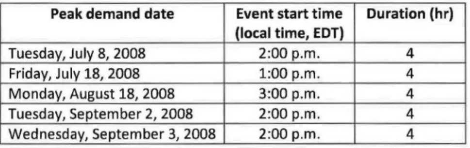
Table 1. The five Peaksaver events in summer 2008.
Peak demand date Event start time Duration (hr)
(local time, EDT)
Tuesday, July 8, 2008 2:00p.m. 4
Friday, July 18, 2008 1:00 p.m . 4
Monday, August 18, 2008 3:00p.m. 4
Tuesday, September 2, 2008 2:00p.m. 4
Wednesday, September 3, 2008 2:00p.m . 4
We used hourly, whole-house energy use data from 2008 from a municipal utility in southern Ontario. In this jurisdiction during the summer of 2008, there were five Peaksaver events (Table 1). In this case, an event involved the utility remotely
increasing the thermostat set point by 2°C for the duration of the event2. Participants could temporarily opt-out of the program, but were not notified of a Peaksaver event in advance3. We used these data to evaluate the DLC effect using four different
analysis methods. Woo & Herter [2006] reviewed and conceptually evaluated four
2
The most common current implementation of Peaksaver directly limits AC compressor run-time rather than resetting the thermostat.
3
When an event began the thermostat display indicated a DR mode, and participants could then enact a manual override.
different methods for evaluating the effect of residential demand response, with some overlap with the four methods evaluated in this paper. They noted the lack of an empirical evaluation of multiple methods on the same data set; the current paper fills this gap.
In the Methods section we first describe the dataset available for analysis, and then describe the four different methods used to estimate the on-peak reduction due to the Peaksaver program. The Results section presents the effect estimations for each method. The Discussion section suggests some explanations for differences in results by method, and makes some recommendations for the future use of methods by policy-makers. The main body of the paper focuses on effects for the mean load profile over all participating households, we also present results for individual households using one of the methods in Appendix A. Relating individual household load reductions to household characteristics suggests ways in which policy-makers may better-target load reduction programs. How programs are evaluated and marketed may have substantial effects on policy decisions.
Methods
A municipal utility in southern Ontario provided hourly data (from advanced, or "smart", meters) from 1297 residential accounts in 2008. 79% ofthese households were on a time-of-use tariff at the start of 2008 and the remaining households transitioned to time-of-use (from an increasing block rate) during April of 2008, thus the rate structure was the same for all households during the summer. 205 of the
sample households were enrolled in the Peaksaver program. 360 of the households provided data on household characteristics via a telephone survey in 2006 (as
described later, we used these households to construct a comparison group); only 7 of these households were also enrolled in Peaksaver.
We carried out a data cleansing process on the supplied data that removed households with excessive missing data and households with extreme values of energy use. If a house had a single hour of missing energy data in 2008, this hour was interpolated as the mean ofthe two hours on either side; if a house had more than a single hour of missing data in the year it was excluded from the analysis (37 were excluded from the initial sample of 1297). If a household's total, summer (May 1-0ct 31, as defined by utility tariffs), or winter (Jan 1-Apr30 and Nov 1- Dec 31) electricity use was more than three standard deviations from the mean value for that period, that household was excluded from the analysis as an outlier {30 were excluded from the remaining 1260). The number of households with both survey data and "cleansed" energy data was 327, and there were 195 Peaksaver households in the cleansed data set. Table 2 shows summary energy use information for the households in these samples4. On average, the energy use by the survey group and the Peaksaver group was very similar to that in the larger sample.
4
We had household characteristics data for the survey sample only, but we believe them to representative of the utility's residential accounts. Around 2/3 were single detached houses, with the remainder semi-detached or row houses; mean age 16 years; mean size 189 m2•
Table 2. Descriptive statistics for energy-related metrics, for 2008.
Larger sample (N=1230) Min. Max. Mean S.D. Total electrical energy used, kWh 613 19009 8481 3048 Total electrical energy used in Summer, kWh 187 10574 4499 1788 Total electrical energy used in Winter, kWh 426 9487 3982 1413
With survey data (N=327) Total electrical energy used, kWh 1957 18165 8722 3426 Total electrical energy used in Summer, kWh 627 10344 4575 2014 Total electrical energy used in Winter, kWh 1185 9451 4147 1606 Peaksaver participants (N=195) Total electrical energy used, kWh 614 19009 8694 2794 Total electrical energy used in Summer, kWh 187 10574 4606 1609 Total electrical energy used in Winter, kWh 427 8438 4089 1300
All weather data used for our analyses came from an Environment Canada station approximately 30km away [Environment Canada, 2010], the closest station with comprehensive hourly data .
We used four methods drawn from the literature to determine the mean load reduction during a demand response event. The first method compared the mean hourly energy use on an event day for households enrolled in the Peaksaver program to a control (i.e. non-participant) group [Rocky Mountain Institute, 2006]. The
remaining three methods did not utilize a control group. The second method, which is the more common non-regression method [Kempton et al., 1992; Cook, 1994; Herter et al., 2007; Navigant, 2008; Lopes & Agnew, 2010], compares mean hourly electrical energy use for Peaksaver houses on event days to use by those same houses on otherwise equivalent non-event days. The third method was a common multiple
regression technique [Summit Blue, 2004; KEMA, 2006; BGE, 2007; George & Bode, 2008; Ericson, 2009] in which events are independent variables in the regression equation for household electrical energy consumption, and the regression coefficients for the events are the estimates of the program effects. This third method, though relatively straightforward, ignores the explicit time-series nature of the data. The fourth method we used was a time-series regression, which is rarely employed with this kind of data, but which is common in economics [Montgomery et al., 2008]. All methods are described in more detail below.
Method 1: Comparison of Peaksaver group to a control group
It was desirable that the control group was equivalent to the Peaksaver group in
energy use in all ways other than being a Peaksaver participant. Peaksaver households all had central AC (a requirement for enrolment), whereas not all households in the larger data sample had AC. Therefore, we chose the control group from the smaller sample of surveyed households not in the Peaksaver program that indicated they had central AC. It was possible that some surveyed households had acquired, or disposed of, AC since 2006. Therefore we investigated the energy use of the surveyed
households with respect to external temperature. Seventeen households were added to the control group who said they had no air conditioner in 2006, but for which energy use data on hot afternoons suggested AC use5. Nineteen households were removed
5
from the control group that did not appear to use AC at all in 2008 but said they had one in 2006. The final control group contained 268 households.
It was still possible that there was a systematic difference in energy use behaviours between the Peaksaver and control groups that would bias effect estimates. Therefore, as an option, we further "matched" the two groups prior to Peaksaver events using a normalization factor, which was a multiplier applied to all hourly energy use values of the Peaksaver group on the event day. Several epochs for determining a normalization factor were tested, and we used a root-mean-square n RMS test to determine which one performed best. Epochs reviewed were various time periods on the same day of week, the week before, day before, day after, days with similar temperatures as the peak demand days, and the morning of the peak demand day. Overall, we found that the best epoch to use was from 9:01a.m. to noon on the day of the event. The normalization factor was the ratio of energy use by the control group to that of the Peaksaver group during this period. This was similar to an approach taken in commercial buildings [Piette et al., 2005L and has the benefit that it can be
performed when non-event days are not available.
Once the two groups were matched, the load reduction for a given event day and hour was obtained by simple subtraction:
With the concomitant percentage effect:
Ec -EP
Percentage reduction= ect,hc ect,h .100 Eed,h
(2)
Where ed and hare event day and hour indices, and セ・、LィL@ EPed,h is the hourly energy
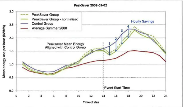
use on each event day for the control group and Peaksaver group, respectively. The process is shown graphically in Figure 1 for a single example event day; note that Figure 1 also shows how much higher electricity use on an event day was compared to an average, non-event, non-holiday, summer weekday (May 1st to October 31st, as defined by the utility company's time-of-use tariff schedule).
3.0
:E
.s::::. 2.5 セ@...
2.0 :::1 0 .s::::....
G) a. 1.5 G) II) :::1 :>. El G) 1.0 1:: G) 1:: lB :::1: 0.5 0.0 0 PeakSaver 2008-09-0Z PeakSaver Groupr
PeakSaver Group - normalised
Control Group 1 - - - : - -H_o_urly Savings
Average Summer 2006
Peaksaver Mean Energy
Aligned with Control Group
'
- - -- -- -MMセセ MMMMMMMM⦅ LNNN@ _ _ J ___ __ _ ___ _ - - - ---- -
-'
I I
: Event Start Time
I
-T - - - , --- ----,.--- - --r-- ---- -,- - - - ---r ---.- r-
r-2 4 8 10 12 14 16 18 20 Time of day
22 24
Figure 1. Determination of the mean hourly savings made by houses enrolled in the Peaksaver program. The mean Peaksaver profile (dashed green line) is normalized (solid green line) to match the control group (purple line) during pre-event periods. Subtraction of the two profiles gives the hourly electrical energy savings from the start of the Peaksaver event.
Method 2: Comparison of Peaksaver group on event days to non-event days
Previous studies have defined an equivalent non-event day as one with a similar temperature profile, defined in various ways (e.g. Kempton et al., 1992;
Egan-Annechino et al., 2005; Lopes & Agnew, 2010]. In this analysis we sought equivalent days (non-holiday weekdays) by first comparing average daily temperature and retaining possible matches ifthey were within 5%; we also compared the maximum and minimum temperatures and the number of hours above 24°C in the day. We then plotted the remaining daily profiles and selected the closest match by visual inspection . Preference was given, where possible, to days that were closest in the calendar to the event day to control for seasonal effects or household behaviour patterns.
Temperature data for event days and their resulting equivalent day are shown in Table 3.
Table 3. Temperature data for event days and their resulting equivalent day.
Event date Temperature (
0
C} Hours Equivalent Temperature (0
C} Hours
Mean Min. Max. above 24°C date Mean Min. Max. above 24°C
July gth 25.4 20.3 30.7 11 June gth 25.1 19.4 33.1 14
July 18th 25.5 22.4 28.6 17 July 16th 24.7 19.2 30.9 15
August 18th 23.0 18.2 29.4 11 August 6th 22.7 18.1 27.4 9
September 2"d 21.5 15.2 26.1 9 July 29th 21.7 16.1 26.2 8
September 3rd 23 .3 16.0 30.3 10 July 1ih 25.6 21.2 30 17
As in Method 1, we again explored a normalization process to account for residual variation in energy use between the event and equivalent days. Normalization was performed using a similar procedure as in Method 1, and again the normalization
factor was based on the mean energy use from 9:01 a.m. to noon on the day of the event, the factor being the ratio of energy use by the Peaksaver group on the event day to that on the equivalent day, and applied to the equivalent day. Again, the load reduction for a given event day and hour was obtained by simple subtraction:
Load reductioned,h
=
eAセィ@
-
eセ、Lィ@
With the concomitant percentage effect:
EEQ EP
Percentage reduction= ed,hE-Q ed,h .100 Eed,h
(3)
(4)
Where EEaed,h is the hourly energy use on each event day for the Peaksaver group on
the equivalent non-event day.
Method 3: Simple, multiple regression
A simple, multiple regression uses a least squares estimation approach to solve an equation ofthe form:
(5)
Where
Yt
is the hourly electricity use at hourt,
Xi is a series of independent predictorvariables,
ft
are the regression coefficients associated with these predictors, and Et is arandom error. A large number of statistical software packages exist to solve this equation; we used the SPSS v.18 REGRESSION procedure. When the predictor variables represent event hours, their regression coefficients are the estimate of the effect of the event.
There is a considerable art in selecting the predictor variables so that effects not
directly related to the event are appropriately accounted for, such that the event effect estimates are reasonable. The choice of these variables differs in the literature. We based our choices on an amalgam of those that were successful in prior studies and some trial-and-error assessment of the face validity of results. Some authors have chosen to develop separate equations for each hour of the day [e.g. Hartway et al., 1999; BGE, 2007], and others have chosen a single equation with dummy variables for each hour [e.g. George & Bode, 2008; Herter & Wayland, 2010]; we chose the latter approach. Our final model specification was:
Yt
= "LT=oPcvH24,lCDH24t-l
+"LT=o fJRH,lRHt-l
+PNwvNWDt
+PsrSTt
+lセ]VヲjmthLュmthュLエ@
+lセ[ャーhrLィhrィLエ@
+lセ[ャーeャLィeQィLエ@
+lセ[ャーeRLィeRィLエ@
+lセ[ャ@
PE3,hE3h,t
+lセ[ャ@
PE4,hE4h,t
+RNセ[Q@
PEs,hESh,t
+Et
(6)
where,
CDH24t-t is the cooling degree hours, base 24°C (i.e. outside air temperature minus 24), at time
t
andI
hours prior to timet,
these lag terms account for heat stored in the building fabric, base 24°C was chosen to be compatible with Herter & Wayland [2010] who successfully used 75°F as a base for a California study;RHt-t is the relative humidity (%) at time
t
and I hours prior to timet;
NWDt is a dummy variable to indicate if the current hour tis within a normal weekday (i.e. Monday- Friday, non-holiday);
STt is a dummy variable to indicate ifthe current hour tis within the school term, this may vary between schools, but was standardized here as up to and including June 26th and after and including September 2nd;
MTHm,t is a dummy variable to indicate ifthe current hour tis within month m, regressions are run for summer months only (May- October) and effects are referenced to month 5 (May) as the summer month with the lowest average use;
HRh,t is a dummy variable to indicate ifthe current hour tis within hour h, effects are referenced to hour 5 (4:01- 5:00a.m.) as the hour with the lowest average use;
ElM is a dummy variable to indicate if the current hour tis within hour h of the first event day; E2 ... E5 reference the other event days similarly.
The method is easily expanded to add further dummy variables for individual hours on the day before and after events to explore energy use modifications pre-event and "snapback" (or "rebound") behaviour extended in time [Herter & Wayland, 2010], we did this, but for brevity do not report the results here. It is also straightforward to solve an equation for each household separately. This can be useful in exploring the range of contribution to the load reduction across households, we report on this in Appendix A.
Method 4: Time-series regression
Although conceptually straightforward, the simple regression explicitly ignores the time-series nature of the data. That is, despite all of the other climatic and temporal influences on electricity use at 3 p.m. on a given day (for example), it also follows from
electricity use at 2 p.m., and uses at 2 p.m. may influence uses at 3 p.m. For example, laundry that began at 2 p.m. may still be active at 3 p.m. Further, the habitual use of electricity may mean that electricity use at 3 p.m. on one day is similar to use at 3 p.m. the previous day, or on the same day the previous week. Accounting for the "within subjects" nature of the data is conceptually more correct, and should improve estimates of effects [Woo & Herter, 2006). Some of the time-series effects may be represented by dummy variables (for hour, for example) in the simple regression equation. One could also add lag terms for the outcome variable as predictors (adding
f3Yt-l
etc. to the right-hand side of Eq. (6), e.g. Henley & Peirson, [1998)) similar to theuse of lag terms in climatic variables. A more complex, but more comprehensive, class of models to deal with such time-series data is named ARIMAX (Auto Regressive
Integrated Moving Average with eXternal (or eXogenous) input) and was developed for forecasting in other domains, particularly in economics [Montgomery et al., 2008). The "integrated" part of the name indicates that the analysis is often run on the change in the dependent variable of interest (known as "differencing"), to render the series stationarl. "Auto regressive" (AR) indicates that the forecasted value of the dependent variable may be predicted from prior, known, values of the dependent variable. "Moving average" (MA) indicates that the forecast may be predicted from prior values of the error term. "External input" refers to the optional use of
independent predictors. Often the variable of interest exhibits periodic behaviour,
6
In a "stationary" series the values vary around an unchanging mean, and the variance over time is constant. Stationary series are a requirement for ARIMA models.
generally referred to as "seasonal" behaviour. For example, building energy use often displays a diurnal pattern; if one measures energy hourly then there will be a
seasonality of order 24. For modelling, one creates a new seasonal variable to reflect this variation, which is the current value ofthe dependent variable minus the value from one seasonal period ago. One can then apply differencing and lags to this variable and include these terms in the model.
The most general mathematical form of the ARIMAX model equation is as follows [SAS, 2011]:
(7)
where,
t
indexes time, ands
is the order (length( of the seasonal cycleYt
is the dependent time seriesX,t
is a set of i external predictor time seriesat
is a white noise time series representing random errord, D is the number of times the dependent variable (and seasonal dependent variable) are differenced
11
is the mean of the series (=0 when series is differenced)B
is the backshift operator; i.e.BYt= Yt-1: B12Yt= Yt-12; BB12Yt= B
13Yt
c/Js{f3s)
is, similarly, the seasonal autoregressive operator, a polynomial of orderP:
B(B)
is the moving average operator, a polynomial of orderq
in the backshiftoperator:
Bs{f3s)
is, similarly, the seasonal moving average operator, a polynomial of order Q :セサbI@ is a transfer function for the effect of
X;ton
Yt:
r5i(B) is the denominator polynomial in the backshift operator, for the ith predictor:
8·(8)
t=
1-8·18-· .. -8 . .
t, t,pt BPirSM(B)
is similarly, the denominator seasonal polynomial, for the ith predictor:8
S,t·(B)=l-8 ·18- ..
S,l,·-/S
S,t·p.BsPi1 t
u)j{B)
is the numerator polynomial in the backshift operator, for the ith predictor:W·(B)
t =W·
t, 0 -w-
t, 18 -
... - W· .Bqi
t,qtWs,i(B)is similarly, the numerator seasonal polynomial, for the ith predictor:
W ·(B)=w ·
S,l S,l, 0-w ·
S,l, 18 - ..
·-w ·Q.B
S,l., t 5Qi
.k
·is the time delay for the effect of the ith predictor (if the predictor cannot affect the dependent variable for a certain number oftime steps for basic physical reasons)ARIMAX models have been used in building-related applications, including modelling of water and fuel use [Lowry et al., 2007], and forecasting and controlling the peak
demand for electricity [Hoffman, 1998]. Herter & Wayland [2010] used a limited form of this method, with auto-regressive lag 1 terms only, in an analysis ofthe effect of pricing regimes on peak household electricity use.
We used the SPSS v.18 TSMODEL routines, with climate variables, dummy variables for normal weekday and school term, and dummy variables for Peaksaver event hours. Note that SPSS automatically determines the best fitting models and lag terms. This will serve for our immediate purpose but is somewhat limiting, and there are other statistical packages that offer more options.
Results
Method 1: Comparison of Peaksaver group to a control group
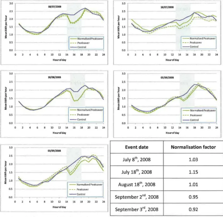
Figure 2 shows the mean daily electrical energy use profiles for the control group (purple line), normalized Peaksaver group (green line), and unnormalized Peaksaver group (dashed green line) for each event day. The electrical energy use profiles ofthe control group and the normalized Peaksaver group generally match each other pre-event, except for July 18th. The pre-dawn energy use on July 181h is the same for both
groups before normalization. However due to the Peaksaver group using less energy between 9:01 a.m. and noon (normalization factor greater than 1) the norm.alized curve is above the control group curve in the pre-dawn hours. Due to the relatively large normalization factor the relative savings are potentially underestimated for this
day. The temperature on August 18th dipped dramatically between 1 p.m. and 2 p.m., most likely due to storm cells passing through the region, and is reflected by a dip in the energy use in both groups.
Studies in the literature have frequently (but not universally) observed an increase in electricity use by DLC participants after an event. This may be explained by AC units working hard to restore thermostat setpoints, and other electricity uses postponed during event hours. This phenomenon is sometimes referred to as "snapback" or "payback". One might also observe higher use pre-event due to manual pre-cooling or other use of electricity in anticipation of the event. There was no consistent evidence of such behaviour by the Peaksaver group, but note that comparison of energy use pre-event will be masked by the normalization process.
3.0 2.5 セ@ _g 2.0 セ@ 0. セ@ 1.5 セ@ :ii Gl 1.0 ::; 08/07/2008 0.5 MMM M M セ MMM M 0.0 10 12 14 16 18 20 22 24 Hour of day 3.0 2.5 セ@ セ@ 2.0 0 ..c
..
0. ..c 1.5 セ@ セ@ 1.0 セ@ セ@ 0 ..c セ@ 0. ..c セ@ lij セ@ セ@ 0 ..c セ@ 0. ..c セ@ iii セ@- - -
-3.0 lB/07/2008 2.5 2.0 1.5 1.0 - - Normalised Peaksaver 0.5 - - - Peaksaver - - control 0.0 4 10 12 14 16 18 20 22 Hour of day- - -
-3.0 02/09/2008 2.5 2.0 1.5 1.0::; - Normalised Pea ksAvet ::;
- - Normalised Pcak.s.aver セ@ 0 ..c セ@ 0. ..c セ@ iii セ@ ::; 0.5 - - - Peaksaver - - control 0.0 0.5 r -0.0 -- - - - Peaksaver - - Control 0 4 10 12 14 16 18 20 22 24 4 10 12 14 16 18 20 22 24 Hourofday Hour of day
3,0 Event date Normalisation factor
113/09/2008 2.5 July 8th, 2008 1.03 2.0 1.5 July 18th, 2008 1.15 1.0
- Normalised Peaksaver August 18th, 2008 1.01
0.5 - - - Peaksaver - - control 0.0 September 2nd, 2008 0.95 0 4 10 12 14 16 18 20 22 24 Hour of day September 3'd, 2008 0.92
Figure 2. The mean daily electrical energy use profiles for the five peak demand days for the two groups (Peaksaver and control).
Table 4 lists hourly load reductions for each of the four event hours on each event day, and the mean for the event as a whole; calculations for the normalized and
unnormalized Peaksaver group are shown. Load reductions generally decrease over the course of the event, which might be due to participants opting out as conditions decline, or to AC restarting as the higher setpoint is reached. Load reductions for individual event hours (normalized) ranged between 0.21 kWh/h and 0.58 kWh/h or 9.6% and 30.1%.
Table 4. Mean hourly savings per house in the study group from the start of the event.
Comparison Hour1 Hour2 Hour3 Hour4 Event mean
Event date kWh/h % kWh/h % kWh/h % kWh/h % kWh/h % Unnormalized 0.53 23 .6 0.56 24.7 0.55 22.6 0.48 18.4 0.53 22.2 JulyS, 2008 Normalized 0.47 21.0 0.50 22.1 0.49 20.0 0.41 15.7 0.47 19.6 July 18, Unnormalized 0.54 28.4 0.47 23.7 0.56 26.3 0.47 21.2 0.51 24.8 2008 Normalized 0.34 17.8 0.25 12.4 0.33 15.4 0.21 9.6 0.28 13.7 August 18, Unnormalized 0.56 29.6 0.54 28.2 0.52 24.2 0.33 14.2 0.49 23.6 2008 Normalized 0.55 28.7 0.52 27.5 0.50 23.3 0.30 13.2 0.47 22.7 September Unnormalized 0.27 15.9 0.27 14.8 0.29 13.3 0.22 9.3 0.26 13.0 2,2008 Normalized 0.35 20.5 0.36 19.4 0.39 18.1 0.33 14.2 0.36 17.8 September Unnormalized 0.46 23.6 0.40 19.3 0.22 9.7 0.09 3.6 0.29 13.3 3, 2008 Normalized 0.58 30 .1 0.55 26.1 0.39 17.3 0.29 11.8 0.45 20.7 Unnormalized 0.47 24.2 0.45 22.1 0.43 19.2 0.32 13.4 Hour mean Normalized 0.46 23.6 0.43 21.5 0.42 18.8 0.31 12.9
Method 2: Comparison of Peaksaver group on event days to non-event days
Figure 3 shows the mean energy use profile for the Peaksaver group on event days and for the same group on equivalent non-event days. In all five graphs, the event day is the green line and the normalized equivalent day is the purple line. The unnormalized equivalent day has a different colour in each graph as each event day has a unique equivalent day. Where possible the day before (solid grey line) and the day after (dashed grey line) were also plotted for comparison. If a grey line is missing it means
that the day before/after was a weekend, public holiday, used as the equivalent day, or was an event day itself.
:;: 3.0 , :;: 2. 5
r-セ@ i 2. 0 セ@i
1.5 t: " > "§ 1.0 . 0 .J: セ@ "0.5 l -::;: PNP ᄋMMセセ@ 2.5 0.0 3.5 セ@ 3.0 .J:!
2.5 セ@ セ@ 2.0 " 5i 1.5 > 1i _g 1.0 セ@ セ@ 0.5 0.0 0 0 4 08/07/08 - - Eventday - Equivalent Day- Nor·m· a. lis.ed Equivale nt Day セ@ 1 DayBefore セ@ _ ャ_セケ。ヲエ・イ@ 10 12 14 16 18 20 22 24 Hourofday 18/08/08 l - EventDay - -1 - Equivalent Day
j - Normalised Equivalent Day
; DayAfter 10 12 14 16 18 20 22 24 Hour of day 03/09/08
!
-Event Dayr
- Equivalent Day - - Normalised Equivalent DayDay After 10 12 14 16 18 20 22 24 Hour of day 3.5 セ@ 3.0 f - - - 18/07/08 ..1: 3: :!. 2.5 Q MMMMMセMM :i: セ@ 2.0 セ@ ; 1.5 > "1: _g 1.0 セ@ セ@ 0.5 0.0 4 3.0 . .
--1
- EventDay - Equivalent Day- Normailsed Equivalent Day
10 12 14 16 18 20 22 24 Hourofday 02/09/08 .J: :;: 2.5 f -セ@
i
2.0 セ@ セ@ 1.5 t: " > セ@ 1.0 セ@ セ@ G.l 0.5 ::;: 0.0 4 Event date July 8, 2008 July 18, 2008 August 18, 2008 September 2, 2008 September 3, 2008I
- EventDay - Equivalent Day - Normalised Equivalent Day 10 12 14 16 18 20 22 24 Hour of day Normalization factor 1.09 0.82 0.97 0.99 0.89 Figure 3. Mean daily energy use profiles of the Peaksaver enrolled households. Event days are green lines; normalized equivalent days are purple lines; unnormalized equivalent days have a different colour in each event day graph; and the days before and days after are grey and dashed grey lines respectively.There was a large variation in the energy use profiles across supposedly similar days, and thus finding an equivalent day was difficult (Table 3). Only for the first and last
event days (July
ih
and September 3rd) was there a good match between the event and equivalent days for non-event hours. Similar to Method 1, for the event on July 18th there appears to be a reduction in energy use in the hours leading up to the event. This reduced energy use affects the normalization factor and makes it difficult to get an energy use profile from an equivalent day to match this day.Table 5 shows the hourly load reductions on event days and the mean reduction for each event; calculations for normalized and unnormalized equivalent days are shown. Here, load reductions tend to rise early in the event, before decreasing in later event hours. Load reductions for individual event hours (normalized) ranged between 0.09 kWh/h and 0.83 kWh/h, or 4.0% and 32.8%.
Table 5. Mean hourly savings per house in the study group from the start of the event.
Event Date Comparison Hourl Hour2 Hour3 Hour4 Event mean
kWh/h % kWh/h % kWh/h % kWh/h % kWh/h % Unnormalized 0.35 16.8 0.62 26.6 0.42 18.1 0.29 12.1 0.42 18.4 July 8, 2008 Normalized 0.54 23.8 0.83 32.8 0.63 25.0 0.51 19.5 0.63 25.3 July 18, Unnormalized 0.83 38.1 0.77 33.7 0.79 33.6 0.93 34.8 0.83 35.0 2008 Normalized 0.43 24.3 0.35 18.9 0.36 18.8 0.44 20.3 0.40 20.5 August 18, Unnormalized 0.39 22.3 0.57 29.5 0.56 25.6 0.25 11.2 0.44 21.9 2008 Normalized 0.34 20.0 0.52 27.4 0.50 23.4 0.18 8.5 0.38 19.6 September Unnormalized 0.23 14.0 0.27 14.8 0.17 8.5 0.12 5.2 0.20 10.2 2,2008 Normalized 0.21 12.9 0.25 13.7 0.15 7.3 0.09 4.0 0.17 9.1 September Unnormalized 0.69 39.4 0.58 33.6 0.50 28 .4 0.49 26.2 0.57 23.0 3,2008 Normalized 0.46 23.8 0.33 16.4 0.23 9.9 0.18 7.1 0.30 13.6 Unnormalized 0.50 26 .1 0.56 27.6 0.49 22 .8 0.42 17.9 Hour mean Normalized 0.40 20.9 0.46 21.8 0.37 16.9 0.28 11.9
(Constant) セ cdhRTLP@ セcdhRTLQ@ セcdhRTLR@ セcdhRTLS@ セcdhRTLT@ セ cd h RTLU@ セcdhRT@ 6 f3 RH,O セrhLャ@ f3RH,2 f3 RH,3 f3RH,4 セrhLs@ セrhV@ f3NWD f3sr f3M TH,S f3MTH,6 f3MTH,7 セmth LX@ セmthLY@ f3MTH,10
Method 3: Simple, multiple regression
Table 6 shows the regression coefficients resulting from the use of Eq. (6) on the mean energy use for the Peaksaver households; hourly data encompassing the entire six summer months (May- October) was used. The coefficients represent effects in kWh/h .
Table 6. Regression coefficients (B) for solution of Eq. (6} on summer 2008 data. Statistically significant coefficients H。セoNosI@ are shown in bold; coefficients associated with Peaksaver event hours are shaded.
B B 0.457 セhrLャ@ 0.270 セeャ L ャ@ 0.097 セhr LR@ 0.137 セeャ LR@ 0.026 セhr LS@ 0.067 セeQLS@ 0.034 セhrLT@ 0.021 セeャLT@ 0.016 セhrLs@ REF セeャLs@ 0.010 セhrLV@ 0.024 セeャLV@ 0.003 セhrLW@ 0.128 セeQLW@ 0.113 f3HR,8 0.248 セeャ Lb@ 0.000 f3HR,9 0.305 セeQLY@ 0.000 f3HR,10 0.354 f3et ,lo 0.000 f3HR,ll 0.400 セeャ Lャャ@ 0.000 セhr LャR@ 0.421 セeャLャR@ 0.000 f3HR,l3 0.445 セeャLQS@ 0.002 セhrLQT@ 0.427 セeQLQT@ -0.001 セhrLャs@ 0.422 f3El,l5 -0.194 セhrLャV@ 0.444 f3El,l6 -0.282 セhrLャW@ 0.543 f3et,17 REF f3HR,l8 0.677 13El,l8 0.476 f3HR,19 0.751 セeQ LQY@ 0.436 f3HR,20 0.737 f3El,20 0.311 セhr LRQ@ 0.731 f3et,21 0.426 f3HR,22 0.739 f3E1,22 0.070 f3HR, 23 0.652 f3El,23 f3HR,24 0.465 f3et,24 2 F164,441s=122.2, R adj=0.818 B 0.026 0.09 2 0.063 0.153 0.240 0.234 0.222 0.130 0.022 0.033 0.001 -0.155 -0.023 -0.116 -0.840 -0.929 -0.933 -0.864 0.085 0.189 0.250 0.356 0.357 0.279 8 8 8 セeR L Q@ -0.023 セeS L Q@ 0 .306 セeT L Q@ 0.350 f3Es ,l セeR LR@ 0.133 f3E3,2 0.303 セeT L R@ 0.277 セeU L R@ セeR LS@ 0.132 セeSLS@ 0.237 セeT L S@ 0.222 f3Es,3 セeRLT@ 0.163 セeSLT@ 0.200 セeT L T@ 0.233 セeU L T@ セeRLU@ 0.207 セeSLU@ 0.177 セeT LU@ 0.182 セes L s@ セeR LV@ 0.214 セeSLV@ 0.175 セeT L V@ 0.182 セes L V@ セeRLW@ 0.220 セeSLW@ 0.143 セeT LW@ 0.202 セeU L W@
f3ez ,s 0.179 f3e3,s 0.105 セeT L X@ 0.210 f3es ,a
セeR L Y@ 0.078 f3e3,9 0.287 セeT L Y@ 0.266 f3es,9
セeR LQP@ 0.011 f3e3,10 0.290 f3e4,1D 0.130 f3es, to
セeR L ャャ@ -0.057 f3E3 ,11 0.163 セeT L QQ@ 0.382 f3ES,ll
セeR LQR@ -0.147 セeSLQR@ 0.082 セeT L QR@ 0.448 f3es ,t2
セeRLQS@ -0.270 セeSLQS@ 0.051 セeTLQS@ 0.385 f3es.l3
f3e2.14 -0.604 セeSLQT@ 0.064 f3e4,14 0.416 f3es,l4 f3e2,1S -0.570 セeSLQU@ 0.258 f3e4,ls 0.242 f3ES,l5 f3e2.16 -0.642 13e3,16 -0.361 13e4,16 0.182 f3es,l6 f3e2,17 -0.602 f3e3,17 -0.558 f3e4,17 0.420 13es,t7 f3e2 ,1B -0.389 f3e3,1B -0.443 f3e4,1B 0.577 f3es,ts f3e 2,19 -0.425 f3e3,19 -0.141 f3e4,19 0.860 f3es,t9 f3e2,2D -0.401 セeSLRP@ 0.028 セe TLRP@ 0.770 セeULRP@ f3e2,21 -0.376 セeS LR Q@ 0.409 f3E4,21 0.750 f3ES,21 f3e2,22 -0.453 f3e3,22 0.448 f3e4 ,22 0.679 f3ES,22
セeRLRS@ -0.034 f3E3,23 0.360 f3e4,23 0.486 f3es,23
f3e2,24 0.182 f3e3,24 0.267 f3e4,24 0.442 f3es,24
Overall, the simple regression performed well, with the predictor variables explaining more than 80% of the variance in electrical energy use. As expected, coolingdegree
-8 0 .517 0.393 0.333 0.254 0.241 0.257 0.293 0.308 0.294 0.235 0.204 0 .211 0.147 0.120 -0.461 -0.518 -0.337 -0.106 0.063 0.134 0.523 0.509 0.378 0.344
hour coefficients were positive, suggesting higher temperatures in summer led to high electricity use; both cooling-degree-hours in the hour under consideration, and some lag terms, were statistically significant. Only one lag term in relative humidity was significant, and the coefficient was positive, as expected. The normal weekday term was statistically significant and negative; as commonly observed, households tend to use more electricity on weekends and holidays than on weekdays, when people are at home for more hours, on average, and some energy-intensive uses are conducted (e.g. laundry). Similarly, the school term coefficient was significant and negative; less energy was used on days when children are at school rather than at home. The month coefficients were positive and significant, relative to May; the June coefficient was higher than all others, but that most days in June are also school days, which adjusts overall usage down. The set of hourly coefficients describes the average hourly profile, with energy use at a minimum in the early morning, and at its highest mid-evening.
The effects of the Peaksaver events are shown by the five pairs of columns at the right of Table 6, in which statistically significant load reductions during the event are
indicated by negative coefficients in bold text in shaded cells. For the first two events there were statistically significant reductions for all four hours of the event. For the third and fifth events all event hours presented negative coefficients, but only two of four hours were statistically significant. The fourth event was unusual in that the regression results suggest electricity use was actually higher than normal during the event. In fact, energy use was higher for all hours of this day, suggesting something occurring on this day that was not captured by the variables in the equation. One
possibility is that this coincided with the start of the school year, a one-day effect distinct from the multi-week school term predictor7. By looking at the hours
immediately after the conclusion of the Peaksaver event, there was no consistent evidence for snapback. The third and fifth events showed statistically significant increased usage in the evening hours following the event hours, but the second event suggested continued lower usage in these hours. Neither do the results suggest substantial pre-event effects.
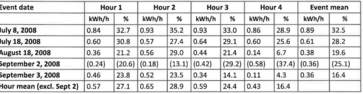
Percentage effects were determined from the coefficients in Table 6 and the predicted usage absent the Peaksaver event. These are summarized in Table 7 for comparison with the earlier methods. Ignoring the fourth event, individual hourly load reductions ranged from 0.11-0.93 kWh/h per household, or 4.3-35.2 %.
Table 7. Mean hourly load reduction per house in the Peaksaver event from the start
of the event, based on the simple regression results .
Event date Hour1 Hour2 Hour3 Hour4 Event mean
kWh/h % kWh/h % kWh/h % kWh/h % kWh/h % JulyS, 2008 0.84 32.7 0.93 35.2 0.93 33.0 0.86 28.9 0.89 32.5 July 18, 2008 0.60 30.8 0.57 27.4 0.64 29.1 0.60 25.6 0.61 28.2 August 18, 2008 0.36 21.2 0.56 29.0 0.44 21.4 0.14 6.7 0.38 19.6 September 2, 2008 (0.24) (20.6) (0.18) (13 .1) (0.42) {29.2) (0.58) (37.4) (0.36) (25.1) September 3, 2008 0.46 23.8 0.52 23.5 0.34 14.1 0.11 4.3 0.36 16.4 Hour mean (excl. Sept 2) 0.57 27.1 0.65 28.9 0.59 24.4 0.43 16.4
7
One way to account for this kind of effect is to include a variable that represents individual days. For example, we ran a regression with the use at 10 a.m. on each day as a predictor variable, essentially raising or lowering the overall daily profile depending on whether it starts out as an unusually high or low use day, this improved the model fit, but for brevity we do not report the results here.
We applied the same regression equation to the data from each household separately. The results are detailed in Appendix A, and show (depending on how conservative the method of analysis) that as few as 12% or as many as 83% of Peaksaver participants contributed load reductions for a given event hour.
Method 4: Time-series regression
Table 8 shows the model parameters resulting from the use of Eq. (7) on the mean energy use for the Peaksaver households; hourly data encompassing the entire six summer months {May- October) was used. The parameters are not as straightforward to interpret as for the simple regression, but for our purpose the parameters labelled "numerator" represent effects of the predictor variables in natural-log(kWh/h). Note, SPSS v.18 TSMODEL output only shows statistically significant effects. The upper part of the table shows the lag terms in the outcome variable used as predictors. This is followed by the climate variables, note that cooling-degree-hours was a significant predictor but humidity does not add predictive power; recall humidity's role in the simple regression was very minor. Normal weekday was a significant, negative
predictor, as in the simple regression, but the dummy variable for school term did not add predictive power here. The event-hour terms, where significant, were all negative, as expected. Table 9 presents the estimated event-hour effects in terms of kWh/h and percentage. Individual hourly load reductions were up to 0.62 kWh/h per household, or up to 31.0 %.
Table 8. Model parameters for solution of Eq. (7) on summer 2008 data. Only statistically significant parameters are shown; coefficients associated with Peaksaver event hours are shaded.
Predictor Estimate
MEAN ELEC USE AR lag 1 1.041
(Natural log) Lag 2 -0.239
MA Lag 1 0.908
Lag 6 0.096 Lag 10 -0 .070 AR, Seasonal Lag 1 0.132 MA, Seasonal Lag 1 0.925
CDH24 Numerator lag 0 0.014
lag 1 -0.016 Denominator Lag 2 0.855 NormaiWeekday Numerator Lag 0 -0.061
E1,15 Numerator LagO -0.260
E1,16 Numerator lagO -0.286
E1,17 Numerator LagO -0.267
E1,18 Numerator lagO -0.222
E2,14 Numerator LagO -0.131
E3,16 Numerator LagO -0.305
E3,17 Numerator lagO -0.371
E3,18 Numerator lagO -0.293
E3,19 Numerator lagO -0.149
E4,15 Numerator lagO -0.099
E5,15 Numerator lagO -0.169
, z . , z
Stationary R .456, R .977, RMSE .072, MAPE 5.021, MaxAPE 30.489, MAE .052; MaxAE .465; Normalized BIC -5.201
Table 9. Mean hourly load reduction per house in the Peaksaver event from the start of the event, based on the time-series regression results. Only statistically significant reductions are shown.
Event date Hour1 Hour2 Hour3 Hour4 Event mean
kWh/h % kWh/h % kWh/h % kWh/h % kWh/h % July 8, 2008 0.51 22.9 0.57 24.9 0.58 23.4 0.53 19.9 0.55 22.8 July 18, 2008 0.19 12.3 August 18, 2008 0.48 26.3 0.62 31 .0 0.56 25.4 0.32 13.8 0.49 24.1 September 2, 2008 0.15 9.4 September 3, 2008 0.27 15.5
Discussion
For ease of comparison, the percentage effects estimated for each event-hour using each of the four methods are summarized in Table 10.
Table 10. Percentage load reductions for each Peaksaver event hour, estimated with
the four different methods. For Method 1 and Method 2 the effects following our normalization method are shown. For Method 3, statistically significant effects are shown in bold. For Method 4, only statistically significant effects are available, and also shown in bold.
Estimated effect, %
Method 1 Method 2 Method 3 Method 4 Event-ending
Event Date Hour Cntrl. Grp. Equiv. Day Simp. Regr. TS Regr.
July 8, 2008 15 21.0 23.8 32.7 22.9 16 22.1 32.8 35.2 24.9 17 20.0 25.0 33.0 23.4 18 15.7 19.5 28.9 19.9 July 18, 2008 14 17.8 24.3 30.8 12.3 15 12.4 18.9 27.4 16 15.4 18.8 29.1 17 9.6 20.3 25.6 August 18, 2008 16 28.7 20.0 21.2 26.3 17 27.4 27.4 29.0 31.0 18 23.3 23.4 21.4 25.4 19 13.2 8.5 6.7 13.8 September 2, 2008 15 20.5 12.9 {20.6) 9.4 16 19.4 13.7 {13.1) 17 18.1 7.3 (29.2} 18 14.2 4.0 (37.4) September 3, 2008 15 30.1 23.8 23.8 15.5 16 26.1 16.4 23.5 17 17.3 9.9 14.1 18 11.8 7.1 4.3
Table 10 illustrates a large range of estimated effects depending on the analysis method used. For the first event (July 8) the methods agreed on a substantial effect for all event hours- at least 15.7% across the four hours of the event. However, the estimates using the simple regression were substantially higher than for the other
methods, and the effect size for any given hour varied by up to a factor of two between methods. For the second event (July 18) the differences were much greater. The time-series regression indicated small effects, similar to the control group comparison. The equivalent day comparison suggested larger effects, and the simple regression
estimates were the largest of all. Where estimated, the effect size for any given hour varied by almost a factor of three between methods. The third event (August 18) demonstrated relative consistency in percentage effects between methods. The fourth event (September 2) illustrates the shortcomings ofthe simple regression method. It seems that energy use was substantially higher for all hours of this day than would have been predicted from the climate and temporal variables present in the model, and this overwhelmed the reduction in use (which is clearly visible in the hourly profile in Figure 2) due to the Peaksaver event. The time-series method calibrated itself to the anomalous daily events and did estimate a small load reduction for this event, similar to the equivalent day comparison. The control group comparison suggested the largest effects here. For the fifth event (September 3), the control group comparison again suggested the largest effects, and the time-series regression estimated the smallest effect (and for the first hour only). Where estimated, the effect size for any given hour varied by a factor of two to three between methods.
What each of these methods does, essentially, is to provide an estimate of what would have happened on the day/hour in question absent the Peaksaver event, and then subtract the actual Peaksaver group load profile from this estimate. Each of these methods has its advantages and disadvantages. The first two methods, control group
and equivalent day comparisons, have the advantage of being conceptually
straightforward and can be carried out by using a spreadsheet. Nevertheless, ensuring the comparison group or day is appropriate, via selection and normalization requires careful thought. The first method is the only one of the four considered that requires a control group; this necessitates typically a doubling in data collection, which might be problematic. The simple, multiple regression is relatively straightforward for anyone with intermediate statistical analysis knowledge. The regression coefficients are simply translated into effect sizes, and these effects are easily tested for statistical
significance. In most statistical software, using the simple regression method to estimate effects for multiple individual households requires very little extra effort. However, selection of the variables to include in the regression model needs careful consideration, and anomalous days may be poorly addressed. The time-series regression is the most conceptually appealing in that it accurately accounts for the time-series nature of this kind of data. However, it is also much more complex than the other methods, and the results require careful interpretation. As this discussion suggests, within the broad definition ofthe four methods, each also allows for numerous variations leading to different effect estimates.
Newsham & Bowker [2010] reported an average on-peak reduction of 0.3- 1.2 kW per AC unit after reviewing studies of several North American DLC programs that used a variety of technologies, protocols and evaluation methods. The average reduction over all events in the current study was approximately 0.2- 0.9 kW per household,
studies. A more immediate comparison in provided by KEMA [2010], in which loggers (1-minute data) were installed on 420 residential AC units in other Ontario locations in 2009 for the purpose of evaluating the Peaksaver program. In this case AC run-time was limited during events rather than increasing the thermostat. A form of simple regression analysis on this AC data suggested load reductions of 0.2- 0.5 kW per AC unit, with reductions at the lower end occurring on measurement and verification days that were not hot enough to be considered event days in normal circumstances .
The design of demand-side management (DSM) programs involves decisions about which technologies and techniques to support, how to support them, how to advertize them, and what incentives to provide. Fundamental to these decisions is a
quantification of the expected benefit of the program, in this case the on-peak load reduction. It might be expected that a suitably-sized pilot study in the jurisdiction of interest, or a similar one, would provide the necessary data. However, this paper demonstrates that the choice of analysis method applied to the same data can have a large effect on the outcome, and thus how the success of the DSM measure is
interpreted. Choosing one analysis method that suggested a 10% load reduction might lead to a rejection of the technology in favour of others perceived to be more effective, whereas a different method might indicate a 30% load reduction leading to the same technology being embraced and heavily incentivized. Policy makers would be wise to consider multiple analysis methods, perhaps making their decisions based on some middle ground within the range of estimated effects. Further, if a single analysis method is selected, some system actors may seek to exploit it to their advantage. For
example, if the DSM program provides an incentive to householders based on the size of peak load reduction achieved8, some householders may attempt to manipulate their
usage before and after the event to produce a larger calculated event-hour reduction . Similarly, if a utility receives funding from a regulator based on demonstrated DSM performance, the utility may be tempted to choose a method that suggests the biggest effects. In choosing an analysis method, policy-makers should consider the potential for each method to be "gamed".
Our supplemental analysis in Appendix A suggests a wide range of load reduction contributions between individual households. It would be valuable to support future studies that collected data on household characteristics and behaviours from program participants. This would indicate what type of households tend to provide bigger effects [Kempton et al., 1992; Boice Dunham Group, 2006; Rocky Mountain Institute, 2006; Herter & Wayland, 2010], which would help policy-makers better target programs, yielding larger load reductions per program dollar invested. This information may also indicate ways in which to support participants in achieving greater load reductions.
The results of the simple, multiple regression highlight how such analyses could be used to inform policy in an era of climate change. The regression coefficients for temperature were positive, and July-Sept had high, positive monthly coefficients. These indicate, as is almost self-evident, that higher temperatures lead to higher loads.
8
Such models may be extrapolated to future, forecasted climates, that may be warmer than today's, for an estimate of how peak load may grow in the future. Ideally, new, more sophisticated, models would be built for this purpose, with temperature by time-of-day interactions, and other variables which may influence peak load (and which may also have forecasted changes), such as house size, and appliance holdings. This
information could inform policy decisions regarding electricity generation, transmission, and distribution.
Conclusions
Our analysis of the peak load reductions due to a residential direct load control program for air-conditioners, suggests substantial load sheds may be achieved. Average Load reductions were 0.2- 0.9 kW per household, or 10-35%. However, there were huge differences between event days and across event hours. Of particular note in these analyses is that we used four different, but standard, methods of
analysis, which often yielded very different estimates of load reduction for the same event day/hour. Policy makers would be wise to consider multiple analysis methods when making decisions regarding which demand-side management programs to support, and how they might be incentivized. Further investigation of what type of households contribute most to aggregate load reductions would also help policy makers better target programs .
References
Boice Dunham Group. 2006. Advanced demand response system field trial. URL:
http:Usites.energetics.com/MADRI/toolbox/pdfs/pricing/bdg 2006 ca advanced dr sys field trial.pdf (last access: 2011-03-29)
BGE. 2007. Evaluation of the Load Impacts of the Residential Demand Response Infrastructure- Pilot Program- Initial summary based upon End-Use Meter Data. Baltimore Gas and Electric.
URL: http:Uwww .ceel.org/eva l/d b pdf/921.pdf (last access: 2011-03-29)
Cook, J.D. 1994. Residential air conditioners direct load control "Energy Partners Program".
Proceedings of the 1st Annual Symposium on Improving Building Energy Efficiency in Hot and Humid Climates (College Station, TX).
Egan-Annechino, E.; Lopes, J.S.; Marks, M. 2005. Lessons learned and evaluation of 2-way central a/c thermostat control system. Energy Program Evaluation Conference (New York).
URL: http://www.iepec.org/2005PapersTOC/papers/020.pdf (last access: 2011-03-29) Environment Canada. 2010. National Climate Data and Information Archive
URL: http:Uwww.climate.weatheroffice.gc.ca/climateData/canada e.html (last access: 2011-04-05) Ericson, T. 2009. Direct load control of residential water heaters. Energy Policy, 37 (9), 3502-3512. George, S.S.; Bode, J. 2008. 2008 Ex post load impact evaluation for Pacific Gas and Electric Company's SmartRate Tariff Final Report, prepared by Freeman, Sullivan & Co.
URL: http://www.edisonfoundation.net/iee/reports/ (last access: 2011-03-29)
Hartway, R.; Price, S.; Woo, C.K. 1999. Smart meter, customer choice and profitable time-of-use rate option. Energy, 24 (3), 895-903.
Henley, A; Peirson, J. 1998. Residential energy demand and the interaction of price and temperature: British experimental evidence. Energy Economics, 20, 157-171.
Herter, K.; Wayland, S. 2010. Residential response to critical-peak pricing of electricity: California evidence. Energy, 35, 1561-1567.
Herter, K.; McAuliffe, P.; Rosenfeld, A. 2007. An exploratory analysis of California residential customer response to critical peak pricing of electricity. Energy, 32 (1), 25-34.
Hoffman, A.J. 1998. Peak demand control in commercial buildings with target peak adjustment based on load forecasting. Proceedings of the 1998 IEEE International Conference on Control Applications (Trieste, Italy), 1292-1296.
Kempton, W.; Reynolds, C.; Fels, M.; Hull, D. 1992. Utility control of residential cooling: resident-perceived effects and potential program improvements. Energy and Buildings, 18, 201-219.
KEMA. 2006. 2005 Smart Thermostat Program Impact Evaluation. Report for San Diego Gas and Electric Company.
URL: http://sites.energetics.com/ madri/toolbox/pricing.html (last access: 2011-03-29)
KEMA. 2010. Ontario Power Authority 2009 peaksaver® residential air conditioner measurement and verification study.
URL: http://www.powerauthority.on.ca/evaluation-measurement-and-verlfication/evaluation-reports
(last access: 2011-03-28)
Lopes, J.S.; Agnew, P. 2010. FPL residential thermostat load control pilot project evaluation.
Proceedings of ACEEE Summer Study on Energy Efficiency in Buildings (Pacific Grove, CA), 2.184-2.192. Lowry, G., Bianeyin, F.U., and Shah, N. 2007. Seasonal autoregressive modeling of water and fuel consumptions in buildings. Applied Energy, 84, 542-552.
Montgomery, D.C., Jennings, C.L., and Kulahci, M . 2008. Introduction to Time Series Analysis and Forecasting. Wiley Series in Probability and Statistics. John Wiley & Sons, Inc. (Hoboken, USA).
Navigant. 2008. Evaluation of Time-of-Use Pricing Pilot. Presented to Newmarket Hydro, and delivered to the Ontario Energy Board.
URL: http://www.ontarloenergyboard.ca/
documents/cases/EB-2004-0205/smartpricepilot/TOU Pi lot Report Newmarket 20080304.pdf (last access: 2011-03-29)
Newsham, G.R., Bowker, B. G., 2010. The effect of utility time-varying pricing and load control strategies on residential summer peak electricity use: a review . Energy Policy, 38 (7), 3289-3296.
OPA. 2008. URL:
http://a rchive.powerauthority.on .ca/Page.asp?PageiD=122&ContentiD.::6605&SiteNodeiD=134&BL Exp andiD= (last access : 2011-03-29)
Piette, M.A.; Watson, D.S.; Motegi, N.; Bourassa, N. 2005. Findings from the 2004 Fully Automated Demand Response Tests in Large Facilities. Lawrence Berkeley National Laboratory/Demand Response Research Center, Report Number LBNL-58178 .
URL: http://drrc.lbl.gov/pubs/ S8178.pdf (last access: 2011-03-29)
Porter, A. 2009 . Britain facing blackouts for first time since 1970s. Daily Telegraph, August 3151•
URL: http://www.telegraph.co.uk/finance/newsbysector/energV/6118113/Brltain-facing-blackouts-for-first-time-since-1970s.html (last access: 2011-03-29)
Rocky Mountain Institute. 2006. Automated Demand Response System Pilot, Final Report. URL: http:// sites.energetics.com/ madri/toolbox/pricing.htm l (last access : 2011-03 -29)
Rowlands, I. H., 2008. Demand Response in Ontario : Exploring the Issues. Prepared for the Independent Electricity System Operator (IESO).
URL: http://www.ieso.ca/ imoweb/ pubs/marketreports/omo/2009/demand response.pdf (last access: 2011-03-29)
Summit Blue. 2004. Load Reduction Analysis of the 2004 Air Conditioning Cycling Pilot Program, Final Report. Prepared for Idaho Power.
SAS. 2011. General Notation for ARIMA Models. URL:
http:l/support.sas.com/documentation/cdl/en/etsug/60372/HTML/default/viewer.htmfletsug arim a se ct008.htm (last access: 2011-03-29)
Woo, C.K.; Herter, K. 2006. Residential demand response evaluation: a scoping study. Lawrence Berkeley Nationa l Laboratory/Demand Response Research Center, Report Number LBNL-61090.
Appendix A
The focus of this paper is on average effects across all Peaksaver participant households. However, it is very straightforward to apply the simple, multiple
regression analysis to each household separately. The results provide insight into the range of contributions of individual households to the total load reduction .
The variability in energy use for an individual household is much larger than that for the mean of all households, therefore the variance explained by the predictor variables for individual houses is much lower. Figure A1 shows the distribution of explained variance for the 195 individual regressions, this distribution is similar to that in George & Bode [2008], which used California data .
45 40 35 セ@
..
30c;
25 c u ::r 20 tr u...
u.. 15 10 5 0 .--i N m ' ¢ 11'1 1,0 r--. 00 m 0 d I d I d d d d d d d ....; I I I I I I I I 0 .-I N m o;t 11'1 1,0 r--. 00 m d d d d d d d c) d RzadjFigure Al. Distribution of variance explained by simple regression for 195 Peaksaver houses