HAL Id: tel-01275920
https://tel.archives-ouvertes.fr/tel-01275920
Submitted on 18 Feb 2016HAL is a multi-disciplinary open access archive for the deposit and dissemination of sci-entific research documents, whether they are pub-lished or not. The documents may come from teaching and research institutions in France or abroad, or from public or private research centers.
L’archive ouverte pluridisciplinaire HAL, est destinée au dépôt et à la diffusion de documents scientifiques de niveau recherche, publiés ou non, émanant des établissements d’enseignement et de recherche français ou étrangers, des laboratoires publics ou privés.
stator permanent magnet generator for tidal current
energy application
Jian Zhang
To cite this version:
Jian Zhang. Optimization design and control strategies of a double stator permanent magnet generator for tidal current energy application. Electromagnetism. Ecole Polytechnique de l’Université de Nantes, Laboratory IREENA, 2015. English. �tel-01275920�
Thèse de Doctorat
ZHANG JIAN
Mémoire présenté en vue de l’obtention du
grade de Docteur de l’Université de Nantes
sous le label de l’Université de Nantes Angers Le Mans
École doctorale : ED503 STIM Discipline : Génie Electrique
Unité de recherche : Institut de Recherche en Énergie Électrique de Nantes Atlantique (IREENA) Soutenue le 27 Novembre 2015
Optimization design and control strategies of a
double stator permanent magnet generator for
tidal current energy application
JURY
Président : M. Mohamed BENBOUZID, Professeur des Universités, Université de Bretagne Occidentale Rapporteurs : M. Georges BARAKAT, Professeur des Universités, Université du Havre
M. Michel HECQUET, Professeur des Universités, Ecole Centrale de Lille
Examinateur : M. Gang YAO, Assistant Professor, Shanghai Maritime University, Chine
Invité : M. Pascal LEQUÉAU, Electrical Systems Engineering Manager, Alstom Ocean Energy
Directeur de thèse : M. Mohamed MACHMOUM, Professeur des Universités, Ecole Polytechnique de l’Université de Nantes Encadrant : M. Luc MOREAU, Maître de Conférences, Ecole Polytechnique de l’Université de Nantes
Acknowledgement
This work was carried out at the laboratory IREENA (Institut de Recherche en Energie Electrique de Nantes Atlantique) of University of Nantes, France, between 2012 and 2015. The financial support provided by Regional Council of Brittany is gratefully acknowledged.
I would like to thank my main supervisors Prof. Mohamed MACHMOUM for his continu-ous support, guidance and valuable correction suggestion throughout my dissertation over the past three years. I also gratefully thank my assistant supervisor Dr. Luc MOREAU who is al-ways available to discuss technical issues, to provided great ideas and to contribute the possible solutions. I am really appreciated everything he has done for me from the Master thesis to this PhD thesis. His life philosophy and serious research attitude will influence all my life.
I am grateful to the honored pre-examiners of the dissertation, Prof. Georges BARAKAT from Université du Havre and . Prof. Michel HECQUET from Ecole Centrale de Lille, for their valuable comments and corrections to improve the quality of this doctoral dissertation. I would also like to express my sincere thanks to Pro. Mohamed BENBOUZID from Université de Bretagne Occidentale, Assistant Prof. Gang YAO from Shanghai Maritime University and
Ingénieur. Pascal LE QUÉAU from Alstom for accepting to be a member of the jury and for
their valuable discussions and suggestions.
Special thanks are given to Dr. Aubry JUDICAËL from ESTACA who gives many valuable advices and some ideas about this thesis. The week I worked with him is a really beautiful memory of my life.
Special thanks are also given to Azeddine HOUARI, who teaches me a lot about control principles and experimental experience. Thank you for all you have done for me.
I extend my heartfelt thanks to the researchers Prof. Mohammed El Hadi ZAÏM, Nicolas
BRACIKOWSKI, Didier TRICHET, Anne BLAVETTE, Salvy BOURGUET, Nadia AÏT-AHMED
and colleagues Nassim BEKKA, Sadok HMAM, Alexis MAHE, Ahmed BOUABDALLAH, Seddik
FERDJALLAH, Ouahid DAHMANI, Fiacre djonkone SENGHOR, Alioune SECK for their help
not only in work but also in the life. A special thanks to Franck JUDIC for his technical assistance and Christine BROHAN for her administrative assistance.
My sincerest appreciation goes to my dear Chinese friends Hao CHEN, Zhihao SHI, Wenli
KANG, Jian JIN, Yi YUAN, my super gentle landlady Marie JUGUET and always online friend Romain TESSIER. With their love and support, I never feel alone and my life in France is much
easier.
Last, but definitely not least, I would like to thank my lovely wife, Lin DENG, who resigned her comfortable job in China and came to France to live with me during this thesis. Without her love, continual support and patience this project would not have been possible finished. Furthermore, thanks to her, we have welcomed our first son Houqian ZHANG (Clément) in this year and it’s him who gives me illimitable motivation to finish this thesis. I also would like to thank my parents Lianwen ZHANG and Yumei DOU for showing and teaching me man should work harder to make a better life for his family. Thanks are also given to my dear parents in-law,
Zhimin DENG and Feng’e YUAN, for their endeavors help and support especially for the three
Résumé en Français
Ce mémoire de thèse rédigé en langue anglaise est précédé d’un résumé en langue française conformément aux conditions de l’école doctorale Sciences et Technologies de l’Information et Mathématiques (STIM) de l’UNAM.
Dimensionnement optimisé et stratégies de commande d’une génératrice synchrone à double stator pour application hydrolienne
Sommaire Introduction
1. Etat de l’art de l’énergie hydrolienne
2. Dimensionnement préliminaire et principe de commande d’une génératrice synchrone à double stator
3. Optimisation conjointe de l’ensemble machine synchrone double stator – convertisseur 4. Commande de la génératrice (simple ou à double stator) en mode sain ou en mode défaut 5. Perspectives
Introduction
Les travaux présentés dans cette thèse portent sur l’étude, le dimensionnement, l’optimisation et la commande d’un système machine synchrone à aimants permanents à double stator conver-tisseurs pour application hydrolienne. Cette thèse s’insère dans le cadre d’un projet de recherche à échelle régionale nommé «Hydrol 44». Ce projet pluridisciplinaire qui regroupe plusieurs ac-teurs académiques (LHEEA, LBMS, IRENAV, LASQUO et IREENA) et industriels du grand Ouest (Alstom Hydro, Jeumont et EcaEN) est soutenu et financé par la région Pays de la Loire et le C.O.P (Contrat d’Objectifs Partagés : Carene et CCI) et vise à lever des verrous scientifiques et technologiques relatifs à la technologie hydrolienne. Le projet «Hydrol 44» s’intéresse en particulier à la problématique de maintenance des fermes hydroliennes et à la conception de génératrices robustes adaptés à ce contexte et leur intégration sur le réseau. Les travaux de thèse que nous présentons font partie du deuxième work package (WP2).
L’énergie des courants de marée, ou énergie hydrolienne, est considérée comme une source d’énergie renouvelable très prometteuse car elle présente de nombreux avantages tels que la prédictibilité, la haute densité de puissance et un impact visuel négligeable. La machine syn-chrone à double stator à aimants permanents posés en surface (DSCRPMG) est étudiée car elle présente plusieurs avantages sur la machine simple stator traditionnelle; elle peut fournir une plus grande densité volumique de couple (augmentation de la surface d’entrefer) et présente une meilleure tolérance aux défauts (indépendance magnétique des deux stators).
La DSCRPMG est composée de deux bobinages triphasés. Ces derniers peuvent être con-nectés en parallèle ou en série. La DSCRPMG est équivalente à deux machines indépendantes magnétiquement. Dans le but d’obtenir une un bon comportement en cas de défauts, nous ne considérons dans le présent document que le système avec les deux stators connectés en paral-lèle. Chaque stator est connecté à un redresseur à MLI. Les 2 redresseurs sont connectés à un onduleur par un bus continu commun comme présenté sur la Fig.1.
Outer stator Grid Control Grid DSCRPMG Turbine AC/DC AC/DC DC/AC control Inner stator control
Figure 1 – Structure d’une chaine hydrolienne à base de génératrice synchrone à double stator
7 d’une part une turbine à pas fixe est plus robuste qu’une turbine à pas variable et fournit moins d’oscillations de puissance et d’autre part le système d’entraînement direct élimine la boîte de vitesses qui peut entraîner des coûts de maintenance élevés.
Le manuscrit est scindé en quatre chapitres. Le1er présente un état de l’art des technologies des hydroliennes et les structures électrotechniques associées. Le 2ème chapitre présente la comparaison de différentes stratégies de commande en mode de fonctionnement MPPT ou en en mode défluxé pour une génératrice synchrone à double stator pré-dimensionnée. La meilleure stratégie en termes de rendement est retenue pour la suite des travaux. Le3ème chapitre montre les résultats de l’optimisation multi-objectif de l’investissement et de l’énergie extraite. Pour ce faire, l’algorithme proposé optimise l’ensemble convertisseur-machine. Une machine est choisie sur le front de Paréto pour le chapitre suivant. Enfin, le chapitre 4 traite de la commande et l’analyse des performances de la chaîne de conversion en mode normal ou en cas de défaut. Trois stratégies de commande sont présentées et évaluées selon des critères tels que la continuité de service, la minimisation des ondulations de couple ou la simplicité d’implémentation.
1. Etat de l’art de l’énergie hydrolienne
Au premier chapitre, nous abordons brièvement les principes, les approches technologiques et les principaux types de machines électriques utilisés dans un système hydrolien.
Les caractéristiques de la ressource sont calculées à partir d’informations océanographiques. Deux modélisations des courants marins sont présentées. Il s’agit des méthodes dites Harmonics Analysis Method (HAM), et SHOM laquelle utilise une équation semi-expérimentale simple. Ensuite, on montre le lien entre la puissance extraite et les caractéristiques de la turbine, la vitesse de rotation de la turbine et la vitesse du fluide. Un tableau récapitule les différents prototypes en cours d’essais en précisant le type de technologie; axe vertical ou horizontal ou bien système oscillant.
Enfin, les différents choix d’ensemble convertisseur machine sont présentés. La DSCRPMG, à attaque directe et connectée au réseau via un convertisseur de puissance back to back, est pro-posée comme une alternative aux solutions de la littérature car, comme indiqué plus haut, elle peut fournir une plus grande densité volumique de couple et présente a priori une meilleure tolérance aux défauts que les machines à simple stator.
2. Dimensionnement préliminaire et principe de commande d’une génératrice synchrone à double stator
Le deuxième chapitre a un objectif double. Il s’agit dans un premier temps d’expliciter le modèle analytique de la machine synchrone à double stator puis, dans un second temps de comparer différentes stratégies de commande usuelles et proposer une nouvelle réalisant le
AC DC Grid DC AC AC DC Rotor PM Outer Stator Inner Stator DSCRPMG
Figure 2 – Connexion des 2 stators au même bus DC
meilleur compromis en termes de rendement en mode de fonctionnement MPPT ou en mode de fonctionnement en défluxé.
La machine est composée de deux stators, l’un externe et l’autre interne, et d’un rotor avec des aimants posés sur ses surfaces externes et internes. Une structure mécanique en forme de coupe (rotor cup) assure la cohésion mécanique de l’ensemble. La géométrie de la machine est définie par les paramètres géométriques présentés sur la Fig. 3. Nous présentons une modéli-sation analytique qui permet de déterminer des grandeurs externes telles que les inductances et fem, les coûts matière et de structure, les pertes dans la machine (Joule et fer) et les pertes convertisseur (par conduction et par commutation).
Rso Rsi l g h m hr Outer stator PM PM hsloti hsloto Shaft Inner stator hyokeo hyokei R hr Cup rotor
Figure 3 – Paramètres géométriques de la machine synchrone double stator étudiée L’ensemble des paramètres géométriques est déterminé avec des règles de prédimension-nement communément admises, et ce pour un cahier des charge défini au point de fonction-nement nominal (1M W , 21.5tr/min).
Un modèle de Park pour les machines externe (indice o) et interne (indice i) est élaboré en vue de la commande. Ce modèle utilise les grandeurs calculées par modèle analytique
9 développé auparavant. Les équations des tensions et du couple sont données ci-dessous:
vdo vqo = Rcuo ido iqo + Ldodtd −Lqoωe Ldoωe Lqodtd ido iqo + ωeψP M o 0 1 vdi vqi = Rcui idi iqi + Ldidtd −Lqiωe Ldiωe Lqidtd idi iqi + ωeψP M i 0 1 Teo = 32piqo[ido(Ldo− Lqo) + ψP M o] Tei = 32piqi[idi(Ldi− Lqi) + ψP M i] Te = Teo+ Tei
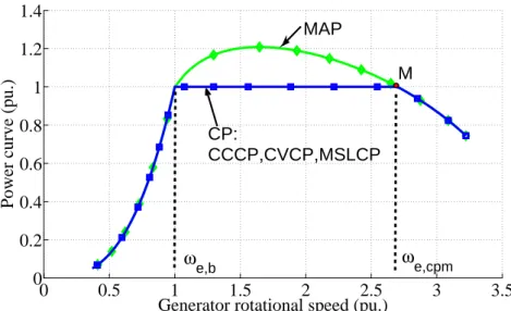
La caractéristique de fonctionnement (puissance-vitesse de rotation) d’une hydrolienne est présentée en Fig.4. Elle comprend deux zones principales: la région MPPT (Maximum Power Point Tracking) pour laquelle l’énergie extraite est maximisée jusqu’à la puissance et la vitesse de rotation nominales, puis la région dite d’écrêtage de puissance en raison des limites des organes (générateur et électronique de puissance).
0 10 20 30 40 50 60 70 0 1000 2000 3000 4000 5000
Generator mechanical rotational speed (tr/min)
Power curve (kW) ← tidal speed 4.5 m/s 3.6 m/s 2.7 m/s 1.8 m/s MAP MSLCP H(44.6, 1172) K(45.6, 1000)
Figure 4 – Courbes de puissance en mode MAP ou MSLCP
Dans la zone MPPT, pour chaque point de fonctionnement, le courant iq, à l’image du
couple, est le même quelque que soit la stratégie de commande adoptée. En sus, la commande par un convertisseur MLI autorise le réglage de id, et laisse ainsi un degré de liberté. C’est
ce degré de liberté qui permet d’implémenter des stratégies de commande différentes. Trois stratégies de commande sont étudiées: commande à facteur de puissance unitaire, commande à flux constant (tension de sortie égale à la fem) et la commande à couple max (id = 0). Chacune
montrons aussi la stratégie MSL, i.e. Minimum System Losses Control, qui calcule le courant idde façon à minimiser à la fois les pertes de la machine mais aussi celles du convertisseur. La
prise en compte des pertes convertisseur est une originalité de notre travail. Nous montrons que cette stratégie conduit à un meilleur rendement.
Ensuite, la zone de défluxage est examinée. Il s’agit de respecter des contraintes de tenue en tension et thermiques (machine et convertisseur). On distingue deux façons de procéder: travailler à la puissance maximale admissible, le système est alors en limite de tension et ther-mique ou bien maintenir la puissance constante à la valeur nominale, il y a alors une liberté sur le courant id. Dans le premier cas une seule stratégie est disponible consistant à maintenir la
tension et le courant à leurs valeurs maximales alors que la seconde autorise l’optimisation du rendement via le réglage deid. La figure ci-dessous illustre la plage de variation du courantid.
Celui-ci appartient au segment AB. Comme pour la région MPPT, deux méthodes de la littéra-ture (point A et B) sont comparées à notre algorithme qui maximise le rendement de l’ensemble convertisseur machine (point C).
iq
id −ψm
Ls
Demagnetizing current (short circuit current)
A B
C
D Current limit circle
Voltage limit circle for ωe,1
ωe,2 is the maximum speed ωe,2
ωe,j
ωe,1≤ ωe,j≤ ωe,2
id,j,optimal
iq,j (depends on torque Tj)
ˆ Vmax
ωe,jLs
Figure 5 – Illustration de la stratégie MSL
La stratégie de commande proposée en mode MPPT (MSL) et en défluxage (MSLCP) maximise le rendement de l’ensemble convertisseur machine et sera utilisée pour la suite des travaux.
11
3. Optimisation conjointe de l’ensemble machine synchrone double stator–convertisseur
On s’intéresse à l’optimisation de l’ensemble convertisseur machine en vue de minimiser l’investissement et maximiser l’énergie extraite sur une durée d’exploitation de vingt ans. L’inve -stissement est calculé à partir des coûts suivants: matières actives de la machine, la structure mécanique, et le convertisseur. L’énergie extraite est évaluée en intégrant les caractéristiques vitesse du courant marin vs puissance, vitesse du courant vs vitesse de rotation de la génératrice ainsi que les probabilités d’apparition de vitesse du courant, telles que représentées ci-dessous:
1 1.5 2 2.5 3 3.5 4 4.5 5 0 1000 2000 Mechanical power (kW) 0 50 100 150 200 250 300 350 400
Operating time in one year (h)
Tidal current speed (m/s)
1 1.5 2 2.5 3 3.5 4 4.5 50
50 100
Mechanical rotational speed (tr/min)
Power
Rotational speed Operating time
MPPT region
FW region
Rated tidal current speed
Figure 6 – Points de fonctionnement de la turbine
Afin de dégager des fronts de Pareto, un algorithme multicritère de type essaimage par-ticulaire est mis en œuvre pour d’optimiser 16 paramètres. Le modèle de la machine et du convertisseur sont ceux développés au chapitre 2 tandis que la stratégie de commande est celle proposée au chapitre précèdent (MSL).
Le front de Pareto est un guide pour le choix d’une structure, car il donne les compromis disponibles entre l’investissement et le revenu. Néanmoins, ce choix n’est pas aisé. Dès lors, nous définissons deux critères secondaires qui permettent chacun de dégager une machine par-ticulière sur le front de Pareto. La première fonction Fobj,f inal1 est calculée par la différence
entre le revenu obtenu en 20 ans et les coûts en incluant celui de la turbine estimé à 1M e. La seconde,Fobj,f inal2se détermine par le quotient des coûts par l’énergie extraite en 1 an.
Le front de Pareto obtenu est présenté Fig.7.
Ce front montre les machines A et B prédimensionnées au2ème chapitre, lesquelles sont logiquement dominées par le front de Pareto optimisé. On voit aussi apparaitre les machines déterminées parFobj,f inal1etFobj,f inal2. On pourrait croire que la meilleure machine est la plus
5.3
5.4
5.5
5.6
5.7
x 10
62
4
6
8
10
x 10
5Annual energy output (kWh)
Initial total cost(Euro)
Maximum cost, maximum energy solution Lowest cost, lowest energy solution F obj,final2 solution F obj,final1 solution Preliminary design A generator
(5.27e6, 3.08e5) Preliminary design B generator (5.31e6, 3.03e5)
Figure 7 – Pareto front
compacte, avec un grand nombre de pôles et en limite thermique (machine le plus à gauche du front). Or il n’en est rien. En effet, en passant à la machine choisie parFobj,f inal2on augmente
très légèrement l’investissement, mais on accroit de façon significative l’énergie extraite sur une durée de 20 années et donc les revenus.
On présente aussi les évolutions des paramètres (géométriques et externes) de la machine sur ce front dans l’optique de dégager des règles de dimensionnent. Par exemple, le nombre de paires de pôles est compris entre 12 et 54; la machine externe produit de l’ordre de57% de la puissance totale; la réactance unitaire est stable et très proche de80%. En outre, les paramètres des machines externes et internes sont similaires.
Une étude de sensibilité est menée sur quelques paramètres géométriques, la qualité du re-froidissement, la nature et le coût des matériaux utilisés. On montre ainsi par exemple que l’augmentation du diamètre extérieur conduit à un meilleur rendement annuel en contrepartie d’un investissement accru ou que le type de tôlerie a une faible influence sur le dimension-nement.
Une validation par la méthode des éléments finis du modèle électromagnétique analytique développé sur trois machines particuliaires du front est ensuite effectuée. Il en découle que le calcul des inductances est précis à environ 5% près et les déterminations des fem et du couple font apparaitre des erreurs de moins de1.5% et 2.0% respectivement. Notre modèle analytique donne donc une bonne estimation du comportement électromagnétique de la machine.
Enfin, nous effectuons une comparaison des résultats d’optimisation entre la machine dou-ble stator et la machine simple stator. Il apparait que la machine doudou-ble stator donne une nette amélioration du couple volumique (+65%) en contrepartie d’une légère dégradation du couple massique (-1%). Ceci permet de réduire les dimensions du générateur à attaque directe et ainsi de réduire son impact sur les écoulements du fluide. En effet, contrairement à l’éolien, le
di-13 amètre du générateur à attaque directe n’est pas négligeable devant les dimensions de la turbine hydrolienne. Un autre avantage de la structure à double stator est sa redondance naturelle.
4. Commande de la génératrice (simple ou à double stator) en mode sain ou mode dé-faut
Le dernier chapitre traite d’abord la commande de la machine synchrone simple ou à double stator en mode normal. Les stratégies de contrôle des deux convertisseurs côté machine et côté réseau sont détaillées et validés pour des conditions d’écoulement de fluide réalistes. L’accent est ensuite mis sur la commande de la DSCRPMG en mode défaut, en particulier le cas de l’ouverture d’une phase du stator externe. Trois stratégies sont élaborées et testées pour assurer une continuité de service et minimiser les ondulations de couple. La plus simple consiste à déconnecter le stator externe défaillant et fournir le couple uniquement avec le stator interne sain en tenant compte de ses limites thermiques. La2ème consiste à élaborer des consignes de courants adéquates pour le pilotage du stator défaillant et la 3ème s’appuie sur un estimateur des ondulations de couple permettant par la suite de les compenser par action sur le stator interne (Fig. 8). Ces approches sont comparées en termes de simplicité d’implémentation et efficacité de compensation des ondulations de couple montrant ainsi les possibilités offertes par la DSCRPMG. La figure 9 illustre les résultats de simulation obtenus avec la méthode basée sur l’estimateur de couple. Après compensation, le couple est quasi constant. Le taux d’ondulation de la vitesse est de l’ordre de0, 1% alors que l’oscillation de couple n’excède pas les 5%.
√ 3 3 (1 + cos 2θ) √3 3 sin 2θ Estimator ∆iq + − DSCRPMG ωm,ref + − P Idi P Iqi P Iqo P Ido + + + + + − − − P Iω k1 k2 ido iqo idi iqi ωm θ + Converter + SVPWM TL Te I∗ di I∗ qi ωm I∗ do I∗ qo εω 1 2
0.45 0.5 0.55 0.6 0.65 0.7 21.4 21.5 21.6 Speed(tr/min) Fault at 0.5s 0.45 0.5 0.55 0.6 0.65 0.7 −0.6 −0.4 −0.2 0 0.2 Torque(MN.m) 0.45 0.5 0.55 0.6 0.65 0.7 −1000 0 1000 Iabc o (A) 0.45 0.5 0.55 0.6 0.65 0.7 −1000 0 1000 Time (s) Iabc i (A) Total torque T e
Outer stator torque T
eo
Inner stator torque T
ei
Figure 9 – Performances de la DSCRPMG obtenues en mode défaut avec l’estimateur
5. Perspectives
Nous donnons ci-dessous quelques perspectives envisageables:
— Amélioration du modèle thermique: si le modèle analytique de la machine a pu être validé avec la MEF, le modèle thermique implémenté est relativement simple et nécessiterait d’être affiné et confirmé par des essais expérimentaux. Ceci est d’autant plus critique que le «rotor cup» pourrait conduire à des systèmes de refroidissement spécifiques, en particulier pour une machine de grande dimension.
— Intégration de la valeur nominale de la vitesse du courant dans le processus d’optimisation; — Etude du décalage entre les stators externes et interne en vue de réduire le cogging et/ou
les ondulations de couple;
— Prise en compte du modèle de la turbine hydrolienne dans l’étude de l’ensemble de la chaïne de conversion allant de la ressource jusqu’à l’intégration au réseau.
— Poursuivre les travaux relatifs à la tolérance aux défauts en intégrant d’autres topologies de convertisseurs.
Contents
1 State of art in tidal current energy 33
1.1 Introduction . . . 33
1.2 Tidal current resource modeling and energy extraction . . . 33
1.2.1 Tidal current principle . . . 34
1.2.2 Modeling of tidal current speed modeling . . . 35
Harmonics Analysis Method (HAM). . . 36
Practical Model (SHOM) . . . 38
1.2.3 Kinetic energy extraction . . . 39
1.2.4 Optimal regime characteristics and power curve . . . 41
Optimal regime characteristics . . . 41
Power curve. . . 42
1.3 Difference between wind energy and tidal current energy . . . 43
1.4 Hopeful turbine prototypes . . . 45
1.4.1 Horizontal axis turbine systems . . . 45
1.4.2 Ducted turbine system . . . 47
1.4.3 Vertical axis turbines system . . . 48
1.4.4 Oscillating hydrofoil turbines system . . . 49
1.5 Generator choices . . . 50
1.5.1 Squirrel cage and wound rotor induction generator . . . 50
1.5.2 Doubly fed induction generator . . . 51
1.5.3 Permanent magnet and electrically excited synchronous generator . . . 51
1.5.4 Special tidal generator researched by laboratory IREENA . . . 52
1.6 Double stator cup rotor permanent magnet generator . . . 52
1.6.1 DSCRPMG configurations . . . 54
1.6.2 DSCRPMG mechanical assembly . . . 55
1.7 Summary . . . 56
2 DSCRPMG preliminary design and control principle 57 2.1 Introduction . . . 57
2.2 Generator preliminary design Model . . . 58 15
2.2.1 Mathematical analysis of generator design model . . . 58
1). Generator main dimensions. . . 60
2). Inductance calculation . . . 64
3). Copper and iron losses model . . . 66
4). Thermal model . . . 68
5). Generator volume and mass calculation . . . 70
6). Cost model . . . 71
2.2.2 Preliminary design results . . . 71
2.3 Mathematical modeling of DSCRPMG . . . 78
2.3.1 DSCRPMG model in rotating reference frame. . . 78
2.4 Vector current control strategies in MPPT region . . . 83
2.4.1 Zero D-axis Current Control (ZDC) . . . 84
2.4.2 Unity Power Factor Control (UPF) . . . 85
2.4.3 Constant Mutual Flux Control (CMF) . . . 86
2.4.4 Minimize System Losses Control (MSL) . . . 87
2.5 Control strategies in Flux Weakening (FW) region . . . 89
2.5.1 Constant Power (CP) mode . . . 90
Constant Current Constant Power (CCCP) control . . . 91
Constant Voltage Constant Power (CVCP) control . . . 91
Minimize System Losses Constant Power (MSLCP) control . . . 94
2.5.2 Maximum Active Power (MAP) mode . . . 94
2.6 System efficiency evolution . . . 95
2.6.1 System efficiency for different control strategies in MPPT region . . . . 96
2.6.2 System efficiency for different control strategies in FW region (constant power mode) . . . 101
2.6.3 Comparison between MAP mode and CP mode . . . 103
2.7 Generators “A” and “B” cost performance comparison . . . 105
2.8 Summary . . . 107
3 Joint optimization of DSCRPMG and converter system 109 3.1 Introduction . . . 109
3.2 Optimization objectives variables and constraints . . . 111
3.2.1 Objectives. . . 112
FObj1: Maximize annual energy output . . . 112
FObj2: Minimize machine and converter cost . . . 113
Final objective 1Fobj,f inal1: Maximize revenue for 20 years . . . 113
Final objective 2Fobj,f inal2: Minimum cost energy ratio e/kW h . . . . 114
CONTENTS 17
3.2.3 Constraints . . . 115
Total cost constraint . . . 115
Geometry constraints . . . 116
Magnetic constraints . . . 117
Electrical constraints . . . 118
Winding temperature constraint . . . 118
3.3 Optimization implementation . . . 119
3.4 Results analysis . . . 121
3.4.1 Optimization parameters variation . . . 121
3.4.2 External parameters variation . . . 129
3.5 Sensibility analysis . . . 136
3.5.1 Sensibility of machine external radius . . . 136
3.5.2 Sensibility of core material type . . . 138
3.5.3 Sensibility of material unit price: Magnet, Core and Copper . . . 140
3.5.4 Sensibility of heat exchange coefficient . . . 142
3.6 Single stator and double stator PM generator comparison . . . 143
3.7 Summary . . . 146
4 PMSG and DSCRPMG system control 149 4.1 Introduction . . . 149
4.2 Gird side converter control design . . . 151
4.2.1 Outer loop control design. . . 153
4.2.2 Inner loop control design . . . 154
4.2.3 Grid side control simulation results . . . 155
4.3 Generator side control in normal condition . . . 156
4.3.1 Control structure of PMSG . . . 156
PMSG inner current loop controller design . . . 157
PMSG outer speed loop controller design . . . 159
4.3.2 Control structure of DSCRPMG . . . 161
Inner current loop controller design of DSCRPMG . . . 163
Outer speed loop controller design of DSCRPMG. . . 163
4.3.3 Simulation results of generator (PMSG and DSCRPMG) side control in normal conditions . . . 166
4.4 PMSG and DSCRPMG control in fault conditions . . . 171
4.4.1 Control of PMSG in the condition of open circuit fault . . . 172
4.4.2 Control of DSCRPMG in the condition of open circuit fault . . . 174
Method 2: Control the generator by changing the faulty stator current control references . . . 177 Method 3: Control the generator by changing the two stator current
references with compensator or estimator . . . 180 4.4.3 Comparison between the faulty control methods. . . 186 4.5 Summary . . . 187
5 Conclusions & perspectives 189
5.1 Conclusions . . . 189 5.2 Perspectives . . . 191
Appendices 193
Appendix A Converter losses model 195
A.1 Conduction losses . . . 195 A.2 Switching losses. . . 196
Appendix B Principle of particle swarm optimization 199
Appendix C Analytical model validation by FEMM 201
C.1 Flux density, torque and inductance verification . . . 201 C.2 Post calculation of non-integer number of conductor per slot . . . 205
Appendix D Generator Simscape codes 209
D.1 DSCRPMG code . . . 209
Appendix E Control parameters 215
E.1 Optimized DSCRPMG parameters (Generator choosing from the Pareto front in Chater 3 with criteriaFobj,f inal2) . . . 215
E.2 Optimized PMSG parameters and corresponding controller parameters (Gener-ator choosing from the Pareto front in Chater 3 with criteriaFobj,f inal2) . . . 216
List of Symbols
β Turbine blades pitch adjustment angle, °; The magnet arc angle, °.
ǫ Short pitching.
γ The ratio between coil pitch and pole pitch. ˆ
Bg Air-gap max fundamental flux density,T.
ˆ
Bm Maximum flux density,T.
ˆ
Bs Saturation flux density,T.
κc Carter coefficient.
λ Tidal current turbine tip speed ratio.
λs The slot permeance factor.
λs Tooth tip permeance factor.
µo The permeability of free space,H/m.
µrm The permeability of magnet,H/m.
ωe Electrical rotational speed of generator,rad/s.
ωm Mechanical rotational speed of turbine rotor,rad/s.
ωe,b Base (rated) electrical rotational speed of generator,rad/s.
Φz Common factor of tides harmonics.
ψP M The max fundamental flux in the air gap,Wb.
ρ The density of tidal current,kg/m3.
ρcu The electrical resistivity of copper,Ω/m.
σz Circular frequency of tides,Hz.
τd The tooth pitch,m.
τp Pole pitch,m.
θele Electrical angle, °.
ϕ Power factor angle, °.
A The electric linear current loading,A/m.
Az Amplitude of tides harmonics,m.
Br Magnet remanence,T.
C Tide coefficient; Cost of material, e.
Cp Tidal power coefficient.
Cz Latitude factor of tides harmonics.
d Density of material,kg/m3.
Do Bore diameter of the outer stator lamination,m.
E RMS value of the stator fundamental induced EMF,V.
Etidal Kinetic energy contained in the tidal current,J.
f Frequency of a synchronous generator,Hz.
g Gravitational acceleration,m/s2.
H Height of the tides,m.
h Heat exchange coefficient,W/m2K.
H0 Mean sea level,m.
hm The thickness of the magnet,m.
hr The thickness of rotor,m.
hslot The height of slot,m.
hyoke The thickness of yoke,m.
i Phase current,A.
id,q The current in d and q axis,A.
Is RMS value of the stator nominal RMS phase current,A.
J Current density,A/mm2; Rotor inertia,kg m2.
j Tidal turbine operation point number.
kf The winding fill factor.
kh The specific loss coefficients for hysteresis.
KL Effective loss coefficient of the channel; Coefficient for end winding.
KT Turbine quantity coefficient.
kt The teeth open ratio.
kd1 Winding distribution factor of the fundamental harmonic.
kec The specific loss coefficients for eddy currents.
kF e Iron lamination factor.
kp1 Winding pitch factor of the fundamental harmonic.
kw1 Winding factor of the fundamental harmonic.
L Length of the stator lamination,m.
Lσ Air-gap leakage inductance,H.
lg Mechanical air-gap length,m.
Ld,q Direct-axis and quadrature-axis inductance,H.
Lef f Effective machine length,m.
Lmd,mq The direct-axis and quadrature axis magnetizing inductance,H.
CONTENTS 21 Lslot Slot leakage inductance,H.
Ltooth Tooth tip leakage inductance,H.
M Mass of material,kg.
m Number of slots per pole per phase.
N Number of turns per phase.
n Turbine rotor turning speed,r/min; The order of the harmonics.
Nc Number of conductors in one slot.
P Extracted power from tidal power,W.
p The number of pole pairs.
Pi Inner stator power of the generator,W.
Pn Total power of the generator,W.
Po Outer stator power of the generator,W.
Pconv Converter losses,W.
Pculoss Total copper power loss,W.
Piron Total core power loss,W.
Ptidal Power of tidal current,W.
q The number of phase.
Qs The number of slots.
R The generator outer surface radius,m.
Rb Turbine blades radius,m.
Rcu Winding resistance for one phase,Ω.
Rshaf t Generator shaft radius,m.
Rso Bore radius of the outer stator lamination,m.
S Rotational area of turbine blades,m2.
Sd Heat exchange surface,m2.
Si Inner stator apparent power,VA.
So Outer stator apparent power,VA.
Scu The surface of copper conductor,m2.
t Time,s.
TA Ambient temperature, °C.
Te Electric torque,Nm.
TL Turbine torque,N m.
Tcu Winding temperature, °C.
Tiron Iron temperature, °C.
V Tidal current volume pass through the turbine blades or volume of material, m3; Root mean square value of phase terminal voltage,V.
v Phase voltage,V.
vc Cut-out or Furling tidal speed,m/s.
vi Cut-in tidal speed,m/s.
vr Rated tidal speed,m/s.
vt Tidal current velocity,m/s.
Vz Initial phase of tides whent = 0, rad.
vd,q The voltage in d and q axis,V.
vf i The surface tide velocity,m/s.
Vnt Neap tide current velocities,m/s.
Vst Spring tide current velocities,m/s.
vth Theoretical tide velocity,m/s.
Vtide Tidal current velocity for a choosing site ,m/s.
wslot The width of slot,m.
Acronyms
Symbol Description
CCCP Constant Current Constant Power
CMF Constant Mutual Flux
CP Constant Power
CVCP Constant Voltage Constant Power
DC Direct Current
DSCRPMG Double Stator Cup Rotor Permanent Magnet Generator
FEA Finite Element Analysis
FEMM Finite Element Method Magnetics
FW Flux Weakening
MAP Maximum Active Power
MML Minimize Machine Losses
MOPSO Multi-Objective Particle Swarm Optimization
MPPT Maximum Power Point Tracking
MSL Minimize System Losses
MSLCP Minimize System Losses Constant Power
PMSG Permanent Magnet Synchronous Generator
UPF Unity Power Factor
List of Tables
1.1 Principal tidal harmonic constituents . . . 37 1.2 Supposed tidal current location project parameters . . . 43 1.3 Comparison of the differences between wind turbine and tidal turbine . . . 44 1.4 Main projects of horizontal axis turbines . . . 47 1.5 Main projects of ducted turbines . . . 48 1.6 Main projects of vertical axis turbines . . . 49 1.7 Main projects of oscillating hydrofoil turbines . . . 49 2.1 Constant parameters used in the model . . . 59 2.2 Analytical expressions for the machines basic dimensions . . . 72 2.3 A and B generator performance comparison at rated power . . . 78 2.4 Control parameters of generator “A” . . . 95 2.5 Summary of the different control strategies (ZDC, CMF, MML, MSL) in MPPT
region for the generator “A”. . . 99 2.6 Generator “A”: Base operation point current and voltage.Sconvare the minimum
apparent needed for corresponding control strategies. ˆImax = q
i2
d,b+ i2q,b and ˆ
Vmax =p(−ωeLqiq,b)2+ (ωeψP M + ωeLdid,b). . . 99
2.7 Generator “A”: Maximum CP speed and maximum operational speed of generator100 2.8 Summary of the different control strategies (CCCP, CVCP, MSLCP) for FW
region with CP mode. . . 103 2.9 Control parameters of generator “B” . . . 106 2.10 Converter size to have complete CP range for generator “A”.Sconvare the
min-imum apparent needed to have full range MSLCP control. . . 106 2.11 Converter size to have complete CP range for generator “B”.Sconvare the
min-imum apparent needed to have full range MSLCP control. . . 107 3.1 Optimization parameters. . . 115 3.2 The parameter changes of the lowest cost solution (“Traditional dimensioning
generator”), Fobj,f inal2: minimum cost energy ratio,Fobj,f inal1: maximum
rev-enue solution and maximum energy solution. . . 124 23
3.3 Summarize of the optimized parameters variation trends . . . 129 3.4 Comparison between the optimization results and their corresponding values in
literature. . . 136 3.5 Typical values of convection heat exchange coefficients. . . 142 3.6 Sensibility index of external diameterR, core type, material unit price and heat
exchange coefficienthc. . . 143
3.7 Single stator generator optimization parameters. . . 144 4.1 Fault tolerant control performance comparison. M: Method. WTL: Winding
Temperature Limit. RI: Reconfiguration Implement . . . 186 C.1 Parameters of the three generators. . . 202 C.2 Series non-integer conductor number change to integer conductor number . . . 202 C.3 Lowest cost,Fobj,f inal2andFobj,f inal1 solution inductance comparison between
analytical method and finite element method . . . 205 E.1 Optimized DSCRPMG parameters and relatively controller parameters which
are used to test the fault control. . . 215 E.2 Optimized PMSG parameters and relatively controller parameters which are
used to test the fault control. . . 216 E.3 Grid side control parameters and torque estimator parameter. . . 216
List of Figures
1 Structure d’une chaine hydrolienne à base de génératrice synchrone à double stator . . . 6 2 Connexion des 2 stators au même bus DC . . . 8 3 Paramètres géométriques de la machine synchrone double stator étudiée . . . . 8 4 Courbes de puissance en mode MAP ou MSLCP . . . 9 5 Illustration de la stratégie MSL . . . 10 6 Points de fonctionnement de la turbine . . . 11 7 Pareto front . . . 12 8 Commande de la DSCRPMG en mode défaillant, méthode avec estimateur . . . 13 9 Performances de la DSCRPMG obtenues en mode défaut avec l’estimateur . . 14 1.1 Formation of tides . . . 35 1.2 Tides channel model . . . 37 1.3 Tidal velocity example (HAM) . . . 38 1.4 Tidal velocity example (SHOM) . . . 39 1.5 Relationship betweenCp,λ and β . . . 40
1.6 Optimal regime characteristics . . . 41 1.7 Theoretical power and speed curve for a fixed pitch turbine with power limitation 42 1.8 Induction generator topology . . . 50 1.9 DFIG topology . . . 51 1.10 Synchronous generator topology . . . 51 1.11 Doubly salient permanent magnet generator . . . 53 1.12 Two stators are connected independently to DC-bus . . . 53 1.13 Radial-flux double stator PM generator configuration . . . 54 1.14 3D mechanical assembly illustration of a simple DSCRPMG . . . 55 2.1 Double stator permanent magnet machine structure . . . 58 2.2 Approximately air gap flux density for surface mounted magnet generator . . . 62 2.3 Double-layer winding slot tooth dimensions . . . 66 2.4 SURA-M400-50A loss curve fitting . . . 68 2.5 Efficiency and losses variation . . . 72
2.6 Current density varying withRso . . . 73
2.7 Cost of generator varying withRso . . . 73
2.8 Generator length varying withRso . . . 74
2.9 Torque active mass density . . . 74 2.10 Torque volume density . . . 75 2.11 Inductance varies with the outer bore radiusRso . . . 75
2.12 Inductance varies with the ratio between slot height and slot width . . . 76 2.13 Ratio between armature and permanent magnet flux linkage. . . 76 2.14 Phasor-diagram for PM machine with different inductance . . . 77 2.15 Iron and winding temperature varying withRso . . . 77
2.16 Generator A flux lines with load current . . . 81 2.17 Vector diagram of non-salient PM generator with ZDC control . . . 85 2.18 Vector diagram of non-salient PM generator with UPF control . . . 85 2.19 Vector diagram of non-salient PM generator with CF control . . . 87 2.20 Illustration of minimize system losses control strategy . . . 89 2.21 CP and MAP mode in FW region. Three control strategies (CCCP,CVCP,MSLCP)
are presented in CP mode . . . 90 2.22 MAP and CVCP trajectory. . . 92 2.23 Classical power torque curve of tidal current turbine . . . 95 2.24 System efficiency operated with different control strategies in MPPT region . . 96 2.25 Copper losses in MPPT region under different control strategies . . . 97 2.26 Iron losses in MPPT region under different control strategies . . . 98 2.27 Converter losses in MPPT region under different control strategies . . . 98 2.28 Power factor in MPPT region under different control strategies . . . 99 2.29 Generator “A”: Extractable power curve for different control strategies with the
minimum needed converter rated current and voltage which are calculated at base (rated) operation point respectively. . . 100 2.30 System efficiency operated with different control strategies in FW region(CP
mode) . . . 101 2.31 Copper losses in FW region under different control strategies(CP mode). . . 102 2.32 Iron losses in FW region under different control strategies(CP mode). . . 102 2.33 Converter losses in FW region under different control strategies(CP mode). . . 103 2.34 Power curve for MAP and MSLCP . . . 104 2.35 Efficiency comparison of MAP and MSLCP . . . 105 2.36 Machine losses in FW region of MAP and MSLCP . . . 105 2.37 Generator “A” and “B” efficiency comparison . . . 107 3.1 Turbine operating points . . . 110
LIST OF FIGURES 27 3.2 Example of Pareto front optimal points (represented by circles) and a dominated
point (represented by a cross). . . 112 3.3 Optimization flow chat . . . 120 3.4 Pareto front and four extreme solution generator shapes . . . 123 3.5 Final objective 1: Evolution of 20 years revenue vs. objectives. Red point:
maximize the 20 years revenue design solution; Magenta point: minimum cost energy ratio design solution. . . 124 3.6 Final objective 2: Cost energy ratio e/kW h vs. objectives. Red point:
maxi-mize the 20 years revenue design solution; Magenta point: minimum cost en-ergy ratio design solution.. . . 125 3.7 Evolution of optimization parameters k1, p, kt andRso vs. the two objectives.
Red point: maximize the 20 years revenue design solution; Magenta point: min-imum cost energy ratio design solution. . . 126 3.8 Evolution of optimization parametershyokeo andhyokei, hslotoandhsloti,lg and
hm vs. the two objectives. Red point: maximize the 20 years revenue design
solution; Magenta point: minimum cost energy ratio design solution. . . 127 3.9 Evolution of optimization parametershr andL, Nsloto,Nsloti,Sconvo,Sconvivs.
the two objectives. Red point: maximize the 20 years revenue design solution; Magenta point: minimum cost energy ratio design solution. . . 128 3.10 Evolution of no load fundamental peak air gap flux density vs. objectives. Red
point: maximize the 20 years revenue design solution; Magenta point: mini-mum cost energy ratio design solution. . . 130 3.11 Evolution of generator active mass and torque mass density, volume and torque
volume density vs. objectives. Red point: maximize the 20 years revenue de-sign solution; Magenta point: minimum cost energy ratio dede-sign solution. . . . 132 3.12 Evolution of max winding temperature vs. objectives. Red point: maximize the
20 years revenue design solution; Magenta point: minimum cost energy ratio design solution. . . 133 3.13 Evolution ofA × J vs. objectives. Red point: maximize the 20 years revenue
design solution; Magenta point: minimum cost energy ratio design solution. . . 133 3.14 Evolution of annual power losses and annual efficiency vs. objectives. Red
point: maximize the 20 years revenue design solution; Magenta point: mini-mum cost energy ratio design solution. . . 134 3.15 Evolution of LsIrated to ψP M ratio vs. objectives. Red point: maximize the
20 years revenue design solution; Magenta point: minimum cost energy ratio design solution. . . 135
3.16 Evolution of different part cost vs. objectives. Red point: maximize the 20 years revenue design solution; Magenta point: minimum cost energy ratio design solution. . . 135 3.17 Sensibility comparison between external radiusR = 1.5m and R = 3m . . . . 137 3.18 SURA-M800-65A loss curve fitting . . . 138 3.19 Sensibility comparison between core type M800-65A and M400-50A . . . 139 3.20 Sensibility comparison between different material unit price . . . 141 3.21 Sensibility comparison between different heat exchange coefficient . . . 143 3.22 Conventional single stator PM generator structure . . . 144 3.23 Double stator and single stator PM generator optimization evolution comparison.145 3.24 Ratio between blade diameter and generator diameter for wind turbine and tidal
current turbine. . . 146 4.1 PMSG system . . . 150 4.2 DSCRPMG system . . . 150 4.3 Control structure of the grid side converter . . . 151 4.4 Grid side control simulink blocks . . . 155 4.5 Grid side control simulation results . . . 156 4.6 Control scheme of PMSG side converter . . . 157 4.7 q-axis current control loop . . . 157 4.8 d-axis current control loop . . . 158 4.9 Bode diagram of the q-axis current loop . . . 159 4.10 Speed control loop of PMSG . . . 159 4.11 Step response of inner current and speed control loop of PMSG . . . 160 4.12 Bode diagram of the speed control loop of PMSG . . . 161 4.13 Control scheme of DSCRPMG side converter. k1 is the outer stator power
per-centage of the total power; k2 is the inner stator power percentage of the total
power. . . 162 4.14 Speed control loop structure of DSCRPMG . . . 164 4.15 Step response of inner current loop and outer speed loop . . . 165 4.16 Bode diagram of the speed control loop of DSCRPMG . . . 165 4.17 PMSG in healthy condition . . . 166 4.18 DSCRPMG in healthy condition . . . 167 4.19 PMSG operation simulation in health and variable speed conditions . . . 169 4.20 DSCRPMG operation simulation in health condition and variable speed conditions170 4.21 Open circuit fault illustration . . . 171 4.22 Vector control strategy of PMSG under open circuit fault condition . . . 173 4.23 Single stator performance in health and open circuit fault control. . . 174
LIST OF FIGURES 29 4.24 Method 1: Fault control method through shunting down the fault stator . . . 176 4.25 Winding temperatures variation with the speed and current of the selected DSCRPMG.177 4.26 Control structure of of DSCRPMG in fault condition: Modify the current
refer-ence of the failure stator . . . 178 4.27 Method 2: Faulty control method through only modifying the faulty stator
cur-rent control references . . . 179 4.28 Proposed fault control diagram using high pass filter based compensator. . . 181 4.29 Method 3: Fault control method by modifying outer stator current references
and using high pass filter based compensator . . . 182 4.30 Proposed fault control diagram using torque estimator. . . 183 4.31 Estimator structure . . . 184 4.32 Method 3: Fault control method by modifying outer stator current references
and using torque estimator . . . 185 C.1 Lowest investment design solution . . . 203 C.2 Fobj,f inal2design solution . . . 203
C.3 Fobj,f inal1design solution . . . 204
C.4 Simple illustration and comparison for non-integer conductor post calculation . 207 D.1 Simscape DSCRPMG model connect with Simpowersystem . . . 210 D.2 DSCRPMG parameters setting mask . . . 210
Introduction
There is worldwide agreement on the need to reduce greenhouse gas emissions, and differ-ent policies are evolving both internationally and locally to achieve this. This kind of world trend drives people to explore different kinds of renewable energy such as wind power, solar power and ocean power. Wind power and solar power have been industrialized and successfully integrated to the grid in large scale for many years. More and more organizations, companies and laboratories start to focus on exploring ocean power. More than 70% of the earth area is covered by ocean and in which stored a vast of energy. The oceans represent an energy resource which is theoretically far larger than the entire human race could possibly use. The existed vari-ous forms in ocean power are namely tidal rise & fall energy, tidal (ocean) current energy, wave energy, salinity gradient and thermal gradient energy. Among them, tidal current energy1 has obtained a strong increasing interest due to the advantages of predictable, high power density and huge potential characteristics in the last decade.
Tidal current energy has been regarded as the most closely commercialized resource and the method to harness tidal current energy has some similarities with wind power technology. An abundant of tidal current turbines have been originally designed by different universities and industries. Some of them have realized to transfer electricity to the customer. In Europe, many countries and company are scheduled to build several megawatt range tidal current energy farm and to supply electricity for coastal areas or remote islands in the near coming future. However, there are still some difficulties before commercialization in large scale of the tidal current energy system. The investment cost of tidal current energy is still very high comparing with wind energy even with the tax deduction and exemption by government. This thesis work mainly focuses on two sides to improve the tidal current energy system cost performance which are generator optimization design and fault tolerant control. Fixed pitch direct drive system with Double Stator Cup Rotor Permanent Magnet Generator (DSCRPMG) is adopted in this thesis. Fixed pitch system is robust and provides less power oscillation. Direct drive system eliminates the gear-box which may lead high maintenance cost and long downtime. As the tidal current speed profile is predictable for a selected tidal site for a long term, DSCRPMG design will take full consideration of the operation point and its corresponding operation time. Fault tolerant control is researched to reduce the system downtime.
1. It is also called marine current energy or ocean current energy
The structure of this thesis is:
— The first chapter presents the state of art of tidal current energy. Tidal current source modeling and power extracting are briefly discussed. The up to date hopeful tidal turbines are shown in the classification of tidal turbine type. The advantages and disadvantages of the possible generator system for tidal current energy application are also summarized. Some introductions of the researched double stator PM generator are given at the end of this chapter.
— The second chapter discusses the design of a DSCRPMG at the rated power condition. Then, a comprehensive comparison of different current vector control strategies are made through evaluating the generator converter system efficiency both in Maximum Power Point Tracking (MPPT) region and Flux Weakening (FW) region. Several control strate-gies (zero d-axis current control (ZDC), constant mutual flux (CMF) and minimize ma-chine loss (MML)) are analysed and compared. An approach minimising all system loss (machine and converter) and allowing to maximise efficiency is adopted.
— The third chapter presents a methodology of DSCRPMG optimization design which takes into account the control strategy and predicted tidal current frequency into consideration using Multi-Objective Particle Swarm Optimization (MOPSO) tool. 16 variable parame-ters including DSCRPMG geometry parameparame-ters and converter size parameparame-ters are to be optimized under the mechanical, magnetic, electrical and thermal constraints. The two optimization objectives are maximizing the annual energy output and minimizing the in-vestment for the specific tidal energy site. Comparison between PMSG and DSCRPMG optimization design for the same turbine and torque speed profile are discussed in this chapter.
— The fourth chapter researches the control system design of PMSG and DSCRPMG for health and open circuit fault conditions. The health condition operation systems are firstly designed. The performances under constant tidal speed or variable tidal speed are pre-sented and discussed. In the open circuit fault condition, three control strategies are proposed for DSCRPMG to remedial the torque and speed oscillation. The results show that DSCRPMG system has much better fault tolerant performance than PMSG system. — The final chapter is the general conclusion and perspective of this thesis.
1
State of art in tidal current energy
extracting technologies
1.1
Introduction
The potential of electric power generation from tidal currents is enormous. Tidal currents are being recognized as a resource to be exploited for the sustainable generation of electrical power. The high ocean water density leads to that tidal current turbine blades size are much smaller than wind turbine blades for the same power level. Additionally, tidal source is highly predictable for long time. Those characteristics make tidal current extremely promising and advantageous for power generation when compared to other renewable energy resources. The technology used for harnessing tidal current energy mainly based on the relevant work which has been carried out on ship’s propellers, wind turbines and on hydro turbines. This chapter reports tidal power fundamental concepts and two currently used source modeling methods. The most promising tidal turbine projects worldwide are classified depending on the structure of turbine and some brief notes are given. The possible generator choices and system topologies are presented. Furthermore, the introduction of the researched DSCRPMG characteristics are briefly introduced.
1.2
Tidal current resource modeling and energy extraction
The technologies used to extract most of renewable energy are closely depending on the characteristics of the resource. Undoubtedly, some basic understanding of the resource
namics is therefore one of the first steps to be considered before exploiting it. This section will discuss the formation reasons and model methods of tidal current firstly and then the tidal power harness principles.
1.2.1
Tidal current principle
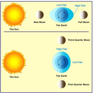
The global tidal current or marine current energy resources are the horizontal movement of water mostly driven by tides which caused by gravitational interactions between sun, moon, and earth. In some cases the tidal currents are also caused by thermal gradient and salinity gradient effects. The tides can be classified into three types: semi-diurnal, diurnal and mixed tide. Semi-diurnal tide causes water to flow both inwards (flood tide) and seawards (ebb tide) twice each day with a cycle period approximately 12 hours and 24 minutes. Diurnal tide flows once both inwards and seawards each day with a cycle period approximately 24 hours and 48 minutes. Mixed tide is a combination result of the semi-diurnal and diurnal effects and which is the most dominant type in the world. Tides are generated by gravitational forces of the sun and moon on the ocean waters of the rotating earth. The strength of the currents varies, depending on the distance of the moon and the sun relative to the earth. The magnitude of the tide-generating force is about68% moon and 32% sun due to their respective masses and distance from Earth. The sun’s and moon’s gravitational forces create two “bulges” in the earth’s ocean waters: one directly under or closest to the moon and other on the opposite side of the earth. These “bulges” are the two tides a day observed in many places in the world. Unfortunately, this simple concept is complicated by the fact that the earth’s axis is tilted at 23.5 degrees to the moon’s orbit; the two “bulges” in the ocean are not equal unless the moon is over the equator. This difference in tidal height between the two daily tides is called the diurnal inequality or declination tides and they repeat on a14 day cycle as the moon rotates around the earth. Where the semi-diurnal tide is dominant, the largest marine currents occur at new moon and full moon (high tides), which is when the sun and moon’s gravitational pull are aligned. The lowest, occurs at the first and third quarters of the moon (low tides), where the sun and moon’s gravitational pull are 90 degrees out of phase as shown in Fig. 1.1 [1]. With diurnal tides, the current strength varies with the declination of the moon (position of the moon relative to the equator). The biggest currents appear at the extreme declination of the moon and lowest currents at zero declination. Therefore differences in currents occur due to changes between the distances of the Moon and Sun from Earth, their relative positions with reference to Earth and varying angles of declination. These positions occur with a periodicity of two weeks, one month, one year or longer, and are entirely predictable [2]. This means that the strength of the tidal currents generated by the tide varies, depending on the position of the site on the earth. Other factors such as the shape of the coastline and the bathymetry (shape of the sea bed) also affect the strength of tidal currents. Along straight coastlines and in the middle of deep oceans, the tidal
1.2. TIDAL CURRENT RESOURCE MODELING AND ENERGY EXTRACTION 35
Figure 1.1 – Formation of tides
range and marine currents are typically low.
To estimate one location whether it is suitable to build a tidal turbine farm or not, the resource should be assessed thanks to oceanographic databases. The main key criteria are: maximum spring current velocity; maximum neap current velocity; seabed depth; maximum probable wave height in 50 years; seabed slope; significant wave height; and the distance from land [3] [4].
1.2.2
Modeling of tidal current speed modeling
Tides and tidal current are periodically in motion as a result of Sun-Moon-Earth gravitational system interaction. In fact, it is not easy to get the exact behavior. In any hydrodynamic model for tidal current flow in a channel, there is a requirement for accurate water height data and channel parameters. For any subsequent resource evaluation and site capacity estimation there must be a large amount of data available (usually at least 1 year). Currently, there are several ways to model the tidal current velocity. At the same time, the modeling of the tidal channel is also very important. Different shape of channel change tidal current velocity sharply. All of the model methods depend on the marine meteorology data measured in the past years. In this part we will mainly present two method called Harmonics Analysis Method (HAM) and Practical Model (SHOM)1(French Navy Hydrographic and Oceanographic Service, Brest, France) [5].
There are also other kinds of methods to simulate tidal current model such as Tide 2D and Double Cosine Method [6].
Harmonics Analysis Method (HAM)
The tide change at any location can be divided into many tidal harmonic constituents (partial tides), then calculate the tidal amplitudes and phases of each partial tide according to the tidal observations. Tide can be considered as a superposition of many simple waves. This method is usually called Harmonics Analysis Method (HAM). Each single simple wave corresponds to an object called imaginary celestial body. So the whole tide caused by the tidal force can be written as [6,7]: H = Cz X z AzΦzcos(σzt + Vz) (1.1) Where:
H: Height of the tide (m);
σz: Circular frequency (rad/hour);
t: Time (hour);
Vz: Initial phase (rad) whent = 0;
Cz: Latitude factor;
Φz: Common factor;
Az: Amplitude (m);
In order to build the tidal current model, there are 11 very important harmonic tides needed: — 4 semi-diurnal partial tides: M 2 (Principal Lunar Semi-diurnal Constituent), S2 (Princi-pal Solar Semi-diurnal Constituent),N 2 (Large Lunar Elliptic Semi-diurnal Constituent), K2 (Luni-solar Semi-Diurnal Constituent);
— 4 diurnal partial tides: K1 (Luni-solar Diurnal Constituent), O1 (Principal Lunar Diurnal Constituent),P 1 (Principal Solar Diurnal Constituent), Q1 (Large Lunar Elliptic Diurnal Constituent);
— 3 shallow water constituents (due to the topography and effect of interference): M 4 (Lu-nar 1/4 Diurnal Shallow Water Constituent),M S4 (Lunisolar 1/4 Diurnal Shallow Water Constituent),M 6 (Lunar 1/4 Diurnal Shallow Water Constituent).
The initial phaseVz, AmplitudeAz and factors depend on the choosing site.
Approximately, choosing some of the very important harmonic tides to build the tidal current model we can acquire relatively high accuracy. In order to simplify the equation Eq.1.1and the calculation, we just choose some of the tides: M 2, N 2, S2, K1, O1, M 4 and M 6 and their values are shown in Table.1.1. Then the whole formulation Eq.1.1 for the tide height can be rewritten as follow: H(t) =H0+ AM 2cos(σM 2t + VM 2) + AN 2cos(σN 2+ VN 2) + AS2cos(σS2t + VS2) + AK1cos(σK1t + VK1) + AO1cos(σO1t + VO1) + AM 4cos(σM 4t + VM 4) + AM 6cos(σM 6t + VM 6) (1.2)
1.2. TIDAL CURRENT RESOURCE MODELING AND ENERGY EXTRACTION 37
z Harmonic Constituent Definition σz(rad/hour)
M 2 Principal Lunar Semi-diurnal 0.5059
N 2 Large Lunar Elliptic Semi-diurnal 0.4964
S2 Principal Solar Semi-diurnal 0.5236
K1 Luni-solar Diurnal 0.2625
O1 Principal Lunar Diurnal 0.2434
M 4 First overtide ofM 2 1.0117
M 6 Second overtide ofM 2 1.5176
Table 1.1 – Principal tidal harmonic constituents
H(t)=mean sea level + contribution from sum of harmonic constituents; Where: A is the amplitude of each harmonic constituent; H0 is mean sea level.
As the tidal height is predicted by specific method, such as HAM mentioned above, it allows us to deduce the tidal current velocity. It should be noticed that the velocity of the tidal current is the final key criteria to assess tidal current location. Tidal currents flow in channel. Each channel is of course unique in terms of its width and depth variations, roughness etc. The basic premise of the channel model method is therefore to take a real channel and idealize it into a simple mathematical model. Water height level data from two reservoirs on either end of the channel need to be obtained. The tidal height at the first reservoir is at a heighth1and the second
is at a height h2. A Side-view and a top-view of the channel model are shown in Fig.1.2. So
h1 h2 Inlet height length l Outlet height Width w
Figure 1.2 – Tides channel model the theoretical tide velocity is:
vth=p2g|(h1− h2)| (1.3)
Whereg is gravitational acceleration equal to 9.8m/s2, h
1 andh2 can be calculated by Eq.1.2
with a constant time difference between two tide height. But, due to the Law of Conservation of Mechanical energy and take into account the effect of material in the seabed as well as effect of channel blockage [6], the final velocity equation can be written as:
vf i =
s
2g|(h1− h2)|
1 + KL+ KT
(1.4)
0 100 200 300 400 500 600 700 800 −4 −3 −2 −1 0 1 2 3 4 Time(hour) Tide Velocity(m/s)
Tidal Velocity in hours
Figure 1.3 – Tidal velocity example (HAM)
which represented in terms of number of turbines. Something should be emphasized is that vf iis the surface tidal current velocity. The calculation methods of the coefficientKLandKT
are showed in the literature [6]. Fig. 1.3 shows the HAM simulation result for the choosing tidal harmonics parameter. This method is used to model a tidal current speed for the following generator design Chapter. Once the tidal current speed profile is obtained, the tidal current speed frequency is consequently obtained. The generator optimization design will take this tidal speed frequency into consideration.
Practical Model (SHOM)
The tidal current data used in this method is provided by the SHOM [8]. For a specific site, it needs the current velocities for spring and neap tides. These values should be given at hourly intervals starting at 6 hours before high waters and ending 6 hours after. Therefore, knowing tide coefficients, it is easy to derive a simple and practical model for tidal current velocitiesVtide
as follow:
Vtide = Vnt+(C − 45)(Vst− Vnt
)
95 − 45 (1.5)
WhereC is the tide coefficient which characterize each tidal cycle (95 and 45 are respectively the spring and neap tide medium coefficient). The value of tide coefficientC for different France tidal locations can be find on the website [8]. This coefficient is determined by astronomic calculation of earth and moon positions. Vst and Vnt are respectively the spring and neap tide
current velocities for hourly intervals starting at 6 hours before high waters and ending 6 hours after. For example, 3 hours after the high tide, Vst = 1.8 knots andVnt =0.9 knots. Therefore,
1.2. TIDAL CURRENT RESOURCE MODELING AND ENERGY EXTRACTION 39 0 100 200 300 400 500 600 700 −5 −4 −3 −2 −1 0 1 2 3 4 Time(hour) Tidal velocity(m/s)
Figure 1.4 – Tidal velocity example (SHOM)
for a tide coefficientC=80, Vtide=1.53 knots. However,this method is the ideal current velocity
model. In practice, the speed of the tidal current will fluctuates with swells which are considered as the main disturbance of the tidal current velocity. Normally, high tidal speed sites are often located at shallow water sites with typical sea depth about 30-50m. And for this depth the fluctuation caused by underwater propagation of swells can not be negligible when use SHOM method to model the tidal current velocity. The author (Zhibin Zhou) discussed the power fluctuation caused by the influence of swells and the modeling method of swells in detail [9]. Fig.1.4shows the SHOM simulation result for tidal location Penmarc’h, France in Sept.2011.
1.2.3
Kinetic energy extraction
The energy in the tidal current is in the form of kinetic energy like wind power. Kinetic energy contained in the tidal current is characterized by the equation:
Etidal =
1 2mv
2
t (1.6)
Where the mass of tidal currentm = ρV , ρ is the density of the ocean water (1025kg/m3) and
V = Svtt is the tidal current volume pass through the turbine blades in time t. vt is the tidal
current velocity andS is rotational area of turbine blades. For the chosen turbine blades radius Rb, so the turbine blades swept area S = πRb2. Consequently the power of the water flow is
given by: Ptidal= Etidal t = 1 2ρSv 3 t (1.7)
The kinetic energy contained in tidal current can’t be totally extracted by the turbine blades because the tidal current on the back side of the blades must have a high enough velocity to move away and allow more tidal current flow through the plane of the blades. The question that how much of the tidal energy can be transferred to the blade as mechanical energy has been answered by the Betz’law. Betz’law states that only a maximum of 59.25% of the kinetic power in the fluid can be converted to mechanical power using turbine blades. That number is the so called maximum power coefficient or Betz-Number.
The ratio between the rotor blades extracted powerP and the power contained in the tidal currentPtidalis given by the power coefficientCp:
Cp =
P Ptidal
(1.8) Cp is a function of tip speed ratioλ and turbine blades pitch adjustment angle β. The tip speed
ratio is defined as:
λ = Rbωm vt
(1.9) Whereωm(rad/s) is the mechanical rotational speed of rotor. Fig. 1.5 is an example to show
0 2 4 6 8 10 12 14 16 0 0.1 0.2 0.3 0.4 0.5 0.6 β=0°
Tip speed ratio, λ
C p β=0° β=2° β=6° β=10° β=14° β=18°
Figure 1.5 – Relationship betweenCp,λ and β
the characteristics of one turbine [10]. For every pitch angleβ, there is a tip speed ratio λ which corresponds to the maximum power coefficient and hence the maximum efficiency. It can be seen that the power efficiency significantly depends on the pitch angle and the tip speed ratio. Therefore, the pitch angle of the blade has to be changed mechanically in respect to the actual tip speed ratio in order to capture maximum tidal power. This is the theoretical basis for the tidal power maximum efficiency controlling. Cpcurve is strongly dependent on the production