Faible complexité et haute performance de la transformée de Fourier

UNIVERSITÉ DU QUÉBEC

THÈSE PRÉSENTÉE À

L'UNIVERSITÉ DU QUÉBEC À TROIS-RIVIÈRES

COMME EXIGENCE PARTIELLE DU DOCTORAT EN GÉNIE ÉLECTRIQUE

PAR

MARWAN ALI JABER

FAIBLE COMPLEXITÉ ET HAUTE PERFORMANCE DE LA TRANSFORMÉE DE FOURIER

Université du Québec à Trois-Rivières

Service de la bibliothèque

Avertissement

L’auteur de ce mémoire ou de cette thèse a autorisé l’Université du Québec

à Trois-Rivières à diffuser, à des fins non lucratives, une copie de son

mémoire ou de sa thèse.

Cette diffusion n’entraîne pas une renonciation de la part de l’auteur à ses

droits de propriété intellectuelle, incluant le droit d’auteur, sur ce mémoire

ou cette thèse. Notamment, la reproduction ou la publication de la totalité

ou d’une partie importante de ce mémoire ou de cette thèse requiert son

autorisation.

UNIVERSITÉ DU QUÉBEC À TROIS-RIVIÈRES

DOCTORAT EN GÉNIE ÉLECTRIQUE (PH.D.)

Programme offert par l'Université du Québec à Trois-Rivières

TITRE DE LA THÈSE

Faible complexité et haute performance de la transformée de Fourier

PAR

Marwan Ali J aber

Daniel MASSICOTTE, directeur de recherche Université du Québec à Trois-Rivières

Pierre SICARD, président du jury Université du Québec à Trois-Rivières

Messaoud AHMED-OUAMEUR, évaluateur NUTAQ inc.

Olivier SENTIEYS, évaluateur externe ENSSAT, France

Dédicace

Ce travail est dédié à mon père Ali Jaber, ma mère Fatima Maatouk et à mes enfants Mohamad-Aii et Marwah Jaber.

Remerciements

Il me fait plaisir d'adresser mes remerciements au professeur Daniel Massicotte, mon directeur de recherche, pour sa patience et sa bonne volonté d'avoir accepté de m'encadrer pour ma thèse de Doctorat.

Résumé

Le trav~il présenté par cette thèse porte sur l'amélioration de la transformation rapide de Fourier (TRF) et représente une contribution aux progrès dans le traitement numérique du signal et des algorithmes de calcul rapide. La réduction des temps de calcul offerte par la TRF proposée trouve des applications en traitement numérique du signal à temps réel et en analyse spectrale. C'est une contribution bien accueillie dans les domaines du traitement de la parole, les communications par satellite et terrestre, communications numériques avec ou sans fil, traitement du signal multidiffusion, détections et identifications des cibles, radar et systèmes de sonar, machine aux signaux surveillés, sismologie et biomédecine. En outre, les propositions peut être d'intérêt particulier dans les applications de communication sans fil, les cartes DSP (Digital Signal Processor) et FPGA (Field Programmable Gate Array).

Cette thèse développe et présente un algorithme de la TRF à radice-r qui réduit l'effort de calcul (telle que mesurée par le nombre d'opérations arithmétiques) par un facteur de r en comparaison avec la plupart des algorithmes de la TRF à radice-r. Le problème réside dans la définition du modèle mathématique de la phase de combinaison, dans laquelle la représentation de la TDF en termes de ses TDF partielles devrait être bien structuré pour obtenir le vrai modèle mathématique. L'algorithme qui en résulte, dans lequel les r processeurs en parallèles pourraient fonctionner simultanément avec une seule instruction.

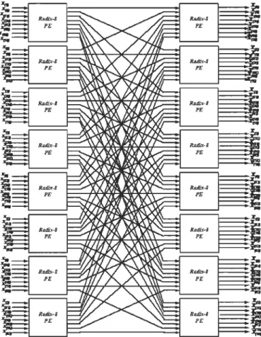
La clé conceptuelle du papillon modifié de la TRF à base r est la formulation de la TRF à radice-r comme r éléments de traitement élémentaires (BPE - Butterfly Processing Element) avec des structures identiques et un moyen systématique d'accéder les coefficients

multiplicateurs correspondants. Cela permet la conception d'un BPE avec le plus faible taux de multiplicateurs et d'additionneurs complexes, qui utilise r ou r - 1 multiplicateurs complexe en parallèle pour calculer chaque sortie du papillon conventionnel. Il y a une association simple entre les trois indices (TRF étape, papillon et élément) et les adresses des coefficients multiplicateurs nécessaires. Pour un environnement de processeur unique, ce type de BPE avec r multiplicateurs en parallèles entraînerait la diminution du délai du calcul de la TRF par un facteur de O(r). Un second aspect des papillons modifiés de la TRF à radice-r est, qu'ils sont également utiles dans les environnements du multitraitement en parallèle où cette structure en parallèle est réalisable au cours de chaque étage de la TRF. Si chaque BPE est exécuté sur le papillon modifié, cela signifie que chacun des r BPE en parallèles exécutera la même instruction simultanément, ce qui est très souhaitable pour la structure d'une seule instruction avec des données multiples (SIMD) sur certains des plus récentes cartes DSP.

En outre, on a développé un générateur d'adresses pour la TRF qui peut réduire la charge de calcul et l'accès aux mémoires en groupant les ensembles de données avec ses multiplicateurs correspondants. L'avantage de regrouper les ensembles de données avec ses correspondants multiplicateurs permettra de réduire les accès aux mémoires où lors de chaque étage la mémoire des coefficients est consulté l fois pour la procédure DIT et r(S-s) fois pour la procédure DIF où S = logrN - 1 et s

= 0, l , ..

, S - 1. En plus et à l'aide de ce concept, nous pourrions facilement prévoir l'apparition des multiplications triviales. La présence de la multiplication par ± 1 peut être facilement prédite pendant le processus de la TRF où en faisant donc, l'accès aux mémoires et les multiplications complexes pourraient être réduites ainsi que la multiplication par ± j peut être aussi prédite et qui peut être

incorporée dans les additions par la commutation des parties réelles et imaginaires des données. En plus de cela, la multiplication par

±"l{ ±j"l{

peut être prédite aussi où le nombre d'opérations arithmétiques peut être réduit de 6 à 2.

Dans ce domaine, nous avons développé également l'algorithme de la TRF à une seule itération qui est un outil utile pour détecter des fréquences spécifiques dans des signaux surveillés. Une des techniques les plus importantes dans l'analyse des caractéristiques d'un signal est l'extraction des informations utiles d'un signal surveillé. La surveillance des signaux est un domaine en expansion qui visent la détection des changements brusques pour une fréquence spécifique la détection d'un ensemble présélectionné de fréquences tel que RFID (Radio Frequency Identification) et dans le système de communication sans fil OF DM (Orthogonal Frequency Division Multiplex) dans lequel la TRF est un opérateur clé principal. Notre algorithme proposé a montré un gain significatif en vitesse et en rapport du signal au bruit quantifié (SQNR - Signal to Quantization Noise Ratio) en comparaison avec l'algorithme de Goertzel. Enfin, pour ce domaine nous avons développé le Low Complexity Input/output Pruning FFTs qui est une méthode utilisée pour calculer une DFT où un sous-ensemble des sorties sont nécessaires.

Abstract

Digital Signal Processing (DSP) is an engineering field that continues to extend its theoretical foundations and practical implications in the modem world from highly specialized aero spatial systems through industrial applications to consumer electronics. The Fast Fourier Transform is one of the most important topics in Digital Signal Processing that generates a map of a signal (called its spectrum) in terms of the energy amplitude over its various frequency components, at regular (e.g. discrete) time intervals, known as the signal's sampling rate. This signal spectrum can then be mathematically processed according to the requirements of a specific application (such as noise filtering, image enhancing, etc ... ). The quality of spectralînformation extracted from a signal relies on two major components: the first one is the spectral resolution which means a high sampling rate that will increase the implementation complexity to satisfy the time computation constraints. The second one is the spectral accuracy which is translated into an increasing of the data binary word-Iength that will increase normally with the number of arithmetic operations.

As a result, the FFTs are typically used to input large amounts of data; perform mathematical transformation on that data and then output the resulting data all at very high rates. The mathematical transformation IS executed by arithmetic operations (multiplications, summations or subtractions in complex values) following a specific dataflow structure that should control the systems' input/output. Multiplication and memory accesses are the most significant factors on which the execution time relies. The problem with the computation of an FFT with an increasing N is associated with the straightforward computational structure, the coefficient multiplier memories' accesses and

the number of multiplication that should be performed. In high resolution and better accuracy, this problem will be more and more significant for real time FFT implementation and in order to satisfy the time computation constraints. We should structure the input/output data flow that could reduce the coefficient multipliers accesses and also to reduce the computational load by targeting trivial multiplication. Memories' accesses are major concerns in implementation on DSP cards which on the most cases are costly in DSP cycles. Therefore, in a real time implementation, executing and controlling the data flow structure is important in order to achieve high performance that could be obtained by regrouping the data with its corresponding coefficient multiplier. By doing so, the access to the coefficient multiplier's memory will be reduced drastically and the multiplication by the coefficient multiplier wO will be taken out of the equation. In order to maintain lower arithmetic operations within the butterfly critical path (one complex multiplier and certain adders), we will be targeting hardware oriented Radix 2a or 4.8 which is an alternative way ofrepresenting higher radices by mean ofless complicated and simple butterflies.

In this thesis, we developed the self-sorting JMFFT (Jaber-Massicotte Fast Fourier Transform) algorithrn that cou Id benefit the trivial multiplication

±1,

±j

and

±F?{ ±jF?{

that will yield to the kernel core JMFFT's computation. One of the most significant impacts of the proposed structure from the hardware point ofview is that the coefficient's multiplier memory has been reduced from Nil to N18. The JMFFT was tested on the TMS320C6416 DSP platform using TI's Code Composer Studio which shows a significant gain in clock cycle reduction in comparison to the most recent published method 22 kernel core FFT. Furthermore, the JMFFT was benchmarked on the FFTW platform in which our proposed structure revealed a significant gain compared to

FFTW. The FFTW benchmark is an FFT bench platform assembled by Matteo Frigo and Steven G. Johnson at MIT (Massachusetts Institute of Technology). This platform compares the performance of different complex FFT implementations (40 FFT methods) based on speed and accuracy where performance is computed on a single processor environment. The FFTW platform includes an FFT method called FFTW _ESTIMA TE that outperforms ail other methods and is actually used in Matlab® software. Our results shown a speedup up to 30% compared to FFTW.

One of the most important techniques is the Signal-analysis/feature-extraction techniques which aim to extract useful information from a given monitored signal. Signal monitoring is an expanding domain that deals in detecting any abrupt changes for a special known frequency such as fault detection machine or to scan a pre-selected set of frequencies, as in radio-frequency identification (RFID) tags, the recognition of the dual-tone multi-frequency (DTMF), DNA analysis and in the orthogonal frequency division multiplex wireless communication (OFDM), wherein the Fast Fourier Transform (FFT) is a major key operator, particularly for cognitive radio. In this thesis, we developed the radix-r JM-Filter (Jaber Massicotte-Filter) which' is a combination of the radix-r one iteration FFT algorithm and the Goertzel's algorithm structures. Compared to Goertzel'~ filter, the proposed first and second order radix-r JM-Filter manifested a gain in the computational complexity reduction. The higher radix is; the highest gain is obtained.

Cellular and cordless phones rapidly became mass-market consumer products in which each wireless system has to combat transmission and propagation effects that are substantially more hostile than for a wired system. The advances in signal processing provided methods to overcome the anomalies of the mobile channel by accelerating the

growth of wireless communication and by tackling the channel problems by mean of the diversity reception concept that can substantially improve the link performance. Moreover, advanced digital modulation methods, such as spread spectrum or Multi-Carrier Modulation (MCM) appear suitable for wireless communication where Orthogonal Frequency Division Multiplexing (OFDM), a special form of MCM, will be used extensively in digital terrestrial broadcast systems, e.g. in DAB (Digital Audio Broadcasting) and DTTB. Theoretical aspects of the Pruning FFT (PFFT) have been thoroughly elaborated in past three decades and which was mainly concentrated on sequences that have Li consecutive non-zero input points at the beginning. In many applications, the percentage of required input/output bins is very small su ch as the 3GPP (The· 3rd Generation Partnership Project) LTE (Long Term Evolution) where the OFMDA's symbol size is 1024 in which 12 users equally share the available 600 sub-carriers. As a result only 50 of the 1024 FFT output bins (5%) are required for each mobile terminal. These partial input/output cases are important for the future wireless systems and because the PFFT can potentially achieve a significant speedup which is made it as a target by many applications such as cognitive radio. In this thesis, we have presented a novel JMIOPFFT (Jaber Massicotte Input/Output Pruning FFT) that shows an important gain in the computational complexity reduction compared to the most relevant published results.

Contents

Faible complexité et haute performance de la transformée de Fourier ... .ii

Dédicace ... iii Remerciements ... iv Résumé ...... v Abstract ...... viii Contents ...... xii List of Tables ... : ... xv

List of Figures ...... xix

Abreviations ...... xxvii

List of Symbols ... xxx

Chapter 1 Introduction ... 1

Chapter 2 The Radix-r Butterfly Processing Element ... 24

Paper 1: M. Jaber and D. Massicotte, "A New FFT Concept for Efficient VLSI Implementation: Part 1 Butterfly Processing Element", International Conference on Digital Signal Processing (DSP), Santorini, Greece, 5-7 July 2009 ... 27

Paper II: M. Jaber and D. Massicotte, "A New FFT Concept for Efficient VLSI Implementation: Part II - Parallel Pipelined Processing", International Conference on Digital Signal Processing (DSP), Santorini, Greece, 5-7 July 2009 ... 48 Paper III: M. Jaber, D. Massicotte, and Y. Achouri, "A Higher Radix FFT FPGA

Conference on Electronics, Circuits, and Systems (lCECS), Beirùt Lebanon, December 2011. ... 64 Chapter 3 A Novel Approach for the FFT Data Reordering ... 79 Paper IV: M. Jaber and D. Massicotte, "A Novel Approach for the FFT Data

Reordering", International Symposium on Circuits and Systems (lSCAS), Paris, May 2010 ... 81 Chapter 4 The JM-fiIter to Detect Specifie Frequencies in Monitored Signal.. ... 96 Paper V: M. Jaber and D. Massicotte, "The Radix-r One Stage FFT Kemel

Computation", International Conference on Acoustic, Speech, and Signal Processing (lCASSP), Las Vegas Nevada USA, April 2008 ... 98 Paper VI: M. Jaber and D. Massicotte, "Fast Method to Detect Specifie Frequencies

in Monitored Signal", International Symposium on Communications, Control and Signal Processing (lSCCSP), Cyprus, March 2010 ... 113 Paper VII: M. Jaber and D. Massicotte, The JM-filter to Detect Specifie Frequencies in Monitored Signal, to be submitted to a Journal after the end of the corifidentiality ...... : ... ; ... 131 Chapter 5 The JMFFT Core Kernel Computation ... 152 The JMFFT Core Kernel Computation ... 152 Paper VIII: M. Jaber and D. Massicotte, "The Self-Sorting JMFFT Algorithm

Eliminating Trivial Multiplication and Suitable for Embedded DSP Processor", accepted in NEWCAS, Montreal Canada, June 2012 ... 154

Paper IX: M. Jaber and D. Massicotte, "A Novel Radix-23 JMFFT Suitable for Embedded DSP Processor", ta be submitted ta a Journal after the end of the conjidentiality .................. 169 Chapter 6 Low Complexity Input/Output Pruning JMFFT Kernel Core ... 196 Paper X: M. Jaber and D. Massicotte, "Lowest Complexity Input/output Pruning

FFT", ta be submitted ta a Journal after the end of the conjidentiality ... 198 Chapter 7 Conclusion and Future Works ... 220 References .... 225

List afTables

Chapter 1

Table 1: Number of non-trivial real multiplications for various FFTs ... ... ... 15 Table 2: Number of non-trivial real additions for various FFTs ... ... ... ... ... ... 16 Chapter 2

Paper 1: A New FFT Concept for Efficient VLSI Implementation: Part I-Butterfly Processing Element; DSP'09, Santorini, Greece, 5-7 July 2009

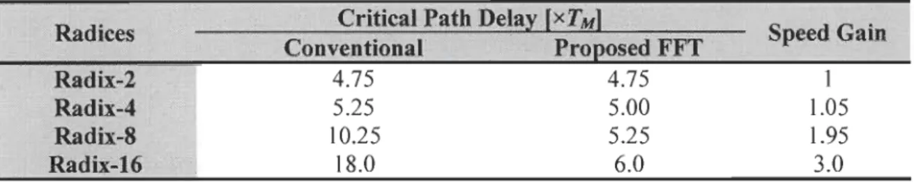
Table 1: Critical path delay of BPE for convention al and proposed BPE with Radix-2,4,8 and 16 in order to obtain the first outputs... 42 Table 2: Time computation results in terms of TM between the proposed structures

and the conventional one and the speed gain comparison with Cooley-Tukey'

(radix-2) for N

=

4096

..

.

...

...

....

...

..

.

...

...

..

.

...

.

..

...

.

...

..

...

42

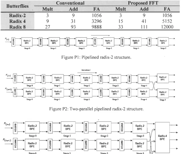
Table 3: Number of real multiplications and additions for BPE and in term of FA

(multiplier on 16-bit and adder on 32-bit)... 44 Paper II: A New FFT Concept for Efficient VLSI Implementation: Part II Parallel

Pipelined Processing; DSP'09, Santorini, Greece, 5-7 July 2009

Table 1: Critical path delay of BPE for conventional and proposed BPE with Radix-2,4,8 and 16 in order to obtain the first r outputs... 56 Table 2: Number of real multiplications and additions for BPE and in term of FA

(multiplier on 16-bit and adder on 32-bit)... ... 58 Table 3: Area and computation time of the· proposed multistage parallel pipelined

FFT architectures as shown in Fig. PI-P6... ... 61 Paper III: A Higher Radix FFT FPGA Implementation Suitablefor OFDM Systems

ISCASS 2011, Beirut Lebanon

Table 1: Cost Evaluation in MS/s/Slice for an FFT of size 4096... 76 Table 2: Latency time for an FFT of size 4096 (in

IlS)...

...

...

...

....

...

...

76 Table 3: Computational Time of the FFT execution for a size 4096(in

Il

S)..

....

....

...

77 Table 4: Number of embedded multiplier used for devices and methods... 77 Chapter 3

Paper IV: A Novel Approach for the FFT Data Reordering, Int. Symp. On Circuit and System (ISCAS), Paris, May 2010

Table 1: Memory for table index number... ... 92 Chapter 4

Paper V: The Radix-r One Stage FFT Kernel Computation, ICASSP 2008, April First Las Vegas Nevada USA

Table 1: Number of cycles need to execute a 4096-points FFT for different radices by factoring the adder matrix... 110 Table 2: Number of cycles needs to execute a 4096-points FFT for different radices

by implementing r BPEs in parallel (Fig. 2) ... 110 Table 3: Number of cycles needs to execute a 4096-points FFT for different radices

by using r OSPE (Fig. 4)... ... ... ... ... ... ... ... ... ... ... 110 Paper VI: Fast Method to Detect Specifie Frequencies in Monitored Signal,

International Symposium on Communications, Control and Signal Processing (ISCCSP 2010), Cyprus, March 2010

Table 1: Performance of adder tree structures for r-input (Fig. 9)... .... 126 Table 2: Hardware resources in term of real adders (Adder) and multipliers (Mult) to

implement the different BPEs in our study... 128

Paper VII: The JM-filter. to Detect Specifie Frequencies in Monitored Signal, to be

submitted to a Journal after the end of the confidentiality

Table 1: Computational Complexity in terms of real arithmetic operation of the proposed first order radix-2/4 JM-filters and first order Goertzel filter for different sizes of

N

..

..

...

...

...

...

..

.

.. .

..

....

.

.

.

...

..

...

145 Table 2: Computational complexity in terms of real arithmetic operation of the

proposed SECOND order radix-2/4 JM-Filters and second order Goertzel filter for different sizes of complex input N... ... 145 Chapter 5

Paper VIII:

Table 1: Table 2: Table 3: Table 4: Table 5:

The Self-Sorting JMFFT Algorithm That Eliminates Trivial

Multiplication Which is Suitable for Embedded DSP Processor,

submitted to NEWCAS

2012,

Montreal Canada

Comparison in terms of memory accesses to the coefficient multiplier in [5] versus the proposed one where each complex access is counted as1 ... ; ... 161 Comparison in terms of real multiplication between the cited methods in [5] versus the proposed one ... 162 Comparison in terms of real addition between the cited methods in [5] versus the proposed one... 162 Comparative results in term of clock cycle of the cited methods versus the proposed method for different FFT sizes... ... 164 Comparison of the coefficients multiplier's memory requirement of

Paper IX: Table 1: Table 2: Table 3: Table 4: Table 5:

the cited methods versus the proposed method where the size is computed in term ofbyte ... 165

A Novel Radix-23 JMFFT Suitable for Embedded DSP Processor, to be submitted to a Journal after the end of the confldentiality

Comparison in terms of real multiplication between the cited methods in [8] versus the proposed one ... 190

Comparison in terms of real addition between the cited methods in [8] versus the proposed one... .... ... ... ... .... ... ... ... 190 Memory accesses count to the coefficient multiplier where each complex access is counted as

1...

191 Comparative results in term of clock cycle of the cited methods versus the proposed method for different FFT sizes... ... ... ... ... ... 192

Comparison of the coefficients multiplier's memory requirement of the cited methods versus the proposed method where the size is computed in term ofbyte ... 192

List of Figures

Chapter 1

Figure 1: The FFT decomposition: An N point signal is decomposed into N signais each containing a single point. Each stage uses an interlace decomposition,

separating the even and odd numbered samples... 5

Figure 2: Three stages in the computation of an N = 8-point DIT DFT... 7

Figure 3: Three stages eight-point DIF FFT algorithm... ... ... 7

Figure 4: Eight-point DIF FFT Signal Flow Graph (SFG).. ... ... 9

Figure 5: Basic butterfly computation for the DIF FFT algorithm... 9

Figure 6: Basic butterfly computation in a radix-4 FFT algorithm... ... ... ... ... .... 10

Figure 7: 12 point PFA (NI =4, N2 =3)... 13

Figure 8: Butterfly for SRFFT algorithm ... ,... 14

Chapter 2 Paper 1: Figure 1: Figure 2: Figure 3: Figure 4: Figure 5: A New FFT Concept for Efficient VLSI Implementation: Part 1-Butterfly Processing Element; DSP'09, Santorini, Greece, 5-7 July 2009 SFG of the a) radix-4 and b) radix-8 butterflies [2] ... .. Radix-r partial BPE (llh output) (a) using Br in Eg. (16), and the symbol 36

b)...

..

...

..

...

...

...

39

Maximize the data throughput using r BPE in parallel... 39

SFG of the proposed radix-4 BPE and the value of the multipliers

U

with i=1, .. ,5... ... ... ... ... ... ... ... ... ... ... ... ... ... ... ... ... ... 40

SFG of the proposed radix-8 BPE and the value of the multipliers

U

With i =1,2, ... ,11... ... ... 40

Figure 6: Figure 7:

S Stages Radix-r Pipelined FFI... 42

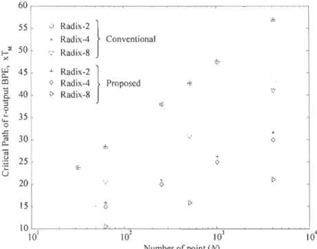
Critical path delay for r-output pipeline FFI conventional and proposed FFI Radix-2, 4 and 8... 44

Paper II: A New FFT Concept for Efficient VLSI Implementation: Part 11-Parallel Pipelined Processing; DSP'09, Santorini, Greece, 5-7 July 2009 Figure 1: Figure 2: Figure 3: Figure 4: Figure 5: S Stages Radix-r Pipelined FFI... ... ... ... ... ... ... ... 53

r-parallel pipelined radix-r for lBPE structure... 54

Iwo parallels radix-2 pipelined BPEs connected to two radix-4 BPEs... 55

SFG of the proposed radix-4 BPE and the value of the multipliers M; with i=I, .. ,5... ... ... ... ... ... ... ... ... .... ... ... ... ... .... ... 56

SFG of the proposed radix-8 BPE and the value of the multipliers M; With i =1,2, ... ,11... ... ... ... ... ... ... ... ... ... ... ... ... ... ... .... 57

Figure Pl: Pipelined radix-2 structure... 58

Figure P2: Iwo-parallel pipelined radix-2 structure... ... 58

Figure P3: Four-parallel pipelined radix-2 structure... 58

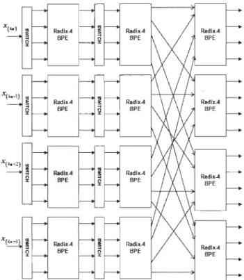
Figure P4: Four-parallel pipelined radix-4 structure ... :... 59

Figure P5: Eight-parallel pipelined radix-2 structure... 59

Figure P6: Eight-parallel pipelined radix-8 structure... 60

Paper III: A Higher Radix FFT FPGA Implementation Suitable for OFDM Systems ISCASS 2011, Beirut Lebanon Figure 1: SFG of the radix-8 DIT butterflies [3] where the highlighted red portion represents the butterfly critical path used in FFI conventional... 69 Figure 2: SFG of the proposed radix-8 BPE and the value of the multipliers M; are

Figure 3: Figure 4: Figure 5: Figure 6: Figure 7: Chapter 3

defined in [2] where the highlighted red portion represents the butterfly critical path (named BPE JFFT)... ... ... ... ... ... ... ... ... ... 71 Pipelined FFT structures: a) Radix-2 SDF structure (R2SDF) for N = 16,

b) Radix-4 SDC structure (R4SDC), and c) Radix-2 MDC structure

(R2MDC)... 72 Fixed-point simulation with QPSK signais ... . Scenario 1: SQNR comparison for coefficients' word-Iength 6 to 9-bit and input/output data's word-Iength is fixed to 16-bit where

72

N=4096... 73 Scenario 2: SQNR comparison for input/output data's word-Iength 8 to 24-bit

and coefficients' word-Iength is fixed to 8-bit where

N=4096... 74 Complex Multiplier case studied: a) Case 0, b) Case 1, c) Case 2, and d) Case

3 ... 75

Paper IV: A Novel Approach for the FFT Data Reordering, Int. Symp. On Circuit and System (ISCAS), Paris, May 2010

Figure 1: Figure 2:

Figure 3:

Chapter 4

C Function of the proposed method... . . .. 88 Performance gain of proposed method compared to Rius & de Porrata-Doria [8], in solid line, and Pei & Chang [10], in dash line, for radix-2... ... 90 FFTW benchmark results of the proposed method (JFFT) compared to

Paper V:

Figure 1: Figure 2: Figure 3: Figure 4:

The Radix-r One Stage FFT Kernel Computation, ICASSP 2008, April First Las Vegas Nevada USA

BPE for the FFT Radix-r (a) using Br in (11) and the symbol (b)... 104 Maximize the data throughput using r BPEs in parallel... 104 Radix-r OSPE (a) using (26) and the symbol (b)... .... ... ... ... ... 109 Maximize the data throughput using r OSPE in parallel... 109 Paper VI: Fast Method to Detect Specifie Frequencies in Monitored Signal,

International Symposium on Communications, Control and Signal Processing (ISCCSP 2010), Cyprus, March 2010

Figure 1: The L TI filter represented by Eq. (1)... ... .... 117 Figure 2: Figure 3: Figure 4: Figure 5: Figure 6: Figure 7: Figure 8: Figure 9:

Representation of the L TI filter by its z transform. . . 117 The first-order Goertzel... ... ... 117 The second-order Goertzel filter... 118 C Function of the Goertzel' s algorithm [5]... 118 Radix-r one iteration FFT using r consecutive complex multipliers (a) and one complex multiplier (b)... ... ... ... ... ... ... ... ... ... .... 121 SFG of the radix-4 (a) and radix-8 (b) BPE from Fig. 5... 122 Parallel Implementation of Goertzel' algorithm... ... ... ... ... ... ... ... 122 Pipelined complex multiplier using 4 real multipliers (a) and three real multipliers (b)... ... ... ... ... ... ... ... ... ... ... ... ... ... ... ... 125 Figure 10: Adder tree circuit structures a, and b... 125 Figure Il: Speed gain of proposed one iteration compared to Goertzel's algorithm using

Eg. (15)... ... ... ... .... ... ... ... ... ... ... ... ... ... 127

Paper VII: The JM-filter to Detect Specifie Frequencies in Monitored Signal, to be submitted to a Journal the end of the confidentiality

Figure 1: The LTI filter represented by Eg. (1)... 134 Figure 2: Representation of the L TI filter by its z transforrn... 134 Figure 3: The first-order Goertzel... ... 134 Figure 4: The second-order Goertzel filter... ... 135 Figure 5: C Function of the Goertzel's algorithm [5]... ... 136 Figure 6: Radix-r one iteration JMFFT using r consecutive complex multipliers (a) and

one C-MAC (b)... ... ... ... ... ... ... ... ... ... ... ... ... ... ... 138 Figure 7: Parallel Implementation of Goertzel' algorithm... 139 Figure 8: The radix-r first order JM-filter... .... ... ... ... ... ... ... ... ... ... 140 Figure 9: The radix-r second order JM-filter... ... ... ... ... .... ... ... ... ... ... 140 Figure 10: The radix-2 first order JM-filter... 141 Figure Il: The radix-2 second order JM-filter... 142 Figure 12: The radix-4 first order JM-filter... ... .... ... ... ... ... ... ... 143 Figure 13: The radix-4 second order JM-filter... ... 143 Figure 14: SQNR Comparison between the cited method in [16] with a scaling factor 11

N and the cited method in [17] with a scaling factor 1t I( 4N) where the data and twiddle factor are guantized to 16 bits width ... ... .... ... ... 146 Figure 15: SQNR Comparison between the proposed first order radix-2/4 and the first

order Goertzel's algorithm on a data and twiddle factor of 16 bits width where the Scaling factor for ail method is 1IN. ... ...... 147

Figure 16: Difference in SQNR between the proposed first order radix-2/4 and the first order Goertzel's algorithm on a data and twiddle factor of 16 bits width the Scaling factor for ail method is liN.. ..... ... ... ... 147 Figure 17: SQNR Comparison between the proposed first order radix-2/4 and the first

order Goertzel's algorithm on a data of 24 bits width and twiddle factor of 16 bits width where the Scaling factor for ail method is 1/N............... ...... 148 Figure 20: Difference in SQNR between the proposed first order radix-2/4 and the first

order Goertzel's algorithm on a data of 24 bits width and twiddle factor of 16 bits width where the Scaling factor for ail method is lIN... 148 Chapter 5

Paper VIII: The Self-Sorting JMFFT Algorithm That Eliminating Trivial Multiplication And Suitable for Embedded DSP Processor, submitted to NEWCAS 2012, Montreal Canada

Figure 1: Computing two butterflies together in one stage of the radix-2 DIF FFT diagram [5] where m is given in equation (16)... ... ... ... ... ... 161 Figure 2: Comparison of c\ock cycle reduction between our proposed method and the

Referenced methods (TI and Cited)... ... ... ... ... ... ... .... 164 Figure3: FFTW benchmark results of the proposed method for the radix 4... ... 165 Figure 4: FFTW benchmark results of our previous method (JFFT) for the radix-4

[71]... 166 Paper IX: A Novel Radix-~ JMFFT Suitable for Embedded DSP Processor, to be

submitted to a Journal the end of the confidentiality

Figure 2: Figure 3: Figure 4: Figure 5: Figure 6: Figure 7: Figure 8:· Figure 9: Figure 10:

each containing a single point. Each stage uses an interlace decomposition, separating the ev en and odd numbered samples... ... 172 Three stages in the computation of an N

=

8-point DIT DFT... ... ... ... ... .... 173 Basic butterfly computation for the DIT FFT algorithm... 174 Eight-point DIT FFT Signal Flow Graph (SFG)... ... 175 Three stages eight-point DIF FFT algorithm... 175 Basic butterfly computation for the DIF FFT algorithm... ... 176 Eight-point DIF FFT Signal Flow Graph (SFG)... 176 Radix-8 DIT butterflies where the highlighted red portion represents the butterfly critical path... 177 Signal flow graph (SFG) of 8 points DIT FFT on the proposed structure... 183 8th root of unit y . . . .. 186 Figure Il: The proposed JMFFT 23 butterfly structure for trivial computation where the

inputs/outputs are provided by equation (32)... ... ... ... 188 Figure 12: The proposed JMFFT 23 butterfly structure for non-trivial computation.... 188 Figure 13: Reference methods, TI and REF, c10ck cycle reduction compared with our

proposed method... 191

Chapter 6

Paper IX: Low Complexity Input/output Pruning JMFFTs Suitablefor the OFDMA's

3GPP LTE Implementation, to be submitted to a Journal the end of the confidentiality

Figure 2: Figure 3: Figure 4: Figure 5: Figure 6: the reference [13]... 207 Number of operations required by the one cited in reference [13] in direct implementation and our proposed method for N=8192 and Li = 8192, 307 and33... ... ... ... ... ... ... ... ... ... ... ... ... ... ... ... 212 Operation's reduction ratio between the proposed and the cited method in a) and b) is the zoomed version of figure a)... ... ... .... ... ... ... ... ... ... 213 Precision based on SQNR, a) without 2BF filtering and b) by using the 2 BF filtering... ... 214 Comparison among the proposed and the cited pruned FFTs for N = 1024

and Li = Lo = 1024... ... ... ... ... ... ... ... ... ... ... ... 215 Operation's reduction ratio between the proposed and the cited method by using 2 BF method when Li = Lo and N = 1024... ... 215

AG BPE Cag CAGDIF CAGDIT C-MAC DFT DIF DIT DNA DTMF FA FFT FFTW IPJMFFT JMIOPFFT JM JMFFT LTE MAC MDC

Abreviations

Address Generator

Butterfly Processing Element Coefficient Address Generator

Coefficient Address Generator for the DIF FFT Coefficient Address Generator for the DIT FFT Complex multiply-accumulator

Discrete Fourier Transform Decimation In Frequency Decimation In Time Deoxyribonucleic Acid Dual-tone multi-frequency Full adder

Fast Fourier Transform

Fast Fourier Transform in the West Input Pruning JMFFT

JM Input Output Pruning FFT Jaber Massicotte

Jaber Massicotte FFT Long Term Evolution Multiply-accumulator

MIMO-OFDM OFDM OFDMA 0100 OSPE pdf PFFT RAG RAGDIF RAGDIT RCAG RDAG RFID SDC SDF SFG SQNR TDF TDSN TRF VLIW VLSI

Multiple Input Multiple Output - Orthogonal Frequency Division Multiplexing

Orthogonal Frequency Divisions Multiplex

Orthogonal Frequency Division Multiplexing Access Ordered Input Ordered Output

One Stage Processing Element Probability density function Pruning FFT

Reading Address Generators

Reading Address Generators for the DIF FFT Reading Address Generators for the DIT FFT

Reading Coefficients (twiddle factors) Address Generator Reading Data Address Generator

Radio Frequency IDentification Single-path Delay Commutator Single-path Delay Feedback structure Signal flow graph

Signal to Quantization Noise Ratio La Transformée Discrète de Fourier Traitement Du Signal Numérique La Transformée Rapide de Fourier Very Long Instruction Word Very Large Scale Integration

WAG

WDAG

WFTA

3GPP

Writing Address Generator

The writing data address generator

Winograd Fourier Transform Algorithm

x[n] N nk -}(21</ N)nk W_N =e ·2 )

*

(a,r,fJ)

List ofSymbols

the input sequence

the output sequence the transform length

The twiddle factor in butterfly structure The complex number

=

-}

The butterfly matrix The adder tree matrix The twiddle factor matrix The integer part operator of x The operation x modulo N

Résumé

du

Chapitre 1

Dans ce chapitre, nous présentons la transformée discrète de Fourier (TDF) et la transformée rapide de Fourier (TRF). La Transformée Rapide de Fourier est simplement une TDF calculée selon un algorithme permettant de réduire le nombre d'opérations et, en particulier, le nombre de multiplications à effectuer. Une brève description de la dérivation de la transformée rapide de Fourier sera présentée en mettant l'accent sur les deux versions de l'algorithme, avec

«

entrelacement temporel » et avec

«

entrelacement fréquentiel ». Par la suite, on présentera une brève description du défi pour réduire la complexité de l'algorithme. Une de notre contribution majeure dans ce domaine, est la réduction de la complexité du passage critique du papillon à radice-r. Pour améliorer de manière significative la rapidité de ce traitement, on a suggéré un générateur d'adresses pour la transformée rapide de Fourier dont le but est d'effectuer toutes les opérations de réarrangement des données entrées/sorties. Ce générateur d'adresses nous a permis de regrouper les données avec les coefficients multiplicateurs correspondants tout en prédisant

l'apparition des multiplications triviales (8th root of unit y). De plus, dans cette thèse on a abordé le sujet de la détection d'une fréquence spécifique tout en proposant un filtre, nommé JM-Filter avec une complexité réduite en comparaison avec celle de Goertzel. Dans de nombreuses applications telles que le Long Term Evolution (L TE) et la radio cognitive, qui est basée sur l'Orthogonal Frequency Division Multiplexing OFDM, on aura besoin de calculer un certains nombres de sorties de la TRF où on a appliqué de manière efficace des zéros sur les entrées. Notre contribution dans ce sujet est basée sur l'introduction d'un

algorithme qui peut réduire la complexité du calcul en se comparant avec les méthodes les plus récemment proposées.

Introduction

Digital Signal Processing (DSP) is an engineering field that continues to extend its theoretical foundations and practical implications in the modem world from highly specialized military systems through industrial applications to consumer electronics. One of the most exciting aspects of DSP use is in new applications such as DNA that are impossible to implement using analog technology where a digital signal processor may be called on to perform one or more of several functions involving algorithmic processing of the digitized signaIs. So, digital signal processing is one of the most powerful technologies that will shape science and engineering in the upcoming centuries.

For the last decade, the DFT and ail resulting algorithms known collectively as Fast Fourier Transform (FFT) showed a great interest for their applications in which revolutionary changes have already been made in a broad range of fields su ch as: Speech compression [1], Digital filters [2], Image processing [3], Radar [4], OFDM (Orthogonal Frequency Divisions Multiplexing) [5]- [8], Wireless communications [9]-[11], DNA analysis and a lot of other non-cited domains. Therefore, the Discrete Fourier Transform (DFT) is the decomposition of a sampled signal in terms of sinusoidal (complex

exponential) components expressed as: N-I

X(k)

=

LX(n)w; , kE

[O,N-1]

(1),

n=O

and because of its computational requirements, the DFT algorithm usually is not used for real time signal processing. For the last decencies, the main concem of the researchers was

to develop an FFT algorithm in which the number of operations required is minimized. Since Cooley and Tukey presented their approach showing that the number of

· may be considerably reduced by using one of the fast Fourier transform (FFT) algorithms. The basis of the radix-2 FFT is that a DFT can be divided into two smaller DFTs, each of which is divided into two smaller DFTs, and so on, resulting in a combination oftwo points DFTs kemel. Cooley and Tukey's method, which is known as fast algorithms for DFT computation, is based on the divide-and-conquer approach that was introduced by

Danielson and Lanczos in 1942 as shown in Figure 1 [12]. The advantage of appropriately

breaking the DFT in terms of its partial DFTs is that the number of multiplications and the number of stages may be controlled. The number of stages often corresponds to the amount of global communication and/or memory accesses in implementation, and thus, reduction in the number of stages is beneficial. Several efficient methods are used repeatedly to split the DFTs into smaller (two or four-point) core calculations, where the symmetry and periodicity properties of the DFT are exploited to significantly lower its computational requirements. 1 Signal of 16 points 2 SignaIs of 8 points 4 SignaIs of 4 points 8 SignaIs of 2 points 16 SignaIs of 1 point 0123456789101112131415

Figure 1: The FFT decomposition. N point signal is decomposed into N signais each containing a single point. Each stage uses an interlace decomposition, separating the even and odd numbered sampi es.

2. Derivation of the FFT

The computational complexity of the DFT increases as the square of the transform length, and thus, becomes expensive for large N. The fast Fourier transform (FFT) provides

an effective tool for the calculation of Fourier transforms that is based on the divide-and-conquer approach. In the FFT case, the input data x(n) are divided into subsets on which the

DFT is computed. Then the DFT of the initial data is reconstructed from these intermediate results. Ifthis strategy is applied recursively to the intermediate DFTs, an FFT algorithm is

obtained. Sorne ofthese methods are:

w Common Factor Aigorithms (decimation-in-time (DIT) or Cooley-Tukey FFT algorithm [13] and decimation-in-frequency (DIF) or Sande-Tukey

FFT algorithm [14]),

w Prime Factor Aigorithm (PFA) [15], W Mixed Radix Aigorithm (MRA) [15],

W Winograd Fourier Transform Aigorithm (WFTA) [16] and

W Split-Radix Aigorithm (SRA) [17]. 2.1 Common Factor Aigorithms

In the common factor algorithms, the transform length N, is decomposed into arbitrary

factors (N

=

rl, r2, ... , rk) and if ail the factors, rj, are equal, the algorithm is called radix-r algorithm. Two different versions of the algorithm that are dual of each other, which are

always derived depending on how the decimation is performed. The two versions have the

same computational complexity and are called decimation-in-time (DIT or Cooley-Tukey)

. "

2.1.1 The DIT and DIF Aigorithms

In mid-1960s, J.W. Cooley and J.W. Tukey proposed their first algorithm known as

decimation-in-time (DIT) or Cooley-Tukey FFT algorithm, which first rearranges the

input elements into bit-reverse order, then builds up the output transform in log2 N

iterations figure (2) [12], [13] and [18].

X(O) 2-point X(4) _DFT X(2) 2-point X(6) _DFT X(I) 2-point X(5) _DFT X(3) 2-point X(7) _DFT Combine 2-point DFT's Combine 2-point DFT's X(O) X(I) X(2) Combine X(3) 4-point X(4) DFT's X(5) X(6) X(7)

_ Figure 2: Three stages in the computation of an N = 8-point DIT DFT.

It is also possible to derive FFT algorithms that first go through a set of log2 N iterations

on the input data, and rearrange the output values into bit-reverse order. These are called

decimation-in-frequency (DIF) or Sande-Tukey FFT algorithm Figure (3) [19].

X(7) -1 1 Wg 3 w8 Combination 4-I)Onl DIT Combination 4-pont DIT

2.1.2 The Radix-2 Aigorithm

In this section, the development of the radix-2 DIF FFT will be described in detail. The integers n and k in equation (1) (for the case N

=

2Y) can be expressed in binary numbers as

[15],

- 2y_-1 ₂y_-2

n - nY-1

+

ny-2

+

... +

no (2),

k - 2y-1 L- 2y_{-2 L-}

_ka

- ""(-1

+

""(-2

+ ... +

(3).

in which n and k can take the values 0 and one only. Equation (1) can be rewritten as

(4)

Now, the

fi

e

sum can be divided into y separate summations

(5)

(6)

(7)

The computation of equation (1) has been divided into IOg2N

=

Y stages, each having a computational complexity of N, and thus, the result of the manipulations is that the total computational complexity has decreased from N2 to N IOg2 N. If the result needs to be in the natural order, an unscrambling stage for Xy is needed:

The signal flow graph for an 8-points radix-2 DIF FFT is shown in figure (4) in which the butterfly has been introduced as the primitive operation of the FFT. The radix-2 butterfly consists oftwo complex additions and one complex multiplication and it is shown in figure (5).

Figure 4: Eight-point DIF FFT Signal Flow Graph (SFG).

a -~~---.(

b_~O--_ _ _ ~

Figure 5: Basic butterfly computation for the DIF FFT algorithm.

2.1.3 Higher Radix

Another class of FFTs subdivides the initial data of length N not aIl the way down to the trivial transform of length 2, but rather only down to sorne other smalt power of two, four or eight (Figure 6). The result obtained in the above section could be extended to any base r that can be developed using the same techniques as for radix-2 case.

(8)

(9) The derivation of such algorithm will not be discussed, but sorne key points are listed below.

• Transform length N

=

r"'

where m is an integer.

• The arithmetic complexity is N x logrN x the arithmetic complexity of the radix

r butterfly.

• The number of stages is equal to logrN.

• The number of butterflies in each stage is equal'to Nlr.

• Each butterfly has r-inputs and r-outputs and r - 1 twiddle factor multiplication.

The advantage of using higher radix is that the number of multiplications and the number of stages decrease. The number of stages often corresponds to the amount of global communication and/or memory accesses in an implementation, and thus, the reduction in the number of stages is beneficial if communication is expensive as is the case in most hardware implementation [15], [20] and [21]. Up to date, the most disadvantage ofusing a higher radix is that the butterfly becomes more complicated and can be difficult to implement. Most subsequent authors have directed their attention to the special case of N

=

2m due to its simplicity in programing and the restricted choice of values of N is adequate for a majority of applications.

wJ'

(.) lb)

2.2 The Mixed radix and Prime Factor Aigorithm (PF A)

There are, however, sorne applications in which a wider choice of values of N is needed,

especially in speech's spectral analysis and economic series data. Since the transforrn

length is a problem, the mixed radix approach makes it possible [22]-[23]. This approach

was achieved by decomposing the matrix Tr into a radix-3 stage and a radix-5 stage in

order to compute a 15 points DFT [12].

Gentleman and Sand have extended the development of the general case by mentioning

the existence of a mixed radix FFT program written by sand [14]. So, R. C. Singleton

proposed an improved method by decomposing N into its prime factor, yielding an

algorithm for computing the mixed radix Fast Fourier Transform [21]. The larger the prime

factor of N is the worse this methods works because if N is prime, then no subdivision is

possible, and the complexity would be of order N2•

Since the twiddle factors dominate the arithmetic workload in the corn mon factor

algorithm, it seems logical to try to remove them and that is exactly what prime factor

algorithms are ail about. This approach can only be used if N can be decomposed into

factors relatively prime, i.e.

(10).

Therefore, the greatest common divisor for NI and N2 is equal to one and for this case, n

and k can be expressed as [15],

(11),

k

=

[N

2

[N

;

'

]t

,

x

lG

+[

N,

[N,

-

'

]t

2

X

k

₂ (12)

where

[X]

N

denotes

x

modulo N and

[x

-

I

L

denotes the multiplicative inverse of

x

reduced moduloN.

Using these expressions equation (1) can be represented as

dimensional transform without inverting the twiddle factor. The signal flow graph of a 12 point prime factor algorithm is shown in figure (7) for NI = 4 and N2 = 3.

These are essentially three drawbacks of the prime factor algorithm:

• Since N to be decomposed into factors that are relatively primes, these factors will be large if N is large. This means that the short-Iength DFTs, which have a length, equal to these factors, becomes expensive to implement.

• There are more severe restrictions on the transform length than in the case of the corn mon factor algorithm.

These problems were dealt with and developed for the first time by S. Winograd and were referred as the Winograd Fourier Transform Aigorithm (WFTA) [16]. Winograd used the indexing scheme from the prime factor algorithm, expressed in small DFTs in terms of convolution, and combined this with efficient methods for computing periodic convolution [24]. The price paid for this decrease in multiplication compared to common factor algorithms, is a significant increase in the number of addition and the irregular structure [24].

X(O) 3-Poiot }O)

'

1

3₎ 4-Poiot DFT DFT i,4) X(6 (8) (9) 3-Poiot

~

'1

4) 4-Poiot DFT )il) (7) (5) ~10 DFT (1) 3-Poiot X(6) X(8) DFT 'f0) ₍₂₎ X(1 4-Poiot

1

2) DFT (5 _3-Poiot

~!

DFT (7) (11)

Figure 7: 12 point PF A (NI =4, N2 =3).

2.3 Winograd Aigorithm (W A).

Winograd algorithms are in sorne way analogous to the base-4 and base-8 FFTs, where he has derived a highly optimized coding for taking small-N discrete Fourier transforms. The method involves a reordering of the data both before the hierarchical processing and after it, but it allows a significant reduction in number of multiplication in the algorithm. For sorne especially favorable values of N, the Winograd algorithm can be significantly (up to factor 2) faster than the simple FFT algorithms, however, this advantage must be weighed against the considerably more complicated data indexing involved in these transforms. So, in 1977 based on Winograd method, Silverman proposed an improved method to calculate the FFT [25].

2.4 The Split Radix Aigorithm (SRA)

The split radix algorithm is an FFT based algorithm which was introduced by R. Yavne [26] and then developed by Duhamel and Hollmann [17]. It seems that the split·radix has achieved the lowest published arithmetic operation count (total exact number of required real additions and multiplications) on a data of size N which is a power of two [27]-[32]. The basic idea behind the SRFFT as derived by Duhamel and Hollman [17] is the

application of a radix 2-index map to the even-indexed terms and a radix-4 map to the odd-indexed terms. Under these indexing scheme equation 1 can be rewritten as

N

X(,,)

~

~(x(") +X

H:)

Jw

~

"

'

(14)

for the even index terms, and

N

X(".,)

=

~((

x(.)

-X

(

"

4)

J-

+

(

"

7)

-X("

,d

Jw

~

w

~

'

(15)

(16)

for the odd index terms. This results in an "L-shaped butterfly" figure (8), which relates a

length N DFT to one length N/2 DFT and two-length N/4 DFT [33]. Such algorithms are known by having the lowest of both multiplication and addition for length 2m FFTs, but it involves significantly more butterfly computations than radix 4 Cooley-Tukey Algorithms

[34], [52] and [58].

x(n) ~----'?

A 8

Figure 8: Butterfly for SRFFT algorithrn.

Use for

X(4k+ 1)

Use for X(4k + 3)

In the previous sub sections, different algorithm and butterfly structures for the dedicated FFT were cited. The main objective of these proposaIs was a reduction in computation and particularly the reduction in the number of multiplications where the most common way to compare algorithms is based on the number of arithmetic operations.

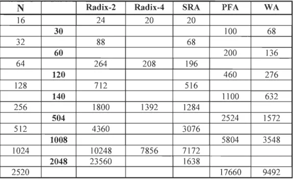
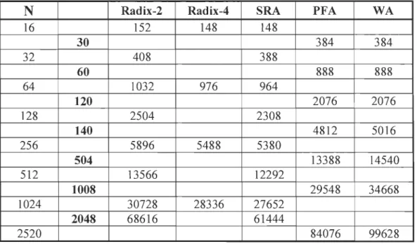
In Table 1 and Table 2 the number of real multiplications and real additions required for different algorithms are listed [15] and [35]. In these tables; it is assumed that non-trivial complex multiplication is implemented using 3 real multiplications and 3 real additions. It is clear that the split radix and the Winograd algorithms offer the lowest number of multiplications for small and medium length FFTs whereas the Winograd algorithm require less multiplications than every other algorithm for long FFTs. From Table 2, it can be seen that the split radix algorithm offers the lowest number of additions.

Table 1: Number of non-trivial real multiplications for various FFTs

N

Radix-2

Radix-4

SRA PFA WA

16 24 20 20

30

100 68 32 88 68

60

200 136 64 264 208 196

120

460 276 128 712 516

140

1100 632 256 1800 1392 1284

504

2524 1572 512 4360 3076

1008

5804 3548 1024 10248 7856 7172

2048

23560 1638 2520 17660 9492

In conclusion it is hard to make a fair and general comparison between the different algorithms betause the importance of different properties of the algorithms is depending on the implementation. In the case of hardware implementation of FFT processors there are

number of other algorithm's properties that should be dealt with such as: regularity,

modularity, parallelism and simplicity which are mostly offered by the common and prime factor algorithms.

Table 2: Number of non-trivial real additions for various FFTs

N

Radix-2

Radix-4

SRA PFA WA

16

152

148

148

30

384

384

32

408

388

60

888

888

64

1032

976

964

120

2076

2076

128

2504

2308

140

4812

5016

256

5896

5488

5380

504

13388

14540

512

13566

12292

1008

29548

34668

1024

30728

28336

27652

2048

68616

61444

2520

84076

99628

Finally, in this chapter we will define the problematic and major challenges, to

finally demonstrate c1early our methodology, originality and scientific contribution.

3.

Problematic and major challenges

The FFTs are typically used to input large amounts of data; perform mathematical

transformation on that data and then output ail the resulting data at very high rates. The

mathematical transformation is translated into arithmetic operations (multiplications,

summations or subtractions in complex values) following a specifie dataflow structure that

should control the systems' input/output. Multiplication and memory accesses are the most

significant factors on which the execution time relies therefore; the major challenge is to

reduce the multiplication load in a simple dataflow structure to facilitate the parallel and

pipeline implementation in one hand and on the other hand to reduce the coefficient multiplier memories' accesses by regrouping the data with its corresponding coefficient multiplier. The quality of spectral information extracted from a signal relies on two major components:

• Spectral resolution which means high sampling rate that will mcrease the implementation complexity to satisfy the time computation constraints .

• Spectral accuracy which is translated into an increasing of the data binary word-length that will increase normally with the number of arithmetic operations.

The problem with the computation of an FFT with an increasing N is associated with the straightforward computational structure, the coefficient multiplier memories' accesses and the number of multiplication that should be performed. In high resolution and better accuracy this problem will be more and more significant for real time FFT implementation and in order to achieve our objective we should address the problems with the mathematical structure of the FFT that could be summarized as follow:

1. An FFT of size N (N

=

rn) is computed in n stages therefore, for larger N the number of stages will increase which cou Id be translated into an increase of the communication load and the computational load. So, increasing r will decrease n but it has been shown (e.g. [15]) that the adder tree simplification method did not provide a complete solution for the FFT problem due to the increasing complexity of the butterflies. For higher radices, the complexity of the butterfly implementation increases due to the added complex multipliers on its data path [15], and [36]-[39].

2. Another attempt to speed up the FFT process, that does not necessarily involve computational reduction, is the parallel multiprocessing. One of the most significant

problem in FFT implementation resides in its data's parallel multiprocessing. This

difficulty arises in finding a feasible algorithm that could meet the following objectives [40]- [47] and [64]:

i) To build an algorithm, which cou Id be easily implemented on VLSI technologies (DSP, FPGA and ASIC)

ii) The r parallel processors should execute a single instruction simultaneously.

iii) Reduce the NOP (no operations) to its minimum value. iv) Reduce the communication load between the r processors. v) Reduce the computationalload.

vi) No Pipeline break (or "pipeline stail"): the delay caused on a processor using pipelines when a transfer of control is taken (is absent).

vii) Straightforward design for real time FFT implementation.

3. Memories' accesses are major concerns in implementation on DSP cards which on the most cases are costly in DSP cycles. Therefore, in a real time implementation, executing and controlling the data flow structure is important in order to achieve high performance that could be obtained by regrouping the data with its corresponding coefficient multiplier [48]. By doing so, the access to the coefficient

multiplier's memory will be reduced drastically and the multiplication by wO

(W~k

=

e-j

(27r/N)nk) will be taken out of the equation.

4. The scope of work in this thesis is to target the wireless communication such as

algorithms where pruning FFTs are used to monitor specific frequencies outputs

[49]-[51]. Consequently, for such types of signais' monitoring FFTs we will be

investigating two types of algorithms:

1. Goertzel Aigorithm

11. Input/output pruning FFT [59]-[63].

4.

Methodology, Originality and Scientific Contributions

In order to address the higher radices butterflies' problem, our main objective is to

reduce the complexity of the butterfly's critical path that could be achieved in two ways:

• The proposed structure in [51] has reduced the complexity of the butterfly' s critical

path as a result our objective is to minimize the resources needed to implement1

higher radices butterflies .

• A hardware oriented Radix 2u or 4P which is an alternative way of representing

higher radices by mean of less complicated and simple butterflies [29] in which we

used the symmetry and periodicity of the root unity to further lower down the

coefficient multiplier memories' accesses [53] and [54].

Up to date there was no attempt to reduce the computational load by incorporating the twiddle factors and the adder tree matrices into a single stage of calculation. So, if we pay attention to the elements of the adder tree matrix T rand to the elements of the twiddle

factor matrix W N' we notice that both of them contain twiddle factors. So, by controlling

the variation of the twiddle factor's exponent during the complete FFT calculation, we can

incorporate the twiddle factors and the adder tree matrices into a single stage of calculation

which will represent the originality of our proposed method and based on this, we will propose new concepts of the FFT implementation2•

This was the origin of our mathematical model for the butterfly computation that will be detailed in the paper of Chapter 2 "A New FFT Concept for Efficient VLSI Implementation: Part 1 Butterfly Processing Element DSP'09, Santorini, Greece, 5-7 July

2009", where we have introduced a novel approach for the Discrete Fourier Transform (DFT) factorization by redefining the butterfly computation, which is more suitable for efficient VLSI implementation. The proposed factorization motivated us to present a new concept of the radix-r Fast Fourier Transform (FFT), in which the radix-r butterfly was formulated as composite engines to implement each of the butterfly computations. This concept enables the radix r butterfly-processing element (BPE) to be designed by maintaining only one complex multiplier in the butterfly critical path for any given r. Once this article was published Kim and al proposed in [55] a proper multiplexing scheme that reduces the usage of complex multiplier for the radix-8 butterfly from Il to 5. The proposed method for the radix-8 case was implemented on FPGA where we have targeted in our comparison the Spartan-3, Virtex-E, Virtex-4 and Virtex 5 families. The proposed method's implementation results achieved better performance in terms of the throughput per area ratio (Msamples/s/slice ) as shown in the paper of the same Chapter "A Higher Radix FFT FPGA Implementation Suitable for OFDM Systems ICECS 2011, Beirut Lebanon".

Another attempt to speed up the FFT process, that does not necessarily involve computational reduction, is the parallel multiprocessing. Based on the reformulation of the