THÈSE
THÈSE
En vue de l’obtention duDOCTORAT DE L’UNIVERSITÉ DE TOULOUSE
Délivré par : l’Université Toulouse 3 Paul Sabatier (UT3 Paul Sabatier)
Présentée et soutenue le 24 Novembre 2017 par :
Théo Mary
Block Low-Rank multifrontal solvers:
complexity, performance, and scalability
Solveurs multifrontaux exploitant des blocs de rang faible:
complexité, performance et parallélisme
JURY
PATRICK AMESTOY INP-IRIT Directeur de thèse
CLEVEASHCRAFT LSTC Examinateur
OLIVIERBOITEAU EDF Examinateur
ALFREDOBUTTARI CNRS-IRIT Codirecteur de thèse
IAINDUFF STFC-RAL Examinateur
JEAN-YVES L’EXCELLENT Inria-LIP Invité XIAOYESHERRYLI LBNL Rapportrice GUNNARMARTINSSON Univ. of Oxford Rapporteur
PIERRERAMET Inria-LaBRI Examinateur
École doctorale et spécialité :
MITT : Domaine STIC : Sureté de logiciel et calcul de haute performance
Unité de Recherche :
IRIT - UMR 5505
Directeur(s) de Thèse :
Patrick AMESTOY et Alfredo BUTTARI
Rapporteurs :
Remerciements
Acknowledgments
Tout d’abord, je voudrais remercier mes encadrants, Patrick Amestoy, Alfredo Buttari et Jean-Yves L’Excellent, qui ont tous les trois suivi mon travail de très près. Merci à vous trois d’avoir mis autant d’énergie à me former, à m’encourager et à me guider ces trois années durant. Cette aventure n’aurait pas été possible sans votre disponibilité, votre capacité d’écoute et de conseil, et votre intelligence tant scientifique qu’humaine ; j’espère que cette thèse le reflète. Travailler avec vous a été un honneur, une chance et surtout un grand plaisir ; j’espère que notre colla-boration continuera encore longtemps. J’ai beaucoup appris de vous en trois ans, sur le plan scientifique bien sûr, mais aussi humain : votre sérieux, votre modestie, votre générosité et surtout votre sens fort de l’éthique m’ont profondément impacté. J’espère que je saurai à mon tour faire preuve des mêmes qualités dans mon avenir professionnel et personnel.
I am grateful to Sherry Li and Gunnar Martinsson for having accepted to re-port on my thesis, for their useful comments on the manuscript, and for travelling overseas to attend the defense. I also thank the other members of my jury, Cleve Ashcraft, Olivier Boiteau, Iain Duff, and Pierre Ramet.
I would like to thank all the researchers and scientists I interacted with since 2014. My first research experience took place in Tennessee, at the Innovative Com-puting Laboratory where I did my master thesis. I thank Jack Dongarra for host-ing me in his team for five months. I especially thank Ichitaro Yamazaki for his patience and kindness. I also thank Jakub Kurzak, Piotr Luszczek, and Stan-imire Tomov. I wish to thank Julie Anton, Cleve Ashcraft, Roger Grimes, Robert Lucas, François-Henry Rouet, Eugene Vecharynski, and Clément Weisbecker from the Livermore Software Technology Corporation for numerous fruitful scientific ex-changes. I especially thank Cleve Ashcraft whose work in the field has been an endless source of inspiration, and Clément Weisbecker whose PhD thesis laid all the groundwork that made this thesis possible. I also thank Pieter Ghysels and Sherry Li for hosting me twice at the Lawrence Berkeley National Lab and for im-proving my understanding of HSS approximations. I would also like to thank Em-manuel Agullo, Marie Durand, Mathieu Faverge, Abdou Guermouche, Guillaume Joslin, Hatem Ltaief, Gilles Moreau, Grégoire Pichon, Pierre Ramet, and Wissam Sid-Lakhdar for many interesting discussions.
During this thesis, I had the great opportunity of interacting with scientists from the applications field. I also want to thank all of them: their eagerness to solve larger and larger problems is a constant source of motivation for us, linear algebraists. I am grateful to Stéphane Operto for hosting me at the Geoazur In-stitute in Sophia Antipolis for a week, and for taking the time to introducing me to the world of geophysics. I also thank Romain Brossier, Ludovic Métivier, Alain Miniussi, and Jean Virieux from SEISCOPE. Thanks to Paul Wellington, Okba Hamitou, and Borhan Tavakoli for a very fun SEG conference in New Orleans. Thanks to Stéphane Operto from SEISCOPE, Daniil Shantsev from EMGS, and Olivier Boiteau from EDF for providing the test matrices that were used in the experiments presented in this thesis. I also thank Benoit Lodej from ESI, Kostas Sikelis and Frédéric Vi from ALTAIR, and Eveline Rosseel from FFT for precious feedback on our BLR solver.
I thank Simon Delamare from LIP, Pierrette Barbaresco and Nicolas Renon from CALMIP, Boris Dintrans from CINES, and Cyril Mazauric from BULL for their reactivity, their amability, and their help in using the computers on which the numerical experiments presented in this thesis were run. Thanks to Nicolas Renon for various scientific exchanges.
I am grateful to all the people belonging to the Tolosean research community (IRIT, CERFACS, ISAE, . . . ) for making an active, dynamic, and always positive work environment. I especially thank Serge Gratton, Chiara Puglisi, and Daniel Ruiz for their kindness. Many thanks to Philippe Leleux who kindly took charge of the videoconference’s technical support during my defense. I owe special thanks to my coworkers in F321, Florent Lopez, Clément Royer, and Charlie Vanaret, with whom I shared countless good times.
Je remercie mes amis de toujours, Loïc, Alison, Paco et Daniel, ainsi que ma famille pour leur soutien constant à travers toutes ces années, et pour le bonheur partagé avec eux.
Ringrazio Elisa per essere entrata nella mia vita nel momento in cui ne avevo più bisogno. Grazie per avermi supportato (e a volte sopportato !) durante la stesura di questa tesi e per farmi più felice ogni giorno.
Merci infiniment à ma maman, qui depuis mon plus jeune âge m’a toujours permis et encouragé à faire ce que j’aimais ; cette thèse en étant le meilleur exemple, je la lui dédie.
Résumé
Nous nous intéressons à l’utilisation d’approximations de rang faible pour ré-duire le coût des solveurs creux directs multifrontaux. Parmi les différents formats matriciels qui ont été proposés pour exploiter la propriété de rang faible dans les solveurs multifrontaux, nous nous concentrons sur le format Block Low-Rank (BLR) dont la simplicité et la flexibilité permettent de l’utiliser facilement dans un solveur multifrontal algébrique et généraliste. Nous présentons différentes variantes de la factorisation BLR, selon comment les mises à jour de rang faible sont effectuées, et comment le pivotage numérique est géré.
D’abord, nous étudions la complexité théorique du format BLR qui, contraire-ment à d’autres formats comme les formats hiérarchiques, était inconnue jusqu’à présent. Nous prouvons que la complexité théorique de la factorisation multifron-tale BLR est asymptotiquement inférieure à celle du solveur de rang plein. Nous montrons ensuite comment les variantes BLR peuvent encore réduire cette com-plexité. Nous étayons nos bornes de complexité par une étude expérimentale.
Après avoir montré que les solveurs multifrontaux BLR peuvent atteindre une faible complexité, nous nous intéressons au problème de la convertir en gains de performance réels sur les architectures modernes. Nous présentons d’abord une factorisation BLR multithreadée, et analysons sa performance dans des environne-ments multicœurs à mémoire partagée. Nous montrons que les variantes BLR sont cruciales pour exploiter efficacement les machines multicœurs en améliorant l’in-tensité arithmétique et la scalabilité de la factorisation. Nous considérons ensuite à la factorisation BLR sur des architectures à mémoire distribuée.
Les algorithmes présentés dans cette thèse ont été implémentés dans le solveur MUMPS. Nous illustrons l’utilisation de notre approche dans trois applications in-dustrielles provenant des géosciences et de la mécanique des structures. Nous com-parons également notre solveur avec STRUMPACK, basé sur des approximations Hierarchically Semi-Separable. Nous concluons cette thèse en rapportant un résul-tat sur un problème de très grande taille (130 millions d’inconnues) qui illustre les futurs défis posés par le passage à l’échelle des solveurs multifrontaux BLR.
Mots-clés : matrices creuses, systèmes linéaires creux, méthodes directes, mé-thode multifrontale, approximations de rang-faible, équations aux dérivées par-tielles elliptiques, calcul haute performance, calcul parallèle.
Abstract
We investigate the use of low-rank approximations to reduce the cost of sparse direct multifrontal solvers. Among the different matrix representations that have been proposed to exploit the low-rank property within multifrontal solvers, we fo-cus on the Block Low-Rank (BLR) format whose simplicity and flexibility make it easy to use in a general purpose, algebraic multifrontal solver. We present differ-ent variants of the BLR factorization, depending on how the low-rank updates are performed and on the constraints to handle numerical pivoting.
We first investigate the theoretical complexity of the BLR format which, unlike other formats such as hierarchical ones, was previously unknown. We prove that the theoretical complexity of the BLR multifrontal factorization is asymptotically lower than that of the full-rank solver. We then show how the BLR variants can further reduce that complexity. We provide an experimental study with numerical results to support our complexity bounds.
After proving that BLR multifrontal solvers can achieve a low complexity, we turn to the problem of translating that low complexity in actual performance gains on modern architectures. We first present a multithreaded BLR factorization, and analyze its performance in shared-memory multicore environments on a large set of real-life problems. We put forward several algorithmic properties of the BLR variants necessary to efficiently exploit multicore systems by improving the arith-metic intensity and the scalability of the BLR factorization. We then move on to the distributed-memory BLR factorization, for which additional challenges are identi-fied and addressed.
The algorithms presented throughout this thesis have been implemented within the MUMPS solver. We illustrate the use of our approach in three industrial ap-plications coming from geosciences and structural mechanics. We also compare our solver with the STRUMPACK package, based on Hierarchically Semi-Separable approximations. We conclude this thesis by reporting results on a very large prob-lem (130 millions of unknowns) which illustrates future challenges posed by BLR multifrontal solvers at scale.
Keywords: sparse matrices, direct methods for linear systems, multifrontal method, low-rank approximations, high-performance computing, parallel computing, partial differential equations.
Contents
Remerciements / Acknowledgments v
Résumé vii
Abstract ix
Contents xi
List of most common abbreviations and symbols xvii
List of Algorithms xix
List of Tables xxi
List of Figures xxiii
Introduction 1
1 General Background 5
1.1 An illustrative example: PDE solution . . . 5
1.2 Dense LU or LDLT factorization . . . 8
1.2.1 Factorization phase . . . 8
1.2.1.1 Point, block, and tile algorithms . . . 8
1.2.1.2 Right-looking vs Left-looking factorization . . . 9
1.2.1.3 Symmetric case . . . 10
1.2.2 Solution phase . . . 11
1.2.3 Numerical stability . . . 11
1.2.4 Numerical pivoting . . . 13
1.2.4.1 Symmetric case . . . 14
1.2.4.2 LU and LDLT factorization algorithm with partial pivoting . . . 15
1.2.4.3 Swapping strategy: LINPACK vs LAPACK style . . 16
1.3 Exploiting structural sparsity: the multifrontal method . . . 17
1.3.1.1 Adjacency graph . . . 18
1.3.1.2 Symbolic factorization . . . 18
1.3.1.3 Influence of the ordering on the fill-in . . . 19
1.3.1.4 Elimination tree . . . 21
1.3.1.5 Generalization to structurally unsymmetric matrices 23 1.3.2 The multifrontal method . . . 23
1.3.2.1 Right-looking, left-looking and multifrontal factor-ization . . . 23
1.3.2.2 Supernodes and assembly tree . . . 25
1.3.2.3 Theoretical complexity . . . 26
1.3.2.4 Parallelism in the multifrontal factorization . . . 27
1.3.2.5 Memory management . . . 27
1.3.2.6 Numerical pivoting in the multifrontal method . . . 28
1.3.2.7 Multifrontal solution phase . . . 31
1.4 Exploiting data sparsity: low-rank formats . . . 33
1.4.1 Low-rank matrices . . . 33
1.4.1.1 Definitions and properties . . . 33
1.4.1.2 Compression kernels . . . 34
1.4.1.3 Algebra on low-rank matrices . . . 35
1.4.2 Low-rank matrix formats . . . 37
1.4.2.1 Block-admissibility condition . . . 37
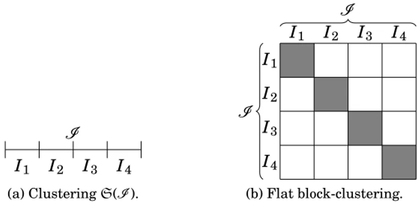
1.4.2.2 Flat and hierarchical block-clusterings . . . 38
1.4.2.3 Low-rank formats with nested basis . . . 42
1.4.2.4 Taxonomy of low-rank formats . . . 44
1.4.3 Using low-rank formats within sparse direct solvers . . . 45
1.4.3.1 Block-clustering of the fronts . . . 45
1.4.3.2 Full-rank or low-rank assembly? . . . 47
1.5 Experimental setting . . . 47
1.5.1 The MUMPS solver . . . 47
1.5.1.1 Main features . . . 48
1.5.1.2 Implementation details . . . 48
1.5.2 Test problems . . . 49
1.5.2.1 PDE generators . . . 49
1.5.2.2 Main set of real-life problems . . . 50
1.5.2.3 Complementary test problems . . . 51
1.5.3 Computational systems . . . 52
2 The Block Low-Rank Factorization 55 2.1 Offline compression: the FSUC variant . . . 56
2.2 The standard BLR factorization: the FSCU and UFSC variants . . . 56
2.2.1 The standard FSCU variant . . . 56
2.2.2 The Left-looking UFSC variant . . . 57
2.2.3 How to handle numerical pivoting in the BLR factorization . 58 2.2.4 Is the UFSC standard variant enough? . . . 61
2.3 Compress before Solve: the UFCS and UCFS variants . . . 62
2.3.1 When pivoting can be relaxed: the UFCS variant . . . 62
2.3.2.1 Algorithm description . . . 63
2.3.2.2 Dealing with postponed and delayed pivots . . . 65
2.3.2.3 Experimental study on matrices that require numer-ical pivoting . . . 67
2.4 Compress as soon as possible: the CUFS variant . . . 71
2.5 Compressing the contribution block . . . 73
2.6 Low-rank Updates Accumulation and Recompression (LUAR) . . . . 74
2.7 Chapter conclusion . . . 75
3 Strategies to add and recompress low-rank matrices 77 3.1 When: non-lazy, half-lazy, and full-lazy strategies . . . 78
3.2 What: merge trees . . . 79
3.2.1 Merge tree complexity analysis . . . 80
3.2.1.1 Uniform rank complexity analysis . . . 81
3.2.1.2 Non-uniform rank complexity analysis . . . 82
3.2.2 Improving the recompression by sorting the nodes . . . 84
3.3 How: merge strategies . . . 86
3.3.1 Weight vs geometry recompression . . . 86
3.3.2 Exploiting BOC leaf nodes . . . 87
3.3.3 Merge kernels . . . 88
3.3.4 Exploiting BOC general nodes . . . 89
3.4 Recompression strategies for the CUFS variant . . . 91
3.5 Experimental results on real-life sparse problems . . . 93
3.6 Chapter conclusion . . . 94
4 Complexity of the BLR Factorization 97 4.1 Context of the study . . . 98
4.2 From Hierarchical to BLR bounds . . . 99
4.2.1 H -admissibility and properties . . . 99
4.2.2 Why this result is not suitable to compute a complexity bound for BLR . . . 101
4.2.3 BLR-admissibility and properties . . . 101
4.3 Complexity of the dense standard BLR factorization . . . 106
4.4 From dense to sparse BLR complexity . . . 108
4.4.1 BLR clustering and BLR approximants of frontal matrices . . 109
4.4.2 Computation of the sparse BLR multifrontal complexity . . . 110
4.5 The other BLR variants and their complexity . . . 110
4.6 Numerical experiments . . . 114
4.6.1 Description of the experimental setting . . . 115
4.6.2 Flop complexity of each BLR variant . . . 115
4.6.3 LUAR and CUFS complexity . . . 116
4.6.4 Factor size complexity . . . 118
4.6.5 Low-rank threshold . . . 119
4.6.6 Block size . . . 122
4.7 Chapter conclusion . . . 122
5.1 Experimental setting . . . 125
5.1.1 Test machines . . . 125
5.1.2 Test problems . . . 126
5.2 Performance analysis of sequential FSCU algorithm . . . 126
5.3 Multithreading the BLR factorization . . . 128
5.3.1 Performance analysis of multithreaded FSCU algorithm . . . 128
5.3.2 Exploiting tree-based multithreading . . . 130
5.3.3 Right-looking vs. Left-looking . . . 132
5.4 BLR factorization variants . . . 133
5.4.1 LUAR: Low-rank Updates Accumulation and Recompression 134 5.4.2 UFCS algorithm . . . 136
5.5 Complete set of results . . . 137
5.5.1 Results on the complete set of matrices . . . 137
5.5.2 Results on 48 threads . . . 140
5.5.3 Impact of bandwidth and frequency on BLR performance . . . 141
5.6 Chapter conclusion . . . 143
6 Distributed-memory BLR Factorization 145 6.1 Parallel MPI framework and implementation . . . 145
6.1.1 General MPI framework . . . 145
6.1.2 Implementation in MUMPS . . . 147
6.1.3 Adapting this framework/implementation to BLR factorizations148 6.2 Strong scalability analysis . . . 150
6.3 Communication analysis . . . 152
6.3.1 Theoretical analysis of the volume of communications . . . 153
6.3.2 Compressing the CB to reduce the communications . . . 156
6.4 Load balance analysis . . . 158
6.5 Distributed-memory LUAR . . . 161
6.6 Distributed-memory UFCS . . . 162
6.7 Complete set of results . . . 163
6.8 Chapter conclusion . . . 163
7 Application to real-life industrial problems 165 7.1 3D frequency-domain Full Waveform Inversion . . . 165
7.1.1 Applicative context . . . 165
7.1.2 Finite-difference stencils for frequency-domain seismic mod-eling . . . 168
7.1.3 Description of the OBC dataset from the North Sea . . . 169
7.1.3.1 Geological target . . . 170
7.1.3.2 Initial models . . . 170
7.1.3.3 FWI experimental setup . . . 170
7.1.4 Results . . . 174
7.1.4.1 Nature of the modeling errors introduced by the BLR solver . . . 174
7.1.4.2 FWI results . . . 175
7.1.4.3 Computational cost . . . 176
7.2 3D Controlled-source Electromagnetic inversion . . . 185
7.2.1 Applicative context . . . 185
7.2.2 Finite-difference electromagnetic modeling . . . 186
7.2.3 Models and system matrices . . . 188
7.2.4 Choice of the low-rank thresholdε . . . . 190
7.2.5 Deep water versus shallow water: effect of the air . . . 194
7.2.6 Suitability of BLR solvers for inversion . . . 197
7.2.7 Section conclusion . . . 198
8 Comparison with an HSS solver: STRUMPACK 201 8.1 The STRUMPACK solver . . . 201
8.2 Complexity study . . . 202
8.2.1 Theoretical complexity . . . 202
8.2.2 Flop complexity . . . 202
8.2.3 Factor size complexity . . . 203
8.2.4 Influence of the low-rank threshold on the complexity . . . 204
8.3 Low-rank factor size and flops study . . . 205
8.4 Sequential performance comparison . . . 205
8.4.1 Comparison of the full-rank direct solvers . . . 205
8.4.2 Comparison of the low-rank solvers used as preconditioners . 205 8.5 Discussion . . . 209
9 Future challenges for large-scale BLR solvers 213 9.1 BLR analysis phase . . . 213
9.2 BLR solution phase . . . 216
9.3 Memory consumption of the BLR solver . . . 218
9.4 Results on very large problems . . . 220
Conclusion 223
Publications related to the thesis 229
List of most common
abbreviations and symbols
BLAS Basic Linear Algebra Subroutines
BLR Block Low-Rank
CB Contribution block FR/LR Full-rank/Low-rank
FSCU Factor–Solve–Compress–Update (and similarly for other variants)
H Hierarchical
HBS Hierarchically Block-Separable
HODLR Hierarchically Off-Diagonal Low-Rank HSS Hierarchically Semi-Separable
LUAR Low-rank updates accumulation and recompression
MF Multifrontal
RL/LL Right-looking/Left-looking
UFSMC University of Florida Sparse Matrix Collection Ai, j (i, j)−th entry of matrix A
Ai,: i−th row of matrix A A:, j j−th column of matrix A [a, b] continuous interval from a to b [a; b] discrete interval from a to b
List of Algorithms
1.1 Dense LU (Right-looking) factorization (without pivoting) . . . 8
1.2 Dense block LU (Right-looking) factorization (without pivoting) . . . 8
1.3 Dense tile LU (Right-looking) factorization (without pivoting) . . . 9
1.4 Dense tile LU (Left-looking) factorization (without pivoting) . . . 10
1.5 Dense tile LDLT (Right-looking) factorization (without pivoting) . . . 10
1.6 Dense tile LU solution (without pivoting) . . . 12
1.7 Dense tile LU factorization (with pivoting) . . . 15
1.8 Factor+Solve step (unsymmetric case) . . . 16
1.9 Factor+Solve step adapted to frontal matrices (unsymmetric case) . . 29
1.10 Iterative refinement . . . 31
1.11 Multifrontal solution phase (without pivoting). . . 32
2.1 Frontal BLR LDLT (Right-looking) factorization: FSCU variant. . . . 57
2.2 Right-lookingRL-Updatestep. . . 57
2.3 Frontal BLR LDLT (Left-looking) factorization: UFSC variant. . . 58
2.4 Left-lookingLL-Updatestep. . . 58
2.5 Frontal BLR LDLT (Left-looking) factorization: UFCS variant. . . 63
2.6 Frontal BLR LDLT (Left-looking) factorization: UCFS variant. . . 64
2.7 Factor+Solve step adapted for the UCFS factorization (symmetric case) 66 2.8 Frontal BLR LDLT (left-looking) factorization: CUFS variant. . . 71
2.9 CUFS-Updatestep. . . 72
2.10 LUAR-Updatestep. . . 74
3.1a Full-lazy recompression. . . 79
List of Tables
1.1 Theoretical complexity of the multifrontal factorization. . . 27
1.2 Taxonomy of existing low-rank formats. . . 44
1.3 Main set of matrices and their Full-Rank statistics. . . 51
1.4 Complementary set of matrices and their Full-Rank statistics. . . 52
2.1 The Block Low-Rank factorization variants. . . 55
2.2 Set of matrices that require pivoting. . . 69
2.3 Comparison of the UFSC, UFCS, and UCFS factorization variants. . . . 70
3.1 Full-, half-, and non-lazy recompression. . . 78
3.2 Impact of sorting the nodes for different merge trees. . . 84
3.3 Exploiting weight and geometry information. . . 87
3.4 Usefulness of exploiting the orthonormality for different merge trees. . . 88
3.5 Input and output of different merge kernels. . . 90
3.6 Usefulness of exploiting the orthonormality for different merge kernels. 91 4.1 Main operations for the UFSC factorization. . . 107
4.2 Flop and factor size complexity of the UFSC variant. . . 111
4.3 Main operations for the other factorization variants. . . 112
4.4 Flop and factor size complexity of the other variants. . . 113
4.5 Complexity of BLR multifrontal factorization. . . 114
4.6 Complexity of BLR multifrontal factorization (r = O (1) and O (pm)). . . . 114
4.7 Number of full-, low-, and zero-rank blocks. . . 121
5.1 List of machines and their properties. . . 126
5.2 Sequential run (1 thread) on matrix S3. . . 127
5.3 Performance analysis of sequential run on matrix S3. . . 127
5.4 Multithreaded run on matrix S3. . . 129
5.5 Performance analysis of multithreaded run on matrix S3. . . 129
5.6 FR and BLR times exploiting both node and tree parallelism. . . 131
5.7 FR and BLR times in Right- and Left-looking. . . 132
5.8 Performance analysis of the UFSC+LUAR factorization. . . 134
5.9 Performance and accuracy of UFSC and UFCS variants. . . 136
5.11 Multicore results on complete set of matrices (1/2). . . 138
5.12 Multicore results on complete set of matrices (2/2). . . 139
5.13 Results on 48 threads. . . 141
5.14 brunch and grunch BLR time comparison. . . . 142
6.1 Strong scalability analysis on matrix 10Hz. . . 151
6.2 Volume of communications for the FR and BLR factorizations. . . 152
6.3 Theoretical communication analysis: dense costs. . . 154
6.4 Theoretical communication analysis: sparse costs. . . 156
6.5 Performance of the CBFRand CBLRBLR factorizations. . . 157 6.6 Volume of communications for the CBFRand CBLRBLR factorizations. . 157 6.7 Improving the mapping with BLR asymptotic complexity estimates. . . . 159
6.8 Influence of the splitting strategy on the FR and BLR factorizations. . . 160
6.9 Performance of distributed-memory LUAR factorization. . . 161
6.10 Performance and accuracy of UFSC and UFCS variants. . . 162
6.11 Distributed-memory results on complete set of matrices. . . 163
7.1 North Sea case study: problem size and computational resources. . . 174
7.2 North Sea case study: BLR modeling error. . . 174
7.3 North Sea case study: BLR computational savings. . . 177
7.4 North Sea case study: FWI cost. . . 178
7.5 North Sea case study: projected BLR computational savings. . . 179
7.6 Problem sizes. . . 190
7.7 Shallow- vs deep-water results. . . 194
7.8 Suitability of BLR solvers for inversion. . . 198
8.1 Theoretical complexity of the BLR and HSS multifrontal factorization. . 202
8.2 Best tolerance choice for BLR and HSS solvers. . . 209
9.1 Influence of the halo depth parameter. . . 214
9.2 Acceleration of the BLR clustering with multithreading. . . 215
9.3 Memory consumption analysis of the FR and BLR factorizations. . . 218
9.4 Set of very large problems: full-rank statistics. . . 220
9.5 Set of very large problems: low-rank statistics. . . 220
9.6 Very large problems: total memory consumption . . . 221
List of Figures
1.1 Example of a 5-point stencil finite-difference mesh. . . 6
1.2 Part of the matrix that is updated in the symmetric case. . . 11
1.3 Dense triangular solution algorithms. . . 12
1.4 LINPACK and LAPACK pivoting styles (unsymmetric case). . . 17
1.5 LINPACK and LAPACK pivoting styles (symmetric case). . . 17
1.6 Symbolic factorization. . . 19
1.7 Nested dissection. . . 20
1.8 Symbolic factorization with nested dissection reordering. . . 21
1.9 Construction of the elimination tree. . . 22
1.10 Right-looking, left-looking, and multifrontal approaches. . . 24
1.11 Three examples of frontal matrices. . . 25
1.12 Assembly tree. . . 26
1.13 Frontal solution phase. . . 31
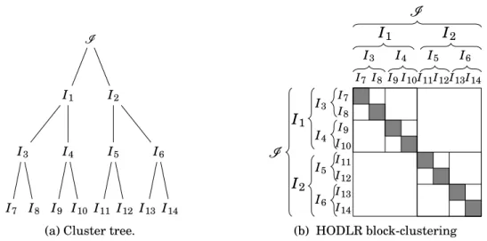
1.14 Block-admissibility condition. . . 37 1.15 Flat block-clustering. . . 39 1.16 HODLR block-clustering. . . 41 1.17 H block-clustering. . . 42 1.18 HSS tree. . . 44 1.19 Halo-based partitioning. . . 46
1.20 Low-rank extend-add operation. . . 47
2.1 BLR factorization with numerical pivoting scheme. . . 59
2.2 LINPACK and LAPACK pivoting styles in BLR (symmetric case). . . 60
2.3 LAPACK pivoting style in BLR, with postponed pivots (symmetric case). 60
2.4 LR-swap strategy. . . 61
2.5 Column swap in the UCFS factorization. . . 65
2.6 Strategies to merge postponed pivots (UCFS factorization). . . 67
2.7 Low-rank Updates Accumulation and Recompression. . . 75
3.1 Merge trees comparison. . . 80
3.2 Comparison of star and comb tree recompression for non-uniform rank distributions. . . 83
3.4 Impact of sorting the leaves of the merge tree. . . 85
3.5 Merge kernels comparison. . . 92
3.6 Gains due to LUAR on real-life sparse problems. . . 94
4.1 Illustration of the BLR-admissibility condition. . . 102
4.2 Illustration of Lemma4.1(proof of the boundedness of Nna). . . 103 4.3 BLR clustering of the root separator of a 1283Poisson problem. . . 109
4.4 Flop complexity of each BLR variant (Poisson,ε = 10−10). . . 116
4.5 Flop complexity of each BLR variant (Helmholtz,ε = 10−4). . . 117
4.6 Flop complexity of the UFCS+LUAR variant (Poisson,ε = 10−10). . . . . 118 4.7 Flop complexity of the CUFS variant (Poisson,ε = 10−10). . . 118
4.8 Factor size complexity with METIS ordering. . . 119
4.9 Flop complexities for different thresholdsε (Poisson problem). . . . 120
4.10 Flop complexities for different thresholdsε (Helmholtz problem). . . . . 120
4.11 Factor size complexities for different thresholdsε. . . . 121
4.12 Influence of the block size on the complexity. . . 123
5.1 Normalized flops and time on matrix S3. . . 128
5.2 Illustration of how both node and tree multithreading can be exploited. . 130
5.3 Memory access pattern in the RL and LL BLR Update. . . 133
5.4 Performance benchmark of the Outer Product step on brunch. . . . 135
5.5 Summary of multicore performance results. . . 140
5.6 Roofline model analysis of the Outer Product operation. . . 142
6.1 MPI framework based on both tree and node parallelism. . . 146
6.2 MPI node parallelism framework. . . 146
6.3 Illustration of tree and node parallelism. . . 147
6.4 Splitting of a front into a split chain. . . 148
6.5 LU and CB messages. . . 148
6.6 BLR clustering constrained by MPI partitioning. . . 149
6.7 CB block mapped on two processes on the parent front. . . 150
6.8 Strong scalability of the FR and BLR factorizations (10Hz matrix). . . . 151
6.9 Volume of communications as a function of the front size. . . 154
7.1 North Sea case study: acquisition layout. . . 171
7.2 North Sea case study: FWI model depth slices. . . 172
7.3 North Sea case study: FWI model vertical slices. . . 173
7.4 North Sea case study: BLR modeling errors (5Hz frequency). . . 180
7.5 North Sea case study: BLR modeling errors (7Hz frequency). . . 181
7.6 North Sea case study: BLR modeling errors (10Hz frequency). . . 182
7.7 North Sea case study: data fit achieved with the BLR solver. . . 183
7.8 North Sea case study: misfit function versus iteration number. . . 184
7.9 H-model. . . 188
7.10 SEAM model. . . 189
7.11 Relative residual normδ. . . . 192
7.12 Relative difference between the FR and BLR solutions. . . 193
7.13 Flop complexity for shallow- and deep-water matrices. . . 195
8.1 BLR and HSS flop complexity comparison. . . 203
8.2 BLR and HSS factor size complexity comparison. . . 204
8.3 Size of BLR and HSS low-rank factors. . . 206
8.4 Flops for BLR and HSS factorizations. . . 207
8.5 How the weak-admissibility condition can result in higher storage. . . . 208
8.6 MUMPS and STRUMPACK sequential full-rank comparison. . . 208
8.7 MUMPS and STRUMPACK sequential low-rank comparison. . . 210
8.8 Which solver is the most suited in which situation? . . . 211
9.1 BLR right- and left-looking frontal forward elimination. . . 217
Introduction
We are interested in efficiently computing the solution of a large sparse system of linear equations:
Ax = b,
where A is a square sparse matrix of order n, and x and b are the unknown and right-hand side vectors. This work focuses on the solution of this problem by means of direct, factorization-based methods, and in particular based on the multifrontal approach (Duff and Reid, 1983).
Direct methods are widely appreciated for their numerical robustness, reliabil-ity, and ease of use. However, they are also characterized by their high tional complexity: for a three-dimensional problem, the total amount of computa-tions and the memory consumption are proportional to O(n2) and O(n4/3), respec-tively (George, 1973). This limits the scope of direct methods on very large problems (matrices with hundreds of millions of unknowns).
The goal of this work is to reduce the cost of sparse direct solvers without sacri-ficing their robustness, ease of use, and performance.
In numerous scientific applications, such as the solution of partial differential equations, the matrices resulting from the discretization of the physical problem have been shown to possess a low-rank property (Bebendorf, 2008): well-defined off-diagonal blocks B of their Schur complements can be approximated by low-rank products B = X Ye T ≈ B. This property can be exploited in multifrontal solvers to provide a substantial reduction of their complexity.
Several matrix representations, so-called low-rank formats, have been proposed to exploit this property within multifrontal solvers. The H -matrix format ( Hack-busch, 1999), where H stands for hierarchical, has been widely studied in the literature, as well as its variants H2 (Börm, Grasedyck, and Hackbusch, 2003), HSS (Xia, Chandrasekaran, Gu, and Li, 2010), and HODLR (Aminfar, Ambikasaran, and Darve, 2016).
In the hierarchical framework, the matrix is hierarchically partitioned in order to maximize the low-rank compression rate; this can lead to a theoretical com-plexity of the multifrontal factorization as low as O(n), both in flops and memory consumption. However, because of the hierarchical structure of the matrix, it is not straightforward to use in a general purpose, algebraic “black-box” solver, and to achieve high performance.
Alternatively, a so-called Block Low-Rank (BLR) format has been put forward by Amestoy et al. (2015a). In the BLR framework, the matrix is partitioned by means of a flat, non-hierarchical blocking of the matrix. The simpler structure of the BLR format makes it easy to use in a parallel, algebraic solver. Amestoy et al. (2015a)also introduced the “standard” BLR factorization variant, which can easily handle numerical pivoting, a critical feature often lacking in other low-rank solvers. Despite these advantages, the BLR format was long dismissed due to its un-known theoretical complexity; it was even conjectured it could asymptotically be-have as the full-rankO(n2) solver. One of the main contributions of this thesis is to investigate the complexity of the BLR format and to prove it is in fact asymp-totically lower thanO(n2). We show that the theory for hierarchical matrices does not provide a satisfying result when applied to BLR matrices (thereby justifying the initial pessimistic conjecture). We extend the theory to compute the theoretical complexity of the BLR multifrontal factorization. We show that the standard BLR variant ofAmestoy et al. (2015a)can lead to a complexity as low asO(n5/3) in flops andO(nlog n) in memory. Furthermore, we introduce new BLR variants that can further reduce the flop complexity, down to O(n4/3). We provide an experimental study with numerical results to support our complexity bounds.
The modifications introduced by the BLR variants can be summarized as fol-lows:
• During the factorization, the sum of many low-rank matrices arises in the up-date of the trailing submatrix. We propose an algorithm, referred to as low-rank updates accumulation and recompression (LUAR), to accumulate and recompress these low-rank updates together, which improves both the perfor-mance and complexity of the factorization. We provide an in-depth analysis of the different recompression strategies that can be considered.
• The compression can be performed at different stages of the BLR factoriza-tion. In the standard variant, it is performed relatively late so that only part of the operations are accelerated. We propose novel variants that perform the compression earlier in order to further reduce the complexity of the factoriza-tion. In turn, we also show that special care has to be taken to maintain the ability to perform numerical pivoting.
Our complexity analysis, together with the improvements brought by the BLR variants, therefore shows that BLR multifrontal solvers can achieve a low theoret-ical complexity.
However, achieving low complexity is only half the work necessary to tackle creasingly large problems. In a context of rapidly evolving architectures, with an in-creasing number of computational resources, translating the complexity reduction into actual performance gains on modern architectures is a challenging problem. We first present a multithreaded BLR factorization, and analyze its performance in shared-memory multicore environments on a large set of problems coming from a variety of real-life applications. We put forward several algorithmic properties of the BLR variants necessary to efficiently exploit multicore systems by improving the efficiency and scalability of the BLR factorization. We then present and
ana-lyze the distributed-memory BLR factorization, for which additional challenges are identified; some solutions are proposed.
The algorithms presented throughout this thesis have been implemented within the MUMPS (Amestoy, Duff, Koster, and L’Excellent, 2001;Amestoy, Guermouche, L’Excellent, and Pralet, 2006;Amestoy et al., 2011) solver. We illustrate the use of our approach in three industrial applications coming from geosciences and struc-tural mechanics. We also compare our solver with the STRUMPACK (Rouet, Li, Ghysels, and Napov, 2016; Ghysels, Li, Rouet, Williams, and Napov, 2016; Ghy-sels, Li, Gorman, and Rouet, 2017) solver, based on Hierarchically Semi-Separable approximations, to shed light on the differences between these formats. We com-pare their usage as accurate, high precision direct solvers and as more approxi-mated, fast preconditioners coupled with an iterative solver. Finally, we conclude this thesis by discussing some future challenges that await BLR solvers for large-scale systems and applications. We propose some ways to tackle these challenges, and illustrate them by reporting results on very large problems (up to 130 million unknowns).
The remainder of this thesis is organized as follows. In order to make the thesis self-contained, we provide in Chapter1general background on numerical linear al-gebra, and more particularly sparse direct methods and low-rank approximations. Chapter 2 is central to this work. It articulates and describes in detail the Block Low-Rank (multifrontal) factorization in all its variants. Chapter3provides an in-depth analysis of the different strategies to perform the so-called LUAR algorithm. Chapter 4 deals with the theoretical aspects regarding the complexity of the BLR factorization, including the proof that it is asymptotically lower than that of the full-rank solver, together with its computation for all BLR variants and experimen-tal validation. Chapters5and6focus on the performance of the BLR factorization on shared-memory (multicore) and distributed-memory architectures, respectively. The BLR variants are shown to improve the performance and scalability of the fac-torization. Then, two real-life applications which benefit from BLR approximations are studied in Chapter7. Chapter8provides an experimental comparison with the HSS solver STRUMPACK. Chapter 9tackles the solution of a very large problem, to show the remaining challenges of BLR solvers at scale. Finally, we conclude the manuscript by summarizing the main results, and mentioning some perspectives.
C
HAPTER1
General Background
We are interested in efficiently computing the solution of a large sparse system of linear equations
Ax = b, (1.1)
where A is a square sparse matrix of order n, x is the unknown vector of size n, and b is the right-hand side vector of size n.
In this chapter, we give an overview of existing methods to solve this prob-lem and provide some background that will be useful throughout the thesis. To achieve this objective, we consider an illustrative example (2D Poisson’s equation) and guide the reader through the steps of its numerical solution.
1.1
An illustrative example: PDE solution
We consider the solution of Poisson’s equation inRd
∆u = f , (1.2)
where ∆is the Laplace operator, also noted ∇2, defined in two-dimensional Carte-sian coordinates as ∆u(x, y) = µ ∂2 ∂2x+ ∂2 ∂2y ¶ u(x, y). (1.3)
Equation (1.2) is therefore a partial derivative equation (PDE).
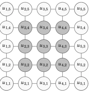
While this particular equation has an analytical solution on simple domains, our purpose here is to use it as an illustrative example to describe the solution of general PDEs on more complicated domains. We are thus interested in computing an approximate solution restricted to a subset of discrete points. Two widely used approaches to compute such a solution are the finite-difference method and the finite-element method, which consist in discretizing the system using a subset of points (or polygons) forming a mesh. In the following, we consider as an example a finite-difference discretization resulting in a 5 × 5 regular equispaced mesh, as illustrated in Figure1.1.
The function u is then approximated by a vector, also noted u, whose elements ui, j correspond to the value of u at the mesh points (i, j). f is similarly
approxi-u2,2 u2,3 u2,4 u3,2 u3,3 u3,4 u4,2 u4,3 u4,4 u1,1 u1,2 u1,3 u1,4 u1,5 u5,1 u5,2 u5,3 u5,4 u5,5 u1,1 u2,1 u3,1 u4,1 u5,1 u1,5 u2,5 u3,5 u4,5 u5,5
Figure 1.1 – Example of a 5-point stencil finite-difference mesh. The boundary nodes (light color) are used to compute the approximate derivatives at the interior nodes (dark color) but are not part of the linear system solved.
mated. The next step is to approximate the partial derivatives of u at a given point (x, y) of the mesh, which can be done (using the central step method) as follows:
∂ ∂xu(x, y) ≈ u(x + h, y) − u(x − h, y) 2h , (1.4) ∂ ∂yu(x, y) ≈ u(x, y + h) − u(x, y − h) 2h , (1.5)
where the grid size is h in both dimensions, and should be taken small enough for the approximation to be accurate. Furthermore, second order derivatives can also be approximated:
∂2
∂2xu(x, y) ≈
u(x + h, y) − 2u(x, y) + u(x − h, y)
h2 , (1.6)
∂2
∂2yu(x, y) ≈
u(x, y + h) − 2u(x, y) + u(x, y − h)
h2 . (1.7)
Therefore, the Laplacian operator in two dimensions can be approximated as
∆u(x, y) ≈ 1
h2(u(x + h, y) + u(x − h, y) + u(x, y + h) + u(x, y − h) − 4u(x, y)), (1.8) which is known as the five-point stencil finite-difference method.
Equation (1.2) can thus be approximated by the discrete Poisson equation (∆u)i, j=
1
h2(ui+1, j+ ui−1, j+ ui, j+1+ ui, j−1− 4ui, j) = fi, j, (1.9) where i, j ∈ [2; N−1]; N is the number of grid points. Note that the approximation of the Laplacian at node (i, j) requires the values of u at the neighbors in all directions;
therefore, in practice, the boundary nodes are prescribed and the equation is solved for the interior points only. In this case, equation (1.9) is equivalent to a linear system Au = g where u contains the interior nodes (shaded nodes in Figure 1.1), and A is a block-diagonal matrix of order (N − 2)2 of the form
A = D −I 0 · · · 0 −I D . .. ... ... 0 . .. ... ... 0 .. . . .. ... D −I 0 · · · 0 −I D , (1.10)
where I is the identity matrix of order N − 2 and D, also of order N − 2, is a tridiag-onal matrix of the form
D = 4 −1 0 · · · 0 −1 4 . .. ... ... 0 . .. ... ... 0 .. . . .. ... 4 −1 0 · · · 0 −1 4 . (1.11)
Finally, we have g = −h2f + β, where β contains the boundary nodes information. For example, with the mesh of Figure1.1, we obtain the following 9 × 9 linear system: 4 −1 0 −1 0 0 0 0 0 −1 4 −1 0 −1 0 0 0 0 0 −1 4 −1 0 −1 0 0 0 −1 0 −1 4 −1 0 −1 0 0 0 −1 0 −1 4 −1 0 −1 0 0 0 −1 0 −1 4 −1 0 −1 0 0 0 −1 0 −1 4 −1 0 0 0 0 0 −1 0 −1 4 −1 0 0 0 0 0 −1 0 −1 4 u2,2 u3,2 u4,2 u2,3 u3,3 u4,3 u2,4 u3,4 u4,4 = −h2f2,2+ u1,2+ u2,1 −h2f3,2+ u3,1 −h2f4,2+ u5,2+ u4,1 −h2f2,3+ u1,3 −h2f3,3 −h2f4,3+ u5,3 −h2f2,4+ u1,4+ u2,5 −h2f3,4+ u3,5 −h2f4,4+ u5,4+ u4,5 . (1.12)
We now discuss how to solve such a linear system. There are two main classes of methods:
• Iterative methods build a sequence of iterates xk which hopefully converges towards the solution. Although they are relatively cheap in terms of memory and computations, their effectiveness strongly depends on the ability to find a good preconditioner to ensure convergence.
• Direct methods build a factorization of matrix A (e.g. A = LU or A = QR) to solve directly the system. While they are commonly appreciated for their numerical robustness, reliability, and ease of use, they are however also char-acterized by a large amount of memory consumption and computations. In this thesis, we focus on direct methods based on Gaussian elimination, i.e. methods that factorize A as LU (general case), LDLT (symmetric indefinite case),
or LLT (symmetric positive case, also known as Cholesky factorization). We first give an overview of these methods in the dense case.
1.2
Dense LU or LDL
Tfactorization
1.2.1
Factorization phase
1.2.1.1 Point, block, and tile algorithms
The LU factorization of a dense matrix A, described in Algorithm1.1, computes the decomposition A = LU, where L is unit lower triangular and U is upper trian-gular. At each step k of the factorization, a new column of L and a new row of U are computed; we call the diagonal entry Ak,k a pivot and step k its elimination.
Algorithm 1.1 Dense LU (Right-looking) factorization (without pivoting)
1: /*Input: a matrix A of order n */
2: for k = 1 to n − 1 do 3: Ak+1:n,k← Ak+1:n,k/Ak,k
4: Ak+1:n,k+1:n← Ak+1:n,k+1:n− Ak+1:n,kAk,k+1:n
5: end for
Algorithm 1.1 is referred to as in-place because A is overwritten during the factorization: its lower triangular part is replaced by L and its upper triangular part by U (note that its diagonal contains the diagonal of U, as the diagonal of L is not explicitly stored since Li,i= 1).
Algorithm1.1is also referred to as point because the operations are performed on single entries of the matrix. This means the factorization is mainly performed with BLAS-2 operations. Its performance can be substantially improved (typically by an order of magnitude) by using BLAS-3 operations instead, which increase data locality (i.e. cache reuse) (Dongarra, Du Croz, Hammarling, and Duff, 1990). For this purpose, the operations in Algorithm1.1 can be reorganized to be performed on blocks of entries: the resulting algorithm is referred to as block LU factorization and is described in Algorithm1.2.
Algorithm 1.2 Dense block LU (Right-looking) factorization (without pivoting)
1: /*Input: a p × p block matrix A of order n; A = [Ai, j]i, j∈[1;p] */
2: for k = 1 to p do 3: Factor: Ak,k← Lk,kUk,k 4: Solve (L): Ak+1:p,k← Ak+1:p,kUk,k−1 5: Solve (U): Ak,k+1:p← L−1 k,kAk,k+1:p 6: Update: Ak:p,k:p← Ak:p,k:p− Ak:p,kAk,k:p 7: end for
The block LU factorization consists of three main steps: Factor, Solve, and Up-date. The Factor step is performed by means of a point LU factorization (Algo-rithm 1.1). The Solve step takes the form of a triangular solve (so-called trsm
(so-calledgemmkernel). Therefore, both the Solve and Update rely on BLAS-3 oper-ations.
The LU factorization can be accelerated when several cores are available by using multiple threads. Both the point and block LU factorizations, as implemented for example in LAPACK (Anderson et al., 1995), solely rely on multithreaded BLAS kernels to multithread the factorization.
More advanced versions (Buttari, Langou, Kurzak, and Dongarra, 2009; Quintana-Ortí, Quintana-Quintana-Ortí, Geijn, Zee, and Chan, 2009) of Algorithm 1.2 have been de-signed by decomposing the matrix into tiles, where each tile is stored contiguously in memory. This algorithm, described in Algorithm1.3, is referred to as tile LU fac-torization, and is usually associated with a task-based multithreading which fully takes advantage of the independencies between computations. In this work, we will not consider task-based factorizations but will discuss tile factorizations be-cause they are the starting point to the BLR factorization algorithm, as explained in Chapter2.
Algorithm 1.3 Dense tile LU (Right-looking) factorization (without pivoting)
1: /*Input: a p × p tile matrix A of order n; A = [Ai, j]i, j∈[1;p] */
2: for k = 1 to p do
3: Factor: Ak,k← Lk,kUk,k
4: for i = k + 1 to p do
5: Solve (L): Ai,k← Ai,kUk,k−1
6: Solve (U): Ak,i← L−1 k,kAk,i 7: end for 8: for i = k + 1 to p do 9: for j = k + 1 to p do 10: Update: Ai, j← Ai, j− Ai,kAk, j 11: end for 12: end for 13: end for
For the sake of conciseness, in the following, we will present the algorithms in their tile version. Unless otherwise specified, the discussion also applies to block algorithms.
The number of operations and memory required to perform the LU factorization is independent of the strategy used (point, block, or tile) and are equal toO(n3) and O(n2), respectively (Golub and Van Loan, 2012).
1.2.1.2 Right-looking vs Left-looking factorization
Algorithms1.1,1.2, and1.3are referred to as right-looking, in the sense that as soon as column k is eliminated, the entire trailing submatrix (columns to its “right”) is updated. These algorithms can be rewritten in a left-looking form, where at each step k, column k is updated using all the columns already computed (those at its “left”) and then eliminated.
The tile version of the Left-looking LU factorization is provided in Algorithm1.4
Algorithm 1.4 Dense tile LU (Left-looking) factorization (without pivoting)
1: /*Input: a p × p block matrix A of order n; A = [Ai, j]i, j∈[1;p] */
2: for k = 1 to p do 3: for i = k to p do 4: for j = 1 to k − 1 do
5: Update (L): Ai,k← Ai,k− Ai, jAj,k
6: if i 6= k then
7: Update (U): Ak,i← Ak,i− Ak, jAj,i
8: end if
9: end for
10: end for
11: Factor: Ak,k← Lk,kUk,k
12: for i = k + 1 to p do
13: Solve (L): Ai,k← Ai,kUk,k−1
14: Solve (U): Ak,i← L−1 k,kAk,i
15: end for
16: end for
1.2.1.3 Symmetric case
In the symmetric case, the matrix is decomposed in LDLT, where L is a unit lower triangular matrix and D a diagonal (or block-diagonal, in the case of pivoting, as explained in Section1.2.4.1) matrix.
When the matrix is positive definite, it can even be decomposed in LLT(where L is not unit anymore), commonly referred to as Cholesky factorization. In this thesis, we will consider the more general symmetric indefinite case (LDLTdecomposition), but the discussion also applies to the Cholesky decomposition.
Algorithm 1.5 Dense tile LDLT(Right-looking) factorization (without pivoting)
1: /*Input: a p × p tile matrix A of order n; A = [Ai, j]i, j∈[1;p] */
2: for k = 1 to p do
3: Factor: Ak,k← Lk,kDk,kLTk,k
4: for i = k + 1 to p do 5: Solve: Ai,k← Ai,kL−T
k,kD−1k,k 6: end for 7: for i = k + 1 to p do 8: for j = k + 1 to i do 9: Update: Ai, j← Ai, j− Ai,kATj,k 10: end for 11: end for 12: end for
In Algorithm 1.5, we present the tile LDLT right-looking factorization. The other versions (block, left-looking) are omitted for the sake of conciseness. The algorithm is similar to the unsymmetric case, with the following differences:
• The Solve step still takes the form of a triangular solve, but also involves a column scaling with the inverse of D.
• Finally, since the matrix is symmetric, the Update is only done on its lower triangular part. In particular, note that in Algorithm 1.5, for the sake of simplicity, the diagonal blocks Ai,iare entirely updated (line9) when they are in fact lower triangular, which would thus result in additional flops. One could instead update each column one by one, minimizing the flops, but this would be very inefficient as it consists of BLAS-1 operations. In practice, one can find a compromise between flops and efficiency by further refining the diagonal blocks, which leads to a “staircase” update, as illustrated in Figure1.2.
Figure 1.2 – Part of the matrix that is updated in the symmetric case.
1.2.2
Solution phase
Once matrix A has been decomposed under the form LU, computing the solution x of equation (1.1) is equivalent to solve two linear systems:
Ax = LU x = b ⇔ ½
L y = b
U x = y , (1.13)
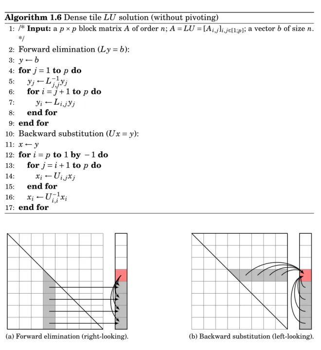
which can be achieved easily thanks to the special triangular form of L and U. The two solves L y = b and U x = y are respectively referred to as forward elim-ination and backward substitution. They are described, in their tile version, in Algorithm1.6.
Note that the right- and left-looking distinction also applies for the solution phase. In Algorithm 1.6, the forward elimination is written in its right-looking version while the backward substitution is written in left-looking.
1.2.3
Numerical stability
Once the solution x is computed, we may want to evaluate its quality. Indeed, computations performed on computers are inexact: they are subject to roundoff errors due to the floating-point representation of numbers. Thus, the linear system that is solved is in fact
Algorithm 1.6 Dense tile LU solution (without pivoting)
1: /*Input: a p × p block matrix A of order n; A = LU = [Ai, j]i, j∈[1;p]; a vector b of size n.
*/ 2: Forward elimination (L y = b): 3: y ← b 4: for j = 1 to p do 5: yj← L−1 j, jyj 6: for i = j + 1 to p do 7: yi← Li, jyj 8: end for 9: end for
10: Backward substitution (U x = y): 11: x ← y 12: for i = p to 1 by − 1 do 13: for j = i + 1 to p do 14: xi← Ui, jxj 15: end for 16: xi← Ui,i−1xi 17: end for
(a) Forward elimination (right-looking). (b) Backward substitution (left-looking).
Figure 1.3 – Dense triangular solution algorithms.
where δA, δx, and δb are called perturbations. An important aspect of any algo-rithm is to evaluate its stability. An algoalgo-rithm is said to be stable if small pertur-bations lead to a small error. Of course, this depends on how the error is measured. A first metric is to measure the quality of the computed solution ˜x with respect to the exact solution x, referred to as the forward error metric:
kx − ˜xk
kxk . (1.15)
The forward error can be large for two reasons: an unstable algorithm; or an ill-conditioned matrix (i.e., a matrix whose condition number is large), in which case even a stable algorithm can lead to a poor forward error.
To distinguish these two cases,Wilkinson (1963)introduces the backward error metric, which measures the smallest perturbationδA such that ˜x is the exact solu-tion of the perturbed system (A + δA) ˜x = b. The normwise backward error can be evaluated as (Rigal and Gaches, 1967):
kA ˜x − bk
kAkk ˜xk + kbk, (1.16)
which does not depend on the conditioning of the system. Its componentwise ver-sion (Oettli and Prager, 1964) will also be of interest in the sparse case:
max i
|A ˜x − b|i (|A|| ˜x| + |b|)i
. (1.17)
In this manuscript, we will use the (normwise and componentwise) backward error to measure the accuracy of our algorithms and we will refer to it as (normwise and componentwise) scaled residual.
It turns out Algorithm 1.1 is not backward stable. In particular, at step k, if Ak,k= 0, the algorithm will fail since line3would take the form of a division by zero. Furthermore, even if Ak,k is not zero but is very small in amplitude, Algorithm1.1 will lead to significant roundoff errors by creating too large off-diagonal entries in column and row k. This is measured by the growth factor.
One can partially overcome this issue by preprocessing the original matrix, e.g. by scaling the matrix so that its entries are of moderate amplitude (seeSkeel (1979)
and, for the sparse case,Duff and Pralet (2005)andKnight, Ruiz, and Uçar (2014)). However, in many cases, preprocessing strategies are not sufficient to ensure the numerical stability of the algorithm. In these cases, we need to perform numerical pivoting.
1.2.4
Numerical pivoting
The objective of numerical pivoting is to limit the growth factor by avoiding small pivots. The most conservative option is thus to select, at each step k, the entry Ai, jin the trailing submatrix of maximal amplitude:
Ai, j= max
i0, j0∈[k;n]|Ai0, j0|, (1.18)
and to permute row k with row i and column k with column j. This is referred to as complete pivoting (Wilkinson, 1961). It is however rarely used since it implies a significant amount of searching and swapping which can degrade the performance of the factorization. A more popular strategy, known as row or column partial pivot-ing, consists in restricting the search of the pivot on row k or column k, respectively:
Ak, j= max
j0∈[k;n]|Ak, j0| or Ai,k= maxi0∈[k;n]|Ai0,k|, (1.19)
and permute column k with column j, or row k with row i, respectively. In the literature, as well as in reference implementations such as LAPACK (Anderson et
al., 1995), column partial pivoting is often considered, and we will thus also consider it in the rest of this section, for the sake of clarity.
Partial pivoting can still lead to significant amounts of swapping and is there-fore sometimes relaxed by choosing a threshold τ and accepting some pivot Aj,k if
|Aj,k| ≥ τ max
i0∈[k;n]|Ai0,k|. (1.20)
This strategy, referred to as threshold partial pivoting (Duff, Erisman, and Reid, 1986), is often enough to ensure the stability of the factorization, typically with a threshold of the orderτ = 0.1 or τ = 0.01. It is of particular interest in the sparse case as explained in Section1.3.
1.2.4.1 Symmetric case
In the symmetric case, special care must be taken to avoid losing the symmetry of A by considering symmetric permutations only. However, in general, it is not always possible to find a safe pivot with symmetric permutations only. For example, consider the following symmetric matrix:
A = 0 2 1 2 0 2 1 2 0 .
At step 1, A1,1= 0 is not an acceptable pivot. Thus row 1 must be exchanged with row 2 or 3. In both cases, the symmetry of A is lost. For example, if rows 1 and 2 are exchanged, the resulting matrix is
2 0 2 0 2 1 1 2 0 ,
which is not symmetric anymore, since A1,36= A3,1(and A2,36= A3,2).
To ensure the stability of the factorization while maintaining the symmetry, two-by-two pivots (noted 2 × 2 pivots hereinafter) must be used (Bunch and Parlett, 1971). For example, the previous matrix can be factored as
A = LDLT= 1 0 0 0 1 0 1 12 1 0 2 0 2 0 0 0 0 −2 1 0 1 0 1 12 0 0 1 ,
where D is made of one 2 × 2 pivot, µ
0 2 2 0
, and one 1 × 1 pivot, −2. Thus D is not diagonal anymore but block-diagonal.
Many strategies have been proposed in the literature to search and choose 2 × 2 pivots. The Bunch-Parlett algorithm (Bunch and Parlett, 1971) uses a complete piv-oting strategy to scan the entire trailing submatrix at each step to search the best possible 2 × 2 pivot; it is a backward stable algorithm and also leads to bounded en-tries in L, but it is also expensive and requires a point factorization to be used. On
the contrary, the Bunch-Kaufman (Bunch and Kaufman, 1977) algorithm is based on partial pivoting, scanning at most two columns/rows at each step, which makes it cheaper and allows the use of block or tile factorizations; it is a backward sta-ble algorithm but may lead to unbounded entries in L. For this reason, Ashcraft, Grimes, and Lewis (1998) propose two variants in between the previous two algo-rithms, the bounded Bunch-Kaufman and the fast Bunch-Parlett algoalgo-rithms, which trade off some of Bunch-Kaufman’s speed to make the entries in L bounded. The extension of these algorithms to the sparse case is discussed in Section1.3.2.6.
Note that all previously mentioned strategies seek to decompose A as LDLT. An alternative LTLT decomposition, where T is a tridiagonal matrix, has been proposed byParlett and Reid (1970)andAasen (1971). We do not discuss it in this work.
1.2.4.2 LU and LDLT factorization algorithm with partial pivoting
To perform numerical pivoting during the LU or LDLT factorization, the algo-rithms presented above (e.g. Algoalgo-rithms 1.3 and 1.5) must be modified. Indeed, in the block or tile versions, both the Solve and the Update step are performed on blocks/tiles to use BLAS-3 operations. However, this requires the Solve step to be performed after an entire block/tile has been factored, and therefore numerical piv-oting can only be performed inside the diagonal block/tile. This strategy is referred to as restricted pivoting, and is discussed in the sparse context in Section1.3.2.6.
To perform standard, non-restricted partial pivoting, each column of the cur-rent panel must be updated each time a new pivot is eliminated. Therefore, the Factor and Solve steps must be merged together in a Factor+Solve step. This step is described in Algorithm1.8, and the resulting algorithm in Algorithm1.7.
Algorithm 1.7 Dense tile LU factorization (with pivoting)
1: /*Input: a p × p tile matrix A of order n; A = [Ai, j]i, j∈[1;p] */
2: for k = 1 to p do 3: Factor+Solve: Ak:p,k← Lk:p,kUk,k 4: for i = k + 1 to p do 5: Solve (U): Ak,i← L−1 k,kAk,i 6: end for 7: for i = k + 1 to p do 8: for j = k + 1 to p do 9: Update: Ai, j← Ai, j− Ai,kAk, j 10: end for 11: end for 12: end for
As a consequence, while the Update step remains in BLAS-3, the Solve step is now based on BLAS-2 operations instead. This leads to two contradictory objec-tives: on one hand, the panel size should be small so as to reduce the part of BLAS-2 computations; on the other hand, it should be big enough so that the Update opera-tion is of high granularity. To find a good compromise between these two objectives, a possible strategy is to use double panels (i.e. two levels of blocking): the (small)
Algorithm 1.8 Factor+Solve step (unsymmetric case)
1: /*Input: a panel A with nr rows and nccolumns */
2: for k = 1 to ncdo
3: i ← argmaxi0∈[k;nr]|Ai0,k|
4: Swap rows k and i
5: Ak+1:nr,k← Ak+1:nr,k/Ak,k
6: Ak+1:nr,k+1:nc← Ak+1:nr,k+1:nc− Ak+1:nr,kAk,k+1:nc
7: end for
inner panels are factored in BLAS-2; once an inner panel is fully factored, the cor-responding update is applied inside the current outer panel (which corresponds to the original block/tile panel); once the (big) outer panel is factored, the entire sub-trailing matrix can be updated with a high granularity operation. This strategy can be generalized to a greater number of levels (Gustavson, 1997). This strategy is not presented in Algorithm1.8for the sake of simplicity.
1.2.4.3 Swapping strategy: LINPACK vs LAPACK style
There are two ways to perform the row swaps, commonly referred to as LIN-PACK and LALIN-PACK styles of pivoting. At step k, assume Ai,k has been selected as pivot: row k must then be swapped with row i.
• In LINPACK (Dongarra, Bunch, Moler, and Stewart, 1979), only Ak,k:n and Ai,k:nare swapped, i.e. the subpart of the rows that is yet to be factored. This results in a series of Gauss transformations interlaced with matrix permuta-tions that must be applied in the same order during the solution phase. • In LAPACK (Anderson et al., 1995), the entire rows Ak,1:n and Ai,1:n,
includ-ing the already computed factors, are swapped. This results in a series of transformations that can be expressed as P A = LU.
• Finally, the two styles can be combined into a hybrid style in the case of a blocked factorization, where the LAPACK style is used inside the block while the LINPACK style is used outside. This option is of particular interest when only the current panel is accessible (e.g., in the context of an out-of-core exe-cution (Agullo, Guermouche, and L’Excellent, 2010), or, as we will discuss in Sections2.2.3and9.2, in the context of the BLR solution phase).
These three different styles are illustrated in Figures1.4and1.5in the unsymmet-ric and symmetunsymmet-ric cases, respectively.
In the dense case, the same number of permutations is performed in any style. The LINPACK style does not allow the solution phase to be performed using BLAS-3 kernels and is thus generally avoided. The LAPACK style and the hybrid style (with a big enough block size) can both exploit BLAS-3 kernels and can be expected to perform comparably. This does not remain true in the sparse case, as we will explain in Section1.3.2.7.
× ×
(a) LINPACK style
× × (b) LAPACK style × × (c) Hybrid style
Figure 1.4 – LINPACK and LAPACK pivoting styles (unsymmetric case).
× ×
(a) LINPACK style
× × (b) LAPACK style × × (c) Hybrid style
Figure 1.5 – LINPACK and LAPACK pivoting styles (symmetric case).
1.3
Exploiting structural sparsity: the
multifrontal method
In this section, we provide background on sparse direct methods and in partic-ular on the multifrontal method.
Let us first go back to our illustrative example: in the linear system of equa-tion (1.12), the matrix A is sparse, i.e. has many zero entries. These zeros come from the independence between grid points not directly connected in the mesh (Fig-ure 1.1). For example, u2,2 and u4,2 are not directly connected and therefore A1,3 and A3,1 are zero entries. This property is referred to as structural sparsity, as opposed to data sparsity which will be the object of Section1.4.
If the dense algorithms presented in the previous section are used to compute the factorization of a sparse matrix, its structural sparsity is not taken into account to reduce the amount of computations and memory to store the factors. However, this is not immediate to achieve because the sparsity pattern of the original matrix differs from that of the factors. Specifically, the sparsity pattern of the original matrix is included in that of the factors (assuming numerical cancellations are not taken into account), i.e., some new entries in the factors become nonzeros. Indeed,
consider the update operation
Ai, j← Ai, j− Ai,kAk, j.
If the original entry Ai, j is zero but both Ai,k and Ak, j are nonzeros, then Ai, j will also be nonzero in the factors. This property is referred to as fill-in and Ai, j is said to be a filled entry.
Therefore, a new phase, referred to as analysis phase is necessary to analyze the matrix to predict the sparsity pattern of the factors (by means of a symbolic factor-ization) and perform other important preprocessing operations such as reordering the unknowns.
1.3.1
The analysis phase
1.3.1.1 Adjacency graph
Graph formalism is introduced to analyze the properties of a sparse matrix A. The sparsity pattern of any sparse matrix A can be modeled by a so-called adjacency graphG (A).
Definition 1.1 (Adjacency graph). The adjacency graphG (A) of a matrix A of order
n is a graph (V , E) such that:
• V is a set of n vertices, where vertex i is associated with variable i. • There is an edge (i, j) ∈ E iff Ai, j6= 0 and i 6= j.
If A is structurally symmetric (i.e. if Ai, j6= 0 iff Aj,i6= 0), then G (A) is an undi-rected graph. We assume for the moment that the matrix is structurally symmetric and thus its adjacency graph undirected. We discuss the generalization to struc-turally unsymmetric matrices in Section1.3.1.5.
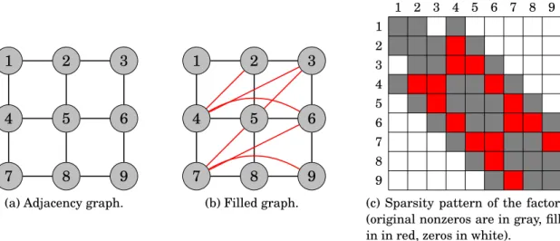
In our illustrative example, the adjacency graph corresponds to the mesh formed by the interior points in Figure1.1, i.e. the graph in Figure1.6a.
1.3.1.2 Symbolic factorization
The symbolic factorization consists in simulating the elimination of the vari-ables that takes place during the numerical factorization to predict the fill-in that will occur. When variable k is eliminated, the update operation
Ai, j← Ai, j− Ai,kAk, j
will fill any entry Ai, j such that both Ai,k and Ak, j are nonzeros, as said before. In terms of graph, this means that when vertex k is eliminated, all its neighbors become interconnected, i.e. a clique is formed. For example, in Figure1.6a, if vertex 1 is eliminated, vertices 2 and 4 are interconnected, i.e. an edge (2,4) must be added (as done in red in Figure1.6b).
After the elimination of variable k, the next step in the numerical factorization is to factorize the trailing submatrix Ak+1:n,k+1:n, and therefore, in the symbolic