Étude de l'efficacité énergétique des navires : développement et application d'une méthode d'analyse

(1)

HAL Id: tel-01001539

https://tel.archives-ouvertes.fr/tel-01001539

Submitted on 4 Jun 2014

HAL is a multi-disciplinary open access archive for the deposit and dissemination of sci-entific research documents, whether they are pub-lished or not. The documents may come from teaching and research institutions in France or abroad, or from public or private research centers.

L’archive ouverte pluridisciplinaire HAL, est destinée au dépôt et à la diffusion de documents scientifiques de niveau recherche, publiés ou non, émanant des établissements d’enseignement et de recherche français ou étrangers, des laboratoires publics ou privés.

Étude de l’eﬀicacité énergétique des navires :

développement et application d’une méthode d’analyse

Pierre Marty

To cite this version:

Pierre Marty. Étude de l’eﬀicacité énergétique des navires : développement et application d’une méthode d’analyse. Thermique [physics.class-ph]. Ecole Centrale de Nantes (ECN), 2014. Français. �tel-01001539�

(2)

Pierre MARTY

Mémoire présenté en vue de l’obtention du

grade de Docteur de l’École Centrale de Nantes

sous le label de L’Université Nantes Angers Le Mans

École Doctorale : Sciences Pour l’Ingénieur Géosciences et Architecture Discipline : Énergétique, Thermique et Combustion

Unité de recherche : Laboratoire de recherche en Hydrodynamique, Énergétique et Environnement Atmosphérique

Soutenue le 16 mai 2014

Ship energy efficiency study: development and

application of an analysis method

---

Étude de l'efficacité énergétique des navires :

développement et application d'une méthode

d'analyse

JURY

Président : Jean-Yves BILLARD, Professeur des Universités, École Navale

Rapporteurs : Georges DESCOMBES, Professeur des Universités, Conservatoire National des Arts et Métiers Patrick SÉBASTIAN, Maitre de Conférences HDR, Université de Bordeaux

Examinateurs : Philippe CORRIGNAN, Docteur, Bureau Veritas

Raphaël CHENOUARD, Maitre de Conférences, École Centrale de Nantes

Invité(s) : Pierre-Yves LARRIEU, Professeur de l’Enseignement Maritime

Directeur de Thèse : Jean-François HÉTET, Professeur des Universités, École Centrale de Nantes

(3)

(4)

Abstract

The shipping industry is facing three major challenges: climate change, increasing bunker fuel price and tightening international rules on pollution and CO2 emissions. All these challenges can be met by reducing fuel consumption. The energy efficiency of shipping is already very good in comparison with other means of transportation but can still be and must be improved. There exist many technical and operational solutions to that extent. But assessing their true and final impact on fuel consumption is far from easy as ships are complex systems. A first holistic and energetic modelling approach tries to deal with this issue. Based on the first law of thermodynamics, it has made it possible to model a complete and modern cruise carrier. Its fuel consumption and corresponding atmospheric emissions were calculated with a good level of accuracy. The model has also proven to very useful at comparing design alternatives hence showing its capacity to evaluate energy efficiency solutions. A second approach completes the first one. Based this time on the second law, including the concept of exergy, it offers a more detailed and physical description of ships. It can precisely assess energy savings, including the part of thermal energy convertible into work. This innovative approach has required new model developments, including a new model of diesel engine, based on the mean value approach, capable of calculating the complete thermal balance for any engine operating point.

(5)

(6)

Résumé

Le transport maritime fait face à trois défis majeurs : le dérèglement climatique, l’augmentation du cours du baril et le durcissement des normes internationales en termes de pollutions et d’émissions de CO2. Ce triple challenge peut être relevé en

réduisant la consommation de fioul. L’efficacité énergétique des navires est déjà très bonne en comparaison avec les autres moyens de transport mais elle peut et doit encore progresser. Il existe à cet effet de multiples solutions techniques et opérationnelles. Mais évaluer leur impact réel sur les économies finales n’est pas toujours chose aisée étant donné la complexité des navires. Une première approche globale de modélisation énergétique du navire tente de répondre à cette problématique. Basée sur le premier principe de la thermodynamique, cette approche a permis de modéliser un paquebot. La consommation de fioul et les émissions associées ont été calculées avec un niveau d’exactitude satisfaisant. Le modèle s’est de plus montré très utile dans la comparaison d’alternatives de conception, illustrant ainsi sa capacité à évaluer les solutions d’économie d’énergie. Une deuxième approche vient compléter la première. Basée cette fois-ci sur le second principe et notamment sur le concept d’exergie, cette approche propose une description plus détaillée et physique du navire. Elle permet d’évaluer précisément les gains d’énergie possibles et en particulier la part convertible en travail mécanique. Cette approche novatrice a nécessité le développement de nouveaux modèles et notamment un nouveau modèle de moteur diesel basé sur l’approche moyenne et qui permet de calculer la balance thermique complète et ce sur tout le champ moteur.

Mots clés : Transport maritime ; Modélisation énergétique ; Exergie ; Modelica ; Efficacité énergétique ; Modélisation moteur diesel

(7)

(8)

ACKNOWLEDGMENTS

This doctorate degree started in May 2011 and finished in May 2014. It took place in Nantes (France) where I divided my time between my company, Bureau Veritas and my laboratories at the École Centrale de Nantes. I could not have achieved this work without the help of people from both these two organizations.

First of all, I would like to express my deepest gratitude to Doctor Philippe Corrignan, who offered me this thesis work. Thank you for your careful attention, your professional skills and challenging remarks. Thank you also for providing me with such fantastic working conditions.

I am also extremely grateful towards Professor Jean-François Hétet, my supervisor. Thank you for your kind patience and sorry for being so “tenacious”.

Very big thanks also to Professor Raphaël Chenouard, my co-supervisor, who patiently explained to me systemics and modelling theories.

I also owe a great debt of gratitude to Professor Pierre-Yves Larrieu for sharing with me his immense and gripping knowledge on ships.

I would like to thank also Professor Jean-Yves Billard, Professor Georges Descombes and Professor Patrick Sébastian for carefully reading my thesis and doing me the honour of being members of my jury.

My special thanks go to Antoine Rogeau, engineer student at the École Centrale de Nantes, who offered me his help when I needed it most.

I am also very grateful to Antoine Gondet, from STX France, for his collaboration in the IMDC paper and cruise ship modelling.

I also would like to thank Pierre Madoz for kindly sharing his knowledge on electrical networks with me. I wish to thank Cédric Brun, for his help on Python.

I would like to express my many thanks towards all my colleagues at Bureau Veritas and Centrale Nantes for their help, kindness and friendship.

Finally, I wish to thank my family and my lovely wife for their unconditional support and encouragement throughout my study.

(9)

(10)

LIST OF FIGURES

Figure 1: Atmospheric carbon dioxide concentrations ...24

Figure 2: Global average temperature change ...25

Figure 3: Emissions of CO2 from shipping compared with global total emissions ...26

Figure 4: Typical range of CO2 efficiencies of ships compared with rail and road transport ...26

Figure 5: Trajectories of the CO2 emissions from international shipping ...27

Figure 6: Crude oil prices trends since 1860 ...28

Figure 7: Oil consumption in thousand barrels per day since 1965 ...29

Figure 1.1: Illustration of reversible and irreversible processes ...39

Figure 1.2: Schematic diagram showing energy, exergy and anergy flows through a closed system transformation ...40

Figure 1.3. Exergetic content of thermal heat ...43

Figure 1.4: Schematic diagram of 66 MW unit of Zarqua’s (Jordan) power plant...45

Figure 1.5: Sankey diagram representing the energetic (a) and exergetic (b) balance of the coal-fired Nanticoke Generating Station in Ontario ...47

Figure 2.1: Basic example of code structure in Modelica ...68

Figure 2.2: Block architecture of Modelica ...70

Figure 2.3: Translation stages from Modelica code to executing simulation ...70

Figure 3.1: SEECAT's diagram view of the modelled cruise vessel ...77

Figure 3.2: Black-box type representation of a diesel engine ...78

Figure 3.3: BSFC map and curve of a Wärtsilä 46 engine ...79

Figure 3.4: Black-box type representation of an electric motor or alternator ...80

Figure 3.5: Black-box type representation of a waste heat recovery boiler ...82

Figure 3.6: Black-box type representation of an oil-fired boiler ...82

Figure 3.7: Black-box type representation of a distiller ...83

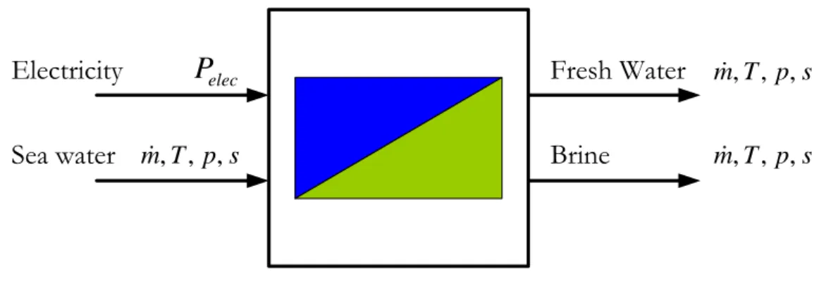
Figure 3.8: Black-box type representation of a reverse osmosis fresh water production unit ...85

Figure 3.9: Black-box type representation of a conditioning system ...86

Figure 3.10: Black-box type representation of the ship’s hydrodynamics ...87

Figure 3.11: Map presenting the route followed by the ship during the four cruises ...89

Figure 3.12: Total instantaneous fuel consumption during the first cruise ...91

Figure 3.13: Total instantaneous electrical production during the first cruise ...92

Figure 3.14: Instantaneous electrical consumption by propulsion motors during the first cruise ...92

Figure 3.15: Instantaneous electrical consumption by other electrical consumers during the first cruise ...94

Figure 3.16: Electrical balance for cruise 1 according to simulation ...95

Figure 3.17: Fuel consumption comparison between the four cruises ...96

Figure 3.18: ASFC comparison between the four cruises...97

Figure 3.19: Electrical consumption comparison between the four cruises ...97

Figure 3.20: Speed profile of a typical 7 days cruise ...99

Figure 3.21: Ship's thermal balance, in winter conditions, without AHRP system ... 102

Figure 3.22: Ship's thermal balance, in winter conditions, with AHRP system ... 102

Figure 4.1: CPP and FPP curves for engine A ... 110

(13)

Figure 4.3: Diesel engine thermal balance presentation, displaying energy inputs and outputs ... 118

Figure 4.4 : Global architecture of the Diesel engine mean value model... 123

Figure 4.5: 3D visualization and contour visualisation of mass flow interpolation ... 131

Figure 4.6: 3D visualisation and contour visualisation of efficiency interpolation ... 133

Figure 4.7: 3D visualisation and contour visualisation of water cooling power interpolation... 134

Figure 4.8: 3D visualisation and contour visualisation of lubrication oil cooling power interpolation ... 136

Figure 4.9: Graphical interface of the SEECAT mean value model of engine A ... 138

Figure 4.10: Brake specific fuel consumption values along the propeller curve ... 139

Figure 4.11: Engine combustion heat values along the propeller curve ... 139

Figure 4.12: Engine jacket water cooling heat values along the propeller curve ... 139

Figure 4.13: Engine lubrication oil cooling heat values along the propeller curve ... 139

Figure 4.14: Scavenge air cooling heat values along the propeller curve... 140

Figure 4.15: Exhaust gas heat (after turbine) values along the propeller curve... 140

Figure 4.16: Exhaust mass flow values along the propeller curve ... 141

Figure 4.17: Exhaust gas (after turbine) temperature values along the propeller curve ... 141

Figure 4.18: Engine operating diagram ... 142

Figure 4.19: BSFC map built using the sensitivity analysis data ... 143

Figure 4.20: Scavenge air cooling heat map built using the sensitivity analysis data ... 143

Figure 4.21: Engine lubrication oil cooling heat map built using the sensitivity analysis data ... 143

Figure 4.22: Engine jacket water cooling heat map built using the sensitivity analysis data ... 143

Figure 4.23: Exhaust mass flow map built using the sensitivity analysis data ... 144

Figure 4.24: Exhaust gas temperature map built using the sensitivity analysis data ... 144

Figure 5.1: Schematic representation of an engine cooling system under the new "fluid circuit" approach ... 152

Figure 5.2 Schematic representation of an engine cooling system under the previous "energy flow" approach ... 152

Figure 5.3: Absolute output energy balance of engine A ... 157

Figure 5.4: Relative output energy balance of engine A ... 157

Figure 5.5: Absolute output exergy balance of engine A ... 158

Figure 5.6: Relative output exergy balance of engine A ... 158

Figure 5.7: SEECAT model of engine A and its cooling and WHR circuit ... 159

Figure 5.8: Energy (a) and exergy (b) Sankey diagrams of engine A with its cooling and exhaust circuits ... 163

Figure A.1: Ship diagram legend ... 176

Figure A.2: Main engine fuel oil supply diagram ... 177

Figure A.3: Main engine lubrication circuit diagram ... 179

Figure A.4: Main engine exhaust and inlet circuits ... 181

Figure A.5: Diesel generator diagram ... 182

Figure A.6: Shaft generator diagram... 184

Figure A.7: Steam turbo-alternator diagram ... 185

Figure A.8: Gas turbine diagram ... 187

Figure A.9: Electric distribution diagram ... 188

Figure A.10: Sea water circuit diagram ... 191

Figure A.11: Fresh water generator diagram ... 193

Figure A.12: Reverse osmosis unit diagram ... 195

Figure A.13: Fresh water distribution circuit ... 196

Figure A.14: Fresh Water Cooling System diagram ... 198

Figure A.15: Fuel circuit diagram ... 199

(14)

Figure A.17: Oil-fired boiler and steam circuit diagram ... 202

Figure A.18: Oil-fired and waste heat recovery boilers diagram ... 204

Figure A.19: Condenser diagram ... 205

Figure A.20: Oil-fired boiler burners diagram ... 207

Figure A.21: HVAC system diagram ... 208

Figure B.1: (PV) and (TS) diagrams of the Diesel cycle ... 211

Figure B.2: Typical cycle for a real diesel engine ... 212

(15)

(16)

LIST OF TABLES

Table 1: Assessment of potential reductions of CO2 emissions from shipping by using known

technology and practices, according to IMO [6] ... 32

Table 1.1: Comparison of energy and exergy ...42

Table 1.2: Exergy analysis of Zarqua’s power plant ...46

Table 2.1: Comparison between a complicated and a complex problem ...54

Table 2.2: Comparison between analytical and systemic approach ...56

Table 2.3: Comparison between analytical and empirical approach ...59

Table 2.4: Comparison between causal and acausal models ...60

Table 2.5: Comparison between the "Energy flow" approach and the "Fluid circuit" approach ...66

Table 2.6: Potential and flow variables for different physical fields in Modelica ...69

Table 2.7: Content of Modelica Standard Library ...71

Table 3.1: Main characteristics of cruises selected for verification ...89

Table 3.2: STX and SEECAT data comparison for the first cruise ...90

Table 3.3: Design alternatives’ fuel consumption comparison in summer conditions ... 100

Table 3.4: Design alternatives’ emissions comparison in summer conditions ... 100

Table 3.5: Design alternatives’ fuel consumption comparison in winter conditions ... 100

Table 3.6: Design alternatives’ emissions comparison in winter conditions ... 101

Table 4.1: Comparison of specifications and requirements among various diesel engines modelling approaches ... 115

Table 4.2: Engine thermal balance: list of output and input power flows and corresponding equations ... 118

Table 4.3: Comparison between two complete thermal balances of engine A... 121

Table 4.4: Distribution of heat losses (except radiation) for thermal balances A1 and A2 ... 122

Table 5.1: Energetic and exergetic content of engine A output power ... 156

Table 5.2: Standard simulation parameters... 160

(17)

(18)

NOMENCLATURE

Anergy production or exergy destruction [ J ]

Specific anergy [ J/kg]

Heat capacity [ J∙K-1_]

Specific heat capacity [ J∙K-1_∙kg-1_]

Exergy [ J ] Specific exergy [ J/kg] Enthalpy [ J ] Specific enthalpy [ J/kg] ̇ Mass flow [kg/s] Number - Power [W] Pressure [Pa] Pressure ratio - Heat [ J ]

̇ Heat transfer rate [W]

Specific perfect gas constant [ J∙K-1_∙kg-1_]

Entropy [ J∙K-1_] Specific entropy (J.K-1_.kg-1₎ _{[ J∙K}-1_∙kg-1_] Temperature (K) [K] V Volume [m3_] Work [ J ] ̇ Work rate [W]

(19)

 Greek letters:

Adiabatic index -

Specific chemical exergy of a fuel [ J/kg]

Effectiveness -

Efficiency -

Carnot factor (1-Ta/T) -

Air-fuel equivalence ratio or air excess ratio -

Torque [N ∙ m]

Rotary velocity [rad/s]

(20)

 Subscript:

Ambient

Brake

Calorific

Chemical

Cycle per second

Delivered

Output quantity across port e

Electric Energy Exhaust receiver Exergy Exhaust External Frigorific Fresh water

Input quantity across port i – Indicted

Internal Mechanical At constant pressure Post-combustion Propeller Reference Isentropic Stoichiometric Sea water Total Thermomechanical / thermal

(21)

 Acronyms and abbreviations:

AHRP Advanced Heat Recovery Plant

ASFC Average Specific Fuel Consumption

BMEP Brake mean effective pressure (Pa) BSFC Brake specific fuel consumption (g/kWh)

CFD Computational Fluid Dynamic

COP Coefficient Of Performance

CPP Controllable pitch propeller

CR Compression ratio

DG Diesel Generator

DO Diesel oil

EEDI Energy Efficiency Design Index

EEOI Energy Efficiency Operational Index

FLT First law of thermodynamics

FMEP Friction mean effective pressure (Pa)

FO Fuel oil

FPP Fixed pitch propeller

FWG Fresh Water Generator

GDP Gross domestic product

GHG Greenhouse gases

HFO Heavy fuel oil

HHV Higher heating value (J/kg)

HT High Temperature

HVAC Heating Ventilation and Air Conditioning IMEP Indicated mean effective pressure (Pa) IMO International Maritime Organization

IPCC Intergovernmental Panel on Climate Change

LFO Light fuel oil

LHV Lower heating value (J/kg)

LNG Liquefied natural gas

LO Lubrication oil

LT Low Temperature

Lub. Lubricating

MCR Maximum continuous rating (engine power)

MDO Marine Diesel oil

MVEM Mean Value Engine Model

(22)

OECD Organisation for Economic Co-operation and Development

OFB Oil Fired Boiler

ORC Organic Rankine Cycle

PMS Power management system of the ship’s electrical power plant

RCP Representative Concentration Pathways

ROPU Reverse osmosis production unit

SAC Scavenge air cooler

SEECAT Ship Energy Efficiency Calculation and Analysis Tool SEEMP Ship Energy Efficiency Management Plan

SLT Second law of thermodynamics

SOX Sulphur oxides

SRES Special Report on Emissions Scenarios

(23)

(24)

THESIS ORGANISATION

The present document is mainly composed of an introduction, five chapters, a general conclusion and appendices. The two first chapters are bibliographic reviews and theoretical presentations concerning respectively the concept of exergy and modelling techniques applied to energetic systems. The last three present the development work.

The Introduction presents the environmental, economic and regulatory context and defines the study objectives.

Chapter 1 “Ship Energy Efficiency” starts by presenting the fundamental definitions, equations and notions relative to Energy and Exergy. A bibliographic review of energy and exergy analysis methods is then presented.

In Chapter 2 “Ship Energy Modelling”, a first part presents the theory of systemics. It is followed by a presentation of an energy modelling method and the Modelica modelling language.

Chapter 3 “Holistic Modelling” presents a first ship energy modelling approach based on power conversion. This approach is then applied to a real ship for which sea measurement data were available. The model produced is presented and its validation discussed. The use of this model is finally illustrated by comparing different ship design alternatives.

In Chapter 4 “Engine Modelling”, a limitation of the first ship energy modelling approach is answered by developing a new engine model. The objectives and constraints of the model are first discussed. The data available is then presented. The best suited modelling approach is selected based on a bibliographic review. The data available is then analysed and cleaned. The structure of the model and its equations are presented. Finally, the validity of the model is discussed.

Chapter 5 “Fluid Circuit & Exergy Modelling” introduces a second level approach called “circuit fluid” approach. This approach makes it possible to use the exergy analysis. It is applied to a ship main engine and its cooling and exhausts circuits. A set of ideas for energy and exergy saving is proposed.

A general Conclusion closes the main corpus of the thesis and proposes new work perspectives.

The Appendices contain in particular an extensive description of all the main energy circuits on board ships.

(25)

(26)

INTRODUCTION

“There is too much fossil energy on this planet to count on its limitation to save the climate but there is not enough of it to count on its abundance to restart the European economy”

Jean Marc Jancovici [1]

INTRODUCTION ... 23

ENVIRONMENTAL CONTEXT ... 24

ECONOMIC CONTEXT ... 28 REGULATORY CONTEXT ... 29

(27)

24 Introduction

E

NVIRONMENTAL CONTEXT

In September 2013, the Intergovernmental Panel on Climate Change (IPCC) has released the first part of its fifth assessment report, The Physical Science Basis [2]. This report, written by more than two hundred authors*_{, reviewed by over a thousand experts compiles and synthesises}†_{peer reviewed publications of} thousands of scientists around the world‡_{. It offers the latest state of the art knowledge on climate change.} This report is accompanied by a 33 pages long summary for policymakers [3]. This summary highlights the main conclusions of the full report. The most relevant conclusions of this report are presented below. This report reminds us that climate change is a reality and that its consequences are already measureable:

“Warming of the climate system is unequivocal, and since the 1950s, many of the observed changes are unprecedented over decades to millennia. The atmosphere and ocean have warmed, the amounts of snow and ice have diminished, sea level has risen, and the concentrations of greenhouse gases have increased.”

Furthermore, this report leaves almost no doubt possible concerning the origin of climate change:

“Human influence on the climate system is clear.[...] It is extremely likely§_{that human influence}

has been the dominant cause of the observed warming since the mid-20th century.”

Figure 1: Atmospheric carbon dioxide concentrations measured at the Mauna Loa observatory in ppmv (part per million by volume)

The clearest sign of this “human influence” is the strong increase in carbon dioxide atmospheric concentration which is due mainly to fossil fuel combustion. The Mauna Loa observatory (Hawaii, USA) has continually recorded atmospheric CO2 levels since 1956. Its data is publically available and serves as a reference in the scientific world. Between 1956 and 2012, atmospheric CO2 concentration has increased

*_{209 lead authors, 50 review editors and over 600 hundred contributing authors} †_{The report is nevertheless more 2000 pages long}

‡_{Over 2 million gigabytes of numerical data from climate model simulations and over 9200 scientific publications} cited §_{95–100% probability} 290 310 330 350 370 390 410 1950 1960 1970 1980 1990 2000 2010 2020 C ar bo n dio xy de c on ce ntra tio n [p pmv]

(28)

Environmental context 25

by over 25%. This increase is continuous and getting stronger with time (see Figure 1). More globally, the IPCC reports that:

“The atmospheric concentrations of carbon dioxide, methane, and nitrous oxide have increased to levels unprecedented in at least the last 800,000 years. Carbon dioxide concentrations have increased by 40% since pre-industrial times, primarily from fossil fuel emissions and secondarily from net land use change emissions. The ocean has absorbed about 30% of the emitted anthropogenic carbon dioxide, causing ocean acidification”

Figure 2: Global average temperature change. The black curve corresponds to the modelled historical temperature, the red one corresponds to scenario RCP8.5 and the blue one to scenario RCP2.6. These curves are obtained by averaging results of various models (more than 30 each). The shadings are a measure of uncertainty [3].

Historical emissions of greenhouse gases (GHG) have already modified the climate and will continue to do so for decades even if these emissions were to stop completely tomorrow. The damages done is almost irreversible but may still be manageable. Nevertheless, GHG emissions are due to continue and hence climate change worsen. The future evolution of the climate has been assessed by Van Vuuren et al [4] according to different scenarios. These scenarios are based on different hypothesis such as world population growth, world GDP*_{growth, energy consumption growth and the evolution of the type of} energy consumed (solar, wind, geothermal, hydraulic, bio-fuels, nuclear, gas, oil or coal). Climate models are used to evaluate the increase of global temperature following these different scenarios. Four scenarios called RCP, for Representative Concentration Pathways, were built. The future evolution of global average temperature is presented following two of these scenarios: the most optimistic and the most pessimistic ones (see Figure 2). For the sake of brevity, only the evolution of temperature is presented, nevertheless, global change is not limited to temperature change. The evolution of global ocean surface pH, sea levels, sea ice extent, levels of precipitation are other crucial points. For more details, interested readers can refer to the work already cited.

Scenario RCP2.6 is an optimistic scenario. The global mean temperature increase in 2081-2100 compared to 1986-2005 is likely to be in a range of “only” 0.3 °C to 1.7 °C. The temperature should settle down and

(29)

26 Introduction

even decrease a little by 2100. Following this path would require great emission reduction efforts. On the other hand, scenario RCP8.5 is a pessimistic scenario in which emissions are not handled and continue to increase strongly. In such case, the temperature increase would be in a range of 2.6 °C to 4.8 °C. Moreover, the temperature would tend to continue increasing.

If these variations can seem small, it must be reminded that an average surface temperature difference of only 5 °C separates us from the previous glacial age and that the temperature evolution since 1950 is the fastest ever recorded [5]. The consequences on the environment and hence humanity could be dramatic. Following either of these two paths is of crucial importance. It is a choice that belongs to every government, company and citizen.

The shipping industry can be seen as a small contributor to climate change. In 2009, the IMO*_{published a} report where the contribution of the total shipping industry†_{to the world global emissions was assessed to} correspond to “only” 3.3% (see Figure 3) [6]. The figure is quite impressive bearing in mind that shipping is responsible for the transportation of 80% in volume of total merchandise [7]. Shipping is in fact a very efficient means of transportation. When the CO2 emissions are related to the tonne of merchandise and the distance travelled, shipping is found to be more efficient than road transport in every case and more efficient than rail transport in a majority of cases (see Figure 4).

Figure 3: Emissions of CO2 from shipping compared with

global total emissions. Shipping is estimated to have emitted 1,046 million tonnes of CO2 in 2007, which

corresponds to 3.3% of the global emissions during 2007 [6].

Figure 4: Typical range of CO2 efficiencies of ships

compared with rail and road transport. Air freight is not presented on this figure but its CO2 efficiency has been

calculated to be in a range of 435 to 1800 g CO2/tonne*km [6].

*_{International Maritime Organization: http://www.imo.org/} †_{International shipping plus domestic shipping and fishing}

Other transport (road) 21.3% Rail 0.5% International

aviation 1.9% Total shipping 3.3%

Electricity and heat production 35.0% Other energy industries 4.6% Other 15% Manufacturing industries and construction 18.2% 0 50 100 150 200 Crude LNG General cargo Reefer Chemical Bulk Container LPG Product Ro-Ro/Vehicle Rail Road g CO2/tonne*km

(30)

Environmental context 27

Nevertheless, efforts must be made to reduce CO2 emissions. Historically, there always has been a strong link between economic growth and seaborne trade. Yet the world GDP growth was of 3.2% in 2012, 2.9% in 2013 and it is projected to be of 3.6% in 2014 [8]. If the world economy increases at a rate of 3% for the next 25 years then the world GDP will have more than doubled. GHG emissions due to shipping could hence increase in similar proportions. The future evolution of CO2 emissions from international shipping has been assessed by the IMO based on SRES*_{scenarios from the 2007 IPCC report [5]. The} results are presented in Figure 5.

Figure 5: Trajectories of the CO2 emissions from international shipping (million tonnes CO2/year). The coloured lines

correspond to mean evolution according to IPCC 2007 report SRES scenarios [5]. The dashed lines correspond to the most optimistic and pessimistic scenarios [6].

The calculated emissions from shipping in 2050 vary over a wide range: from a multiplication by more than 7 in the worst case scenario to a small decrease in the best one. Nevertheless, the mean values of each scenario follow similar trends (indicating by the way a good reliability) were carbon dioxide emissions may grow by a factor 2 to 3 by 2050.

Proactive actions must be taken to avoid this foreseeable future. Such actions already exist or are in development. The IMO has estimated that technical and operational measures could possibly reduce GHG emissions by 25% to 75% compared to current levels (see section “Doctorate objectives” below). Some of these measures are cost-effective; others are not and will have to be supported by new binding policies to be put in place. Assessing accurately the fuel reduction and hence GHG emissions reduction of any measure is therefore essential for ship owners who will have to choose the best solution for the least investment. This is especially true given the constraint of high fuel prices.

(31)

28 Introduction

E

CONOMIC CONTEXT

The maritime industry is very dependent on fuel price. The overwhelming majority of commercial ships use fossil fuel energy to navigate (heavy fuel oil and diesel oil in vast majority and a bit of gas or coal) and fuel cost has become the second or first item in operational expenditures. This situation is not on the verge of changing favourably, as fuel prices have historically almost always increased (see Figure 6) and are physically bound to continue. The main reasons for that are:

 The limited resource: even if new stocks are discovered frequently the resource is physically limited. Certain regions have certainly already reached or passed their pick oil such as northern Europe.

 The increasing difficulty to extract oil: oil companies have to dig deeper and deeper to extract oil, increasing further the price in addition to increasing the risk of environmental pollutions.

 The decreasing quality of the extracted oil: as conventional oils become less available, oil companies have invested in the production of oil from new sources such as oil sands, oil shale and heavy crude oil. These unconventional sources require more energy and therefore more money to extract and transform.

 The increasing demand: even if the oil consumption of OECD*_{countries has settled down or even} decreased over the last decade, the world demand continues to increase strongly, mainly due to the increasing world population and its increasing living standard. This is particularly true for Asia with China and India (see Figure 7).

Figure 6: Crude oil prices trends since 1860 [9]

This long term trend towards high fuel prices is certainly a strong incentive to fuel consumption reduction. But it is not strong enough to guarantee the best fuel consumption reduction possible. Additional regulatory constraints are therefore necessary.

*_{Organisation for Economic Co-operation and Development: list of 34 “developed” countries mainly including UE} countries, North America countries, Turkey, Chili, Australia, New-Zealand, Japan and South-Korea.

20 40 60 80 100 120 1 860 1 880 1 900 1 920 1 940 1 960 1 980 2 000 2 020 Crude oil prices [US $/barrel]

(32)

Regulatory context 29

Figure 7: Oil consumption in thousand barrels per day since 1965 [9]

R

EGULATORY CONTEXT

The strong scientific evidence for climate change and its major contributor, anthropogenic emissions, have led policy makers to take direct actions to reduce CO2 emissions in the recent years: Kyoto protocol (1997), European Union reduction plan by 2020. Despite the fact that maritime transportation is the most carbon efficient way of motorized transportation, seaborne emission regulations have not been overlooked. The IMO has strengthened its regulations on NOX and SOX emissions and introduced CO2 regulation with tools such as EEDI, EEOI and SEEMP.

 Energy Efficiency Design Index (EEDI)

The EEDI assesses the CO2 performance of the ship design. It is evaluated at building stage and verified during sea trials [10]. The EEDI expresses a ratio between the environmental impact of shipping and the benefit enjoyed by the community from shipping. Equation (1) presents a simplified version of EEDI.

₍₁₎

The real equation of EEDI is rather complicated and takes into account energy consumers as well as specific features or needs such as energy recovery systems, the use of low-carbon fuels, the performance of ship in waves or the need for ice strengthening [11]. The EEDI is expressed in grams of CO2 per capacity-mile, where “capacity” refers to the type of cargo the ship is designed to carry. For most ships, the “capacity” is expressed in deadweight tonnage*_.

*_{The Deadweight tonnage is a measure (in tonnes) of how much weight a ship can safely carry. It is the sum of the} weights of cargo, fuel, fresh water, ballast water, provisions, passengers, and crew.

0 10 000 20 000 30 000 40 000 50 000 60 000 70 000 80 000 90 000 100 000 1965 1970 1975 1980 1985 1990 1995 2000 2005 2010

Oil consumption in thousand barrels per day

Total Asia Pacific Total Africa Total Middle East Total Europe & Eurasia Total S. & Cent. America Total North America

(33)

30 Introduction

The EEDI resolution [12] came into force on the 1st_{of January 2013. It applies to most ships types (bulk} carrier, gas tanker, tanker, container ship, general cargo ship, refrigerated cargo, ro-ros, passenger ships) with the exception of working ships (offshore vessels, dredgers, supply vessels, tugs) and ships with specific propulsion systems (diesel-electric, turbine, hybrid). Ship with a gross tonnage*_{lower than 400 are} also exempted. All new ships concerned by the resolution must show an EEDI value lower than a regulatory baseline, otherwise the ship will not be allowed to navigate. The baseline depends on the ship type and is a decreasing function of the ship size. Moreover, this baseline is planned to reduce over the years, therefore increasing the incentive for energy efficient ship designs.

EEDI is a fixed performance indicator calculated for one operating point. It is not suited for energy efficiency monitoring in service. EEOI is more adapted for that purpose.

 Energy Efficiency Operational Index (EEOI)

The basic principle of EEOI is similar to EEDI, it assesses the CO2 performance of a ship. But unlike EEDI, EEOI is calculated for each leg of a voyage using the following formula [13]:

∑

(2)

Where:

 is the fuel type;

 is the mass of consumed fuel ;

 is the fuel mass to CO2 mass conversion factor for fuel ;

 is the cargo carried (tonnes) or work done (number of TEU†_{or passengers) or gross tonnes} for passenger ships; and

 is the distance in nautical miles corresponding to the cargo carried or the work done.

The EEOI is expressed in the same unit as EEDI, that is to say in grams of CO2 per capacity-mile. It also measures the ship energy efficiency in service.

For the moment EEOI monitoring is not mandatory. But it can be used, on a voluntary basis, to build the SEEMP.

 Ship Energy Efficiency Management Plan (SEEMP)

To help shipping companies manage the CO2 efficiency of their fleet, the IMO has developed and defined a new tool: the SEEMP [14]. This tool is put into practice by following four phases that form a cycle:

 Planning: in this phase, the main actions of the SEEMP are to assess current ship energy usage, to identify energy-saving measures that have already been implemented and evaluate their effectiveness and to list future potential improvements. Of course, these measures depend on the ship type, size and operation. To insure the best implementation possible, several additional actions are recommended:

*_{Gross tonnage is a unitless index related to a ship's overall internal volume. It is not a physical measure but rather} an administrative one. It is used notably for ship's manning regulations, safety rules, registration fees, and port dues. †_{Twenty-foot Equivalent Unit (TEU): unit used to describe the capacity of container ships based on the volume of a} 20-foot-long (6.1 m) intermodal container.

(34)

Doctorate objectives 31

involve all ship stakeholders (ship repair yards, ship-owners, operators, charterers, cargo owners, ports and traffic management services), provide crew training and set emission reduction goals.

 Implementation: the actions identified in the previous phase are implemented.

 Monitoring: the efficiency of these actions should be monitored quantitatively (this can be done using EEOI).

 Self-evaluation and improvement: in this final phase, a critical review of the first three phases is made. The effectiveness of the actions implemented and their implementation are self-evaluated in order to produce relevant feedback for the following improvement cycle.

In the end the SEEMP takes the form of a document. Whilst the presence of this document on board of every ship is mandatory, for now the content of it is overlooked.

The three tools, EEDI, EEOI and SEEMP have been implemented in the MARPOL Annex 6 [15] which is the IMO convention for the Prevention of Pollution From Ships. They constitute a first regulatory step towards increasing ship energy efficiency.

D

OCTORATE OBJECTIVES

The maritime industry is hence facing three challenges: environmental - due to the greenhouse effect and climate change as well as pollutant emissions, economic - due to increasing bunker fuel price, and regulatory - with new laws. All three challenges can be met through one single measure: reducing fuel consumption.

This can be achieved through various measures (see Table 1), such as optimizing hull shape and propeller design to ensure lower propulsion power or improving the efficiency of machinery equipment or systems (for example diesel engines, electrical motors, alternators, boilers, distillers, pumps, turbines, etc.). Reducing fuel consumption can also be achieved by changing the operational cycle such as adopting ship speed reduction (slow steaming). A combination of these techniques and often all of them together are used in new ship design. A new ship may boast a new engine that effectively consumes 5% less fuel. It may also have a new hull that presents 5% less hydrodynamic resistance. But in the end the ship may not consume 9.75%*_{less fuel. This is to do with the complexity of a ship. A ship is composed of many} devices producing and consuming energy and there are many interactions amongst them. For instance reducing speed or hydrodynamic resistance leads to lower mechanical power requirement and hence lower fuel consumption. But it also leads to less thermal energy loss which is often recovered on board for various purposes (for example bunker fuel heating, cabin heating, fresh water production using distillers, sanitary water heating, steam production, etc.). Less thermal energy may lead in certain cases to starting an oil fired boiler and hence increase fuel consumption. This simple theoretical example illustrates the complexity of ships and the fact that calculating energy consumption is neither direct nor obvious.

This thesis offers to meet this complexity and will provide methods and tools to assess correctly means of fuel reduction. In particular, a simulation platform, called SEECAT, will be developed for that goal. The systems approach will help grasp the complex nature of ships and help define the best modelling approach. The exergy concept will allow a better understanding of the different energetic processes at stake as well as determining more accurately the true energy saving potentialities.

(35)

32 Introduction

Moreover, holistic ship energy and exergy modelling are growing topics in the maritime industry and academic world. They nevertheless suffer from a limited literature background. And to that extent, this thesis should constitute an innovative work.

Table 1: Assessment of potential reductions of CO2 emissions from shipping by using known technology and practices,

according to IMO [6]

Saving of CO2/tonne-mile Combined Combined

DESIGN (New ships)

25% to 75%* Concept, speed and capability 2% to 50%*

10% to 50%* Hull and superstructure 2% to 20%

Power and propulsion systems 5% to 15%

Low-carbon fuels 5% to 15%†

Renewable energy 1% to 10%

Exhaust gas CO2 reduction 0% OPERATION (All ships)

Fleet management, logistics & incentives 5% to 50%*

10% to 50%*

Voyage optimization 1% to 10%

Energy management 1% to 10%

†_CO₂_{equivalent, based on the use of LNG}

*_{Reductions at this level would require reductions of operational speed}

Objectifs de la thèse

L’industrie maritime fait donc face à trois défis : le défi environnemental dû aux gaz à effet de serre et au dérèglement climatique, le défi économique dû à l’augmentation continue du prix du fioul et le défi réglementaire dû aux nouvelles lois. C’est trois défis peuvent être relevés grâce à une unique mesure : la réduction de la consommation de fioul.

Cette réduction de consommation peut être obtenue de plusieurs manières (voir tableau 2), telle que l’optimisation de la forme de la carène et des hélices afin de diminuer la puissance propulsive ou l’amélioration du rendement des différents systèmes à bord (par exemple les moteurs diesel, les moteurs électriques, les alternateurs, les chaudières, les bouilleurs, les pompes, les turbines, etc.). La réduction de la consommation peut également être obtenue en agissant sur le profil opérationnel en réduisant par exemple la vitesse. Une combinaison de ces méthodes et souvent toutes ces méthodes à la fois sont utilisées lors de la conception de nouveaux navires. Un nouveau navire peut par exemple avoir des moteurs diesel consommant 5 % de fioul en moins, ainsi qu’une coque réduisant la résistance hydrodynamique de 5 %. Mais à la fin, l’ensemble ne consommera pas nécessairement 9.75 %*_{de fioul en moins. Ceci est dû à la complexité des navires. Les navires sont composés de multiples}

machines produisant et consommant de l’énergie et il peut y avoir des nombreuses interactions entre ces machines. Par exemple, réduire la vitesse du navire ou sa résistance hydrodynamique aura pour effet une moindre demande de puissance mécanique et donc une moindre consommation de fioul des moteurs. Mais cette baisse de la consommation aura pour effet direct une baisse de la puissance thermique disponible, puissance thermique qui est souvent récupérée et qui assure de multiples

(36)

Doctorate objectives 33

besoins (par exemple le chauffage des soutes à combustible pour les tankers et plus généralement le chauffage des cabines, la production d’eau douce grâce aux bouilleurs, la production d’eau chaude sanitaire, la production de vapeur, etc.). Cette baisse de la consommation de fioul des moteurs pourrait ainsi, dans certains cas, entrainer un démarrage des chaudières à bruleurs pour pallier ce manque de puissance thermique et ainsi ré-augmenter la consommation globale de fioul du navire. Ce simple exemple théorique permet d’illustrer la complexité des navires et montre comment le calcul de la consommation énergétique d’un navire n’est ni direct ni évident.

Cette thèse aborde cette complexité et propose des méthodes et des outils afin d’évaluer correctement des solutions pour réduire la consommation des navires. Une plateforme de simulation, appelée SEECAT, sera notamment développée à cet effet. L’approche système permettra de gérer la nature complexe des navires et aidera à définir la meilleure approche de modélisation à suivre. Le concept d’exergie permettra une meilleure compréhension des différents processus énergétiques à l’œuvre et une meilleure évaluation des gains énergétiques potentiels.

De plus, la modélisation énergétique et exergétique globale des navires est un sujet émergent dans le monde de l’industrie maritime et le monde académique. Ce sujet est malheureusement mal documenté dans la littérature spécialisée. Cette thèse se veut donc être une contribution innovante à ce sujet.

Tableau 2: Évaluation des réductions potentielles d’émissions de CO2 du transport maritime en ayant recours à des

pratiques et des technologies connues (selon l’Organisation Maritime Internationale [6])

Économie de CO2/tonne-mile Combinées Combinées

CONCÉPTION (bateau neuf)

25 % à 75 %* Conception, vitesse et capacité 2 % à 50 %*

10 % à 50 %* Coque et superstructure 2 % à 20 %

Puissance et systèmes propulsifs 5 % à 15 % Carburant à faible teneur en carbone 5 % à 15 %† Énergies renouvelables 1 % à 10 % Réduction de CO2 des gaz d’échappement 0 %

OPÉRATION (tous navires)

Gestion de la flotte, logistique et incitations 5 % à 50 %*

10 % à 50 %* Optimisation du routage 1 % à 10 %

Gestion de l’énergie 1 % à 10 % †_{En équivalent CO}₂_{, basé sur l’usage de gaz naturel liquéfié}

(37)

(38)

CHAPTER 1 SHIP ENERGY EFFICIENCY

CHAPTER 1 SHIP ENERGY EFFICIENCY ... 35

1.1 ENERGY AND EXERGY FUNDAMENTALS ... 36

1.1.1 Energy ... 36

1.1.1.1 First law of thermodynamics ... 37 1.1.1.2 Second law of thermodynamics ... 38

1.1.2 Exergy ... 40

1.1.2.1 Definition of exergy ... 40 1.1.2.2 Properties of exergy ... 41 1.1.2.3 Reference environment ... 42 1.1.2.4 Exergy of thermal heat ... 42 1.1.2.5 Exergy loss and exergy destruction ... 43 1.1.2.6 Conclusion concerning exergy ... 44 1.2 ENERGETIC AND EXERGETIC ANALYSIS ... 44

(39)

36 1 Ship Energy Efficiency

Saving energy is the most straightforward and efficient way of reducing carbon dioxide emissions and it can possibly save money. But in order to save energy, it is essential to correctly assess it. That is especially the case for complex systems such as ships where energy exists in many forms (thermal - steam, cooling water or lubrication oil, mechanical - engine shaft rotation or propeller thrust, chemical - fuel and electricity) and undergoes many transformations (combustion, expansion, compression, heating, cooling, etc.). Correctly understanding and representing the complete set of energy flows and transformations on board ships is the first step towards energy saving. To that extent, the concept of exergy will help understanding the different energy processes at stake and the different energy saving potentialities.

In this chapter, the theory fundamentals of energy and exergy will be presented. It will be followed by the presentation of energy and exergy analysis applied to power plants.

Les économies d’énergie sont le moyen le plus simple et le plus direct de réduire les émissions de dioxyde de carbone et permettent éventuellement d’économiser de l’argent. Mais afin d’économiser de l’énergie, il est au préalable nécessaire de correctement la quantifier. Ceci est d’autant plus vrai pour les systèmes complexes tels que les navires où l’énergie existe sous plusieurs formes (sous forme thermique avec la vapeur, l’eau de refroidissement des moteurs et l’huile de lubrification, sous forme mécanique avec le travail de l’arbre moteur ou la poussée de l’hélice, sous forme chimique avec les différents combustibles ou encore sous forme électrique) et subissent de multiples transformations (combustion, détente, compression, chauffage, refroidissement, etc.). Correctement comprendre et représenter ces ensembles de flux d’énergie et de transformations est la première étape vers d’éventuelles économies d’énergie. À cet égard, le concept d’exergie permettra de mieux comprendre les différents processus énergétiques à l’œuvre et de mieux évaluer les possibilités d’économies d’énergie.

Dans ce chapitre, les fondamentaux théoriques de l’énergie et de l’exergie seront présentés. Ils seront suivis d’une présentation sur l’analyse énergétique et exergétique appliquée aux centrales électriques.

1.1 E

NERGY AND EXERGY FUNDAMENTALS

Exergy is a concept that stems from thermodynamics; it is also a physical quantity, similar to energy, measured in Joules or its derivatives. The term was first introduced by a Slovenian scientist, Zoran Rant in 1956 [16]. It is also synonymous with: availability, available energy, exergic energy, essergy, utilizable energy, available useful work, maximum (or minimum) work, maximum (or minimum) work content, reversible work, and ideal work.

To fully understand the concept of exergy, it is necessary to first present the basic rules of thermodynamics. Thermodynamic is the science of energy transfers. It is mainly ruled by two laws: the first law of thermodynamic that states that for any energetic process (except nuclear reactions) energy is conserved; and the second law of thermodynamic that states that not all energetic processes are possible.

1.1.1 Energy

Energy is a physical quantity measured in Joules or its derivatives. It exists in various forms:

 Mechanical energy: it can take several forms, the energy associated with the motion of an object is called kinetic energy, the energy associated with the position of an object is called gravitational potential energy and the energy associated with the force that causes the motion of an object is called work.

 Electrical energy: the potential energy linked to an electrical charge into an electrical field

(40)

1.1 Energy and exergy fundamentals 37

 Radiant energy: it is a combination of the two preceding energies, it is the energy of electromagnetic waves or particle. The most common form of radiant energy is the energy of the sun light. X-rays, γ-rays, ultraviolet and infrared light and also radio and microwaves have radiant energy.

 Chemical energy: potential energy linked to the electronic structure of molecules. Chemical energy is released or gained through chemical reactions. Combustion is a chemical reaction where energy is released, the process of charging a battery is a chemical reaction that consumes energy.

 Nuclear energy: potential energy linked to the cohesion of the nucleons inside an atom’s nucleus. This energy can be released via nuclear reactions such as fission and fusion.

 Heat energy: the energy transferred from a body to another via a thermal process (convection, conduction or radiation)

In thermodynamics, these different forms of energy can be classified into two groups: macroscopic and microscopic energy. Macroscopic forms of energy are linked to the overall system such as the kinetic and potential energy of the system. The microscopic form of energy is the energy linked to the molecular structure inside the system. The molecules inside the system have also kinetic and potential energy. The microscopic kinetic energy is due to the motion of each particle inside the system (translation, rotation, vibration). The microscopic potential energy includes chemical, nuclear, electric, magnetic and gravitational potential energy. The sum of all microscopic energies is called internal energy.

Therefore, all systems have multiple forms of energy and measuring or calculating each one of them can be very difficult and time consuming. Assessing the absolute energy of a system is therefore almost impossible. On the contrary, energy variations through transformations are much easier to access. Here is a list of transformation examples:

 A combustion process transforms the chemical energy of fuel into heat

 A heat engine transforms heat into mechanical force

 A wind turbine transforms the kinetic energy of wind into mechanical energy

 An alternator transforms mechanical energy into electricity

 An electrical engine transforms electricity into mechanical energy

 A solar panel transforms solar energy (electromagnetic energy of the sun light) into electricity

 A power dam transforms the potential energy of water into mechanical energy

 A electrical battery can transform chemical energy into electricity and vice versa

 The photosynthesis process is used by plants to convert the light’s energy into chemical energy

1.1.1.1 First law of thermodynamics

The first law of thermodynamics states that energy can neither be created, nor destroyed, but can only change form. This law is the law of the conservation of energy. An equivalent statement is that the energy of an isolated system is constant.

It is necessary to introduce the following definitions:

 Open system: a system which can exchange energy and matter with its surrounding, e.g., turbines, pumps, internal combustion engines.

 Closed system: a system which can exchange only energy (no matter) with its surrounding, e.g., cooling loops, refrigerating circuit, water circuits in Rankine cycles.

 Isolated system: a system which cannot exchange, neither energy nor matter with its surrounding. The only true isolated system known is the universe as a whole.

(41)

Given the following variables:

 : work exchanged between the system and its surrounding,

 : thermal energy (or heat) exchanged between the system and its surrounding,

 : electrical energy exchanged between the system and its surrounding,

 : internal energy variation,

 : external potential energy variation,

 : external kinetic energy variation,

 : electric energy variation,

the first law of thermodynamics can be written as:

_(1.1)

The left part of equation (1.1) corresponds to energy exchanged between the system and the environment. The right part corresponds to energy variation in the system itself. Both parts of the equation provide space for possible additional energies such as light, nuclear or chemical energies. For a thermomechanical system, that is to say a system where only mechanical and thermal energy variations and exchange occur, equation (1.1) can be simplified into:

_(1.2)

If a motionless system is considered: and and therefore, equation (1.2) becomes:

_(1.3)

The first law of thermodynamics is the law of energy equivalence or energy conservation. According to this law, energy must be conserved throughout any energetic process. Spontaneous (natural) processes have a preferred direction of evolution. For example heat always flows from hot to cold reservoirs and never the opposite unless work is provided*_{. This restriction is due to the second law of thermodynamics.}

1.1.1.2 Second law of thermodynamics

Sadi Carnot is credited to be the first to formulate the second law of thermodynamics. Modern statements of the second law use the concept of entropy . Entropy is a state function which expresses a measure of disorder or randomness and has for unit Joules per Kelvin (J/K). The entropy of a thermodynamic system can change under the influence of internal entropy creation ( ) and entropy exchange with the surrounding ( ):

_(1.4)

*_{According to the first law only, exotic energetic process could occur: a ship could for example cool down the sea to} navigate, which is of course impossible

(42)

Each time the system receives or gives away heat to its surrounding (environment or thermal sources) it receives or gives away entropy:

_(1.5)

Where is the temperature of the surrounding.

The creation of internal entropy depends on the quality of the transformation:

 for a reversible process (ideal process)

 for an irreversible process (real process)

 impossible (nonphysical process)

This definition highlights the notions of reversible and irreversible processes. A thermodynamic transformation that brings a system X from state A to state B requiring (or producing) an amount of energy E is said to be reversible if its inverse transformation (going from state B to state A) produces (or requires) the same amount of energy E (see Figure 1.1). Reversible transformations are ideal transformations that can only be approached in laboratories. In the real world all transformations are irreversible. Known sources of irreversibilities are dissipative work (fluid and solid friction), non-isothermal heat transfers (as a matter of fact all useful heat transfers), mixing of matter at different temperatures and spontaneous chemical reactions (for example combustion).

A

B

2 1 E E  2 E 1 E

A

B

2 1 E E  2 E 1 E S1 S2

(a) Reversible process: going from state A to state B and back

requires or produces the same energy E = E1 = E2 (b) Irreversible process: each transformation creates entropy, and E1 ≠ E2

Figure 1.1: Illustration of reversible and irreversible processes

The entropy function can be difficult to understand, because:

 it is measured in J/K, which is a non-intuitive unit;

 it is a “pessimist” function, as it increases with imperfection.

These two limitations explain why entropy is a difficult concept to comprehend and manipulate. The concept of exergy takes into account irreversibilities in a manner which is more comprehensible than entropy. In fact the second law of thermodynamics can be redefined as the principle of exergy destruction linked to irreversibilities [17].

Note: For more details about the nature of energy and the first and second law of thermodynamics, readers can refer to the book of Michel Feidt : Energétique : Concepts et applications - Cours et exercices corrigés [18].

(43)

1.1.2 Exergy

Exergy ( ) and its counterpart anergy ( ) are physical quantities similar to energy and are measured in Joules (J). The concept of exergy tries to unify the first and the second law of thermodynamics: exergy is conserved through reversible processes but is destroyed when irreversibilities occur (2nd_{law) – the} destruction of exergy is compensated for by the creation of anergy as the sum of exergy and anergy of a system remains constant (1st_{law) (see Figure 1.2).}

Note: In this document, the quantity of exergy will alternatively be expressed as simple exergy, noted in Joules (J), as specific exergy, noted , in Joules per kilogram (J/kg) or as exergy flow, noted ̇ in Watts (W) and therefore similar to power.

(a) System undergoes reversible transformation (b) System undergoes irreversible transformation

Exergy is conserved Part of exergy is transformed into anergy

Figure 1.2: Schematic diagram showing energy, exergy and anergy flows through a closed system transformation, source A. Lallemand [17]

1.1.2.1 Definition of exergy

Dincer and Rosen give a short definition of exergy [19]:

The exergy of a system is defined as the maximum shaft work that can be done by the composite of the system and a specified reference environment

The specific exergy of a fluid is the addition of its thermomechanical and chemical exergy [20]:

_(1.6)

The chemical exergy of a system is defined as the exergy of this system when the system is in thermal and mechanical equilibrium with its environment, that is to say, when the system has the same pressure and temperature as its environment. Applied to fuels, the chemical exergy of a system is the maximum work associated with its combustion at ambient pressure and temperature [21]. The calculation of the chemical exergy of a system is a delicate matter which is out of the scope of this thesis. Interested readers can refer to the book “Thermodynamique et Énergétique” from Borel et Favrat [22]. Nevertheless, for practical reasons, in this thesis, the exergy of fuels will be considered as equal to their lower heating value :

Anergy Exergy Energy Anergy Exergy Energy S Entropy creation

(44)

_(1.7)

The thermomechanical exergy of a system is the counterpart of its chemical exergy. It corresponds to the maximum theoretical work achievable for a fluid evolving between any state in chemical equilibrium with the environment and a state of equilibrium with the environment. The following mathematical definition of thermomechanical exergy is given for open systems:

_(1.8)

Where:

 is the temperature of the reference environment (K);

 is the total specific enthalpy*_{of the fluid (J/kg);}

 is the total specific enthalpy of the fluid at the temperature (J/kg);

 is the specific entropy of the fluid (J/K.kg);

 and is the specific entropy of the fluid at the temperature (J/K.kg). The counterpart of exergy, anergy is defined as:

_(1.9)

And hence:

_(1.10)

Enthalpy and entropy are state functions and therefore their values are defined to within a constant. If the total specific enthalpy and specific entropy of the fluid at ambient temperature are set to 0, then equation (1.10) becomes:

_(1.11)

N.B.: For the rest of this document, when not explicitly specified, the notation will apply to thermomechanical exergy and not total exergy (see equation (1.6))

1.1.2.2 Properties of exergy

Exergy has the following characteristics [19]:

 A system in complete equilibrium with its environment (same temperature, pressure, concentration) has no exergy

 The more a system deviates from its environment, the more exergy it has

*_{The enthalpy of a thermodynamic system is the sum of its internal energy and its energy it has used to} occupy the volume under the pressure :