HAL Id: hal-02544099
https://hal.archives-ouvertes.fr/hal-02544099
Submitted on 16 Apr 2020
HAL is a multi-disciplinary open access
archive for the deposit and dissemination of
sci-entific research documents, whether they are
pub-lished or not. The documents may come from
teaching and research institutions in France or
abroad, or from public or private research centers.
L’archive ouverte pluridisciplinaire HAL, est
destinée au dépôt et à la diffusion de documents
scientifiques de niveau recherche, publiés ou non,
émanant des établissements d’enseignement et de
recherche français ou étrangers, des laboratoires
publics ou privés.
Transfer Learning by Weighting Convolution
Stéphane Ayache, Ronan Sicre, Thierry Artières
To cite this version:
Stéphane Ayache, Ronan Sicre, Thierry Artières. Transfer Learning by Weighting Convolution.
In-ternational Joint Conference on Neural Networks (IJCNN), 2020, Glasgow, United Kingdom.
�hal-02544099�
Transfer Learning by Weighting Convolution
Stephane Ayache
Qarma/LIS
Aix-Marseille University
[email protected]Ronan Sicre
Qarma/LIS
Ecole Centrale de Marseille
[email protected]Thierry Arti`eres
Qarma/LIS
Ecole Centrale de Marseille
[email protected]Abstract—Transferring pretrained deep architectures to datasets with few labels is still a challenge in many real-world situations. This paper presents a new framework to understand convolutional neural networks, by establishing connections be-tween Kronecker factorization and convolutional layers. We then introduce Convolution Weighting Layers that learn a vector of weights for each channel, allowing efficient transfer learning in small training settings, as well as enabling pruning the transferred models. Experiments are conducted on two main settings with few labeled data: transfer learning for classification and transfer learning for retrieval. Two well known convolutional architectures are evaluated on five public datasets. We show that weighting convolutions is efficient to adapt pretrained models to new tasks and that pruned networks conserve good performance.
I. INTRODUCTION
Deep neural networks provide extraordinary results on many fields, such as speech processing or computer vision, thanks to large architectures trained on massive datasets. However, such performance is obtained at the cost of incredible computation. Large computation resources are not available in many real-world situations, thus restricting the development and the use of such methods. Fortunately, neural networks models are flexible and able to learn transferable features [44], thanks to finetuning approaches that enable to transfer knowledge learned from one dataset or task to another. While this strategy is widely used, it is limited to contexts where sufficient supervised data is available. In problems with only few data, one may require to freeze convolutional layers to help the optimization process. In other words, one can hypothesize that convolution filters learned on a large available dataset, e.g. ImageNet, are all relevant to any targeted task where few labeled data is available, e.g. medical images [36]. However, we believe that transferring a full pretrained model to another task should be able to select relevant neurons, or part of the architecture, in order to build the minimal set of parameters needed to achieve good performances.
Reducing the number of parameters in neural networks can be naturally achieved by low-rank compression [21], [8], [16] or pruning strategies [23], [19], [13]. More recently in [48], a variational approach is developed to sparsify convolutional filters through batch normalization layers. In [35] authors learn separable weights for each filter and bias in convolutional layers and further refine them in a meta learning procedure. This later work is efficient for transfer learning in few shot setting but cannot be easily compressed by pruning strategies since feature maps depend on both
filters and bias. Obtaining weight values as criteria to prune convolutional layers is efficient and intuitive but lacks for a formal justification. We argue that a better understanding might lead to the design of better strategies to perform both transfer and pruning of convolutional networks.
We present a formal relation between low-rank Kronecker decomposition and learning convolutional layers in CNN ar-chitectures. This motivates us to introduce weight vectors in addition to usual convolution filters, allowing efficient transfer learning in small training set situations, as well as pruning transferred models. For transfer learning with few training samples, it is preferable to reduce the amount of parameters of the model to generalize well. Rather than finetuning every filter parameters, we learn a weight vector where each dimen-sion can be viewed as the ”relevancy” of its corresponding filter for the targeted task, or dataset. With this strategy, we refine pretrained convolutional architectures that enable filter selection and pruning channels in convolutional layers.
Our approach is illustrated in the case of transfer learning for classification with few supervised data. These strategies are further studied in the case of image retrieval using very few samples being the query images. Finally, model pruning is evaluated based on the learned weights.
The rest of the paper is organized as follow. SectionII dis-cuss some related works for transfer learning and compression methods. In sectionIII, we present how learning convolution filters is equivalent to perform low-rank approximation of a particular reshape of tensors structures that parameterizes CNN models. Section IV introduces our method for transfer learning with weighted convolutions. Finally in sectionV, we detail and discuss experiments conducted with various settings and datasets.
II. RELATED WORKS A. Transfer learning
Transfer learning aims at adapting models or representation to different source-target domains. This topic has been widely studied in machine learning, in various situations, including the use of deep neural networks. Interested readers are en-couraged to read a recent survey on the topic [47]. Several methods exist to perform such transfer [22], [42], [43], [46] but the most common transfer method is to adapt pretrained models to a new task referred to as finetuning [44], [49], [6]. Standard finetuning is simple and is the de facto procedure for transfer learning. Finetuning is used in two main situations:
transferring knowledge on a possibly new task with different data that share the same domain, or domain transfer where the task is identical but data are obtained from a different domain. Several advanced methods related to domain adaptation focus on unsupervised setting. Typically, domains distribution are aligned exploiting various criteria such as maximum mean discrepancies [18], correlation [34], or adversarial constraints [38], [7]. Both task and domain transfer are the most frequent situation and often occur with few training samples. Thus, standard finetuning is essentially used rather than domain adaptation methods.
B. Finetuning
In this section, we review some recent works extending fine-tuning methods. In [10], an input-dependent finetuning scheme is developed to automatically select the layers to finetune per target instance. This approach automatically finds the optimal set of layers, using a reinforcement learning policy. The Data Finetuning scheme [4] recently showed that one can improve the classification accuracy of a given model without changing its parameters. Instead, authors use adversarial perturbations to modify data rather than the model parameters in a context where the model is not accessible, i.e. a blackbox scenario. Another approach uses a pretrained network as backbone combined with various layer functions to perform a different task, such as object detection [31], [30], part-based image recognition [32], or instance segmentation [12], [1].
C. Pruning and compression
Reducing the number of parameters of neural networks received a lot of attention, especially with the recent develop-ment of deep models on mobiles and embedded systems [20], [3]. Several strategies exist, such as low-rank decomposition of weights matrices [45] or by tensor factorization of higher order structures by reshaping weight matrices in dense or con-volutional layers [21], [16]. Other methods focus on hashing and quantization by regrouping weights together into buckets [2] or codewords [33] that are learned to cover the parameter space optimally. These approaches can significantly reduce the amount of parameters and neurons, while preserving model performance, nevertheless often need a finetuning step in a second phase to refine the compressed models [33].
Another popular line of research to reduce the size of neural networks is pruning. The main idea is to remove parameters that do not contribute to the final decision. Pruning may offer several benefits such as accelerating inference phase, better generalization, and is favorable for small training set. An early work [17] considers the Hessian of the loss function to make a trade-off between network complexity and training set error. In [11] a simple procedure is proposed to remove parameters that converged to a value below a given threshold and evaluate various regularizations to enforce small parameters value. These approaches conserve good generalization capabilities when removing almost-zero weights, and connected neurons. However, the model performance decrease when more param-eters are pruned. Therefore, an iterative procedure is proposed
[11] with several steps of pruning and finetuning, leading to much better accuracy / compression ratio. In [19], various pruning strategies are compared to compress convolutional architectures. Authors show that many redundant filters - and feature maps - can be dropped, especially in the case of transfer learning. As already mentioned, [48] rely on a varia-tional approach to sparsify convoluvaria-tional filters through batch normalization layers. Authors redefine the batch normalization in order to make affine transformation mostly dependant on one single scalar parameter (γ) per filter. The parameter probability distribution (called channel saliency) is further constrained to be closed to a prior zero centered Gaussian distribution, by minimizing Kullback-Leibler divergence in the loss function.
When transferring convolutional architectures specifically, it is likely that some filters and feature maps are not rele-vant globally, so pruning could be considered at the feature map level. Such reduction lowers the number of trainable parameters and directly translate to significant acceleration in computation during inference. This benefit is not applicable for other compression methods such as [21], [16] that reduce the number of learnable parameters but not the number of activations.
III. CONVOLUTION ASKRONECKER PRODUCT In this section, we first present a formalization of convolu-tion operator and its connecconvolu-tion with Kronecker product. A. Kronecker product approximation
Let Bi,j ∈ Rp×q be block matrices for i ∈ [1..r] and j ∈
[1..s] and C = (ci,j)i=1...r,j=1...s∈ Rr×sa r× s matrix, then
the Kronecker product of B and C is noted A= B ⊗ C. A is a(pr) × (qs) block matrix such that its (i, j)th block is equal
to Ai,j= Bi,j× ci,j.
Any matrix can be approximated with a Kronecker product of two smaller matrices. Such approximation is formalized as follows. Given A∈ Rm×n, a matrix with m= m1 × m2 and
n= n1 ×n2, how do one get B ∈ Rm1×n1and C ∈ Rm2×n2,
such that A≈ B ⊗ C ? We rely on [39] establishing that this problem can be solved by standard low-rank factorization, as shown in Theorem1.
Theorem 1(Van Loan - 1993). Assume that A∈ Rm×n with
m = m1 × m2 and n = n1 × n2. If B ∈ Rm1×n1 and
C∈ Rm2×n2, then
kA − B ⊗ CkF = kℜ(A) − vec(B)vec(C)TkF (1)
where vec() is matrix vectorization and ℜ is a ℜeshape operator that corresponds to the well known im2col Matlab procedure and which consists in vectorizing each block ofA (of size m1 × n1 or m2 × n2), with no overlap.
Hence one may find a Kronecker product approximation of any matrix A ≈ B ⊗ C via a rank-1 Singular Value Decomposition (SVD), yielding vec(B) and vec(C) which may be reshaped in matrices B and C. Note that the corresponding eigenvalue σ1of this first rank solution is here
included into the two vectors (e.g. multiplying each one by √
σ1).
The rank-k Kronecker product generalizes the result of the-orem 1 by using the truncated-SVD, leading to ℜ(A) ≈ Pk
i=1σiU(:; i)V (:; i)T = UkΣkVkT with Uk,Σk and Vk the
truncated U , Σ and V at rank k. Incorporating √Σk into
both Uk and Vk results in ℜ(A) ≈ UkVkT and allows us to
approximate A by a sum of Kronecker products such that: A≈X
k
Bk⊗ Ck (2)
with Bk = reshape(Uk,(m1, n1)) and Ck =
reshape(Vk,(m2, n2)).
B. Standard convolution
Implementing convolution as matrix product is required to take advantage of fast GPU computation. In practice, every image patches where convolution will apply are vectorized (with the im2col transformation), or kernel filters are reshaped as a sparse matrix according to convolution strides and padding [5]. Despite both alternatives being equivalent in terms of com-plexity, the first one allows us to highlight a first connection between convolution and Kronecker product: given an input multi-channel image A, a standard convolution layer produces k feature maps Uk, computed as:
U(conv)= ℜ(A) × VT
(3) where V ∈ Rk×whc is the matrix that contains vectorized
convolution filters, and w, h, c are respectively the width, height and depth of filters (corresponding to the number of channels in A).
C. Linking Kronecker approximation and convolution If one wanted to process an input image A through a convolutional layer (without considering non linear activation functions) while keeping all information in A, it would ideally require performing an SVD of A, or equivalently a rank k Kroenecker approximation ofℜ(A).
Let us look at what activations are obtained if an input image A is built with a rank-k Kroenecker approximation given a set of filters V . Assuming half-padding and stride size equal to filter size w× h, the feature maps Bk ∈ R
W w×
H
h and filters
Ck ∈ Rw×h×c can be computed for an input image A ∈
RW ×H×c under their vectorized shapes U and V using
rank-k Kronecrank-ker factorization by solving the following problem: min U kℜ(A) − UV T kF (4) withℜ(A) ∈ RW Hwh×whc, U ∈ R W H wh×k and V ∈ Rk×whc. As
stated above, the SVD algorithm can be used to solve this problem.
Given matrix V , solving equation 4 gives an analytical expression of U :
U(kron)= ℜ(A) × VT
× (VT
V)−1 (5)
Compared to conventional convolution, an additional term is needed to compute the feature maps U . This term should not have any impact, since(VT
V)−1the covariance of filters
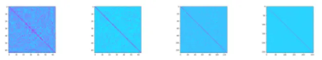
matrix V is supposed to be identity for orthogonal filters. Indeed, considering the SVD decomposition of ℜ(A), V is always orthogonal if the number of filters k is less than maximum rank ofℜ(A) = min(N, whc), with N the number of lines inℜ(A) depending on size of A, strides, and padding. In most situations filters are likely to be naturally orthogonal, except for the first layer of a convolutional network, where the number of input channels is much smaller than those of higher layers, see Figure1. The first convolutional layer in a CNN is the most likely to learn a bank of redundant filters.
Considering smaller or larger strides obviously prevents from reconstructing the input image, see equation2. However, equation4 allows factorization. Smaller strides result in more lines inℜ(A), larger feature maps, and may increase the rank ofℜ(A) for large input channel c.
Fig. 1. Filters covariance matrix of four first convolutional layers of a standard CNN, from left to right (on MNIST dataset).
IV. WEIGHTINGCONVOLUTION
By weighting convolutions, we explicitly consider the (VT
V)−1 term in Eq.5. We further use a diagonal
approxi-mation of this matrix to gain additional degrees of freedom to match a new data distribution when transferring a CNN to a new task.
This process can also help interpreting filters and feature maps contribution, since Σ encodes filter relevancy for the targeted task.
A. Convolution Weighting layer
A convolutional weighting layer scales each of the feature map according to an additional parameter σk so that the kth
feature map Uk is actually computed as follows:
Uk(weig)= σk◦ (ℜ(A) × VkT + bk) (6)
where◦ denotes element-wise scalar to matrix multiplication and bk a bias term.
These k additional parameters σ can be learned by back-propagation. Thus, they are not related to filters variance any-more but act as weights to modulate each filter contribution, according to its relevance to the training objective. This is particularly relevant when adapting pretrained architectures. In this formulation, a standard convolution layer corresponds toΣ = Id.
In practice we insert a Convolution Weighting layer (CWL) after each convolution layer in the CNN that we want to transfer. This layer learns one parameter σk per feature map
k and multiply the whole feature map k by σk according to
B. Transfer Learning with convolution weighting layers This section presents a sketch of a finetuning algorithm that takes advantage of convolutions weights for improved transfer learning. This method is by design more dedicated to limited training size settings.
In algorithm1, we highlight each step when refining a pre-trained model to datasets with possibly very few labels. Steps 1, 2 and 4 correspond to the classical finetuning approach, despite step 1 decreasing the learning rate for convolution layers rather than freezing them. In step 3, we insert a Convolution Weighting Layer after each convolutional layer, or batch normalization if any. This layer learns a vector of dimension k corresponding to the number of feature maps output from its previous convolutional layer. In the forward pass, a feature map Uk is multiplied element-wise by σk as in
equation6. We initialize each σk by1, and let them free for
updating by back-propagation to minimize the network loss during training.
Algorithm 1 Finetuning with weighted convolutions Input: pretrained modelMp, training dataset (X, Y )
Output: finetuned model Mf
1: Mf ← F reezeConvsF ilters(Mp)
2: Mf ← ReplaceClassifLayers(Mf, Y)
3: Mf ← InsertW eightConvs(Mf)
4: Mf ← T rainUnfreezedLayers(Mf, X, Y)
5: return Mf
C. Pruning with convolution weighting layers
When transferring a pretrained architecture to another dataset, some parameters can become unnecessary. For in-stance, transferring to a new task where data exhibits less vari-ability will generally require smaller architectures. Network pruning consists in removing the less important parameters of a network. This section shows how we prune a network by weighting convolutions.
In practice we apply a threshold τ on|σk| values learned
during transfer learning and we remove all filters Vk and
feature maps Uk such that|σk| < τ. Removing feature maps
in intermediate convolution layers reduces the amount of input channels in the following convolutions layers. This drastically reduces the computing complexity of pruned networks while preserving enough information, since fewer filters are needed to approximate the reconstruction of less complex and lower dimensional inputs by UΣV factorization.
This pruning method can be then linked to low-rank com-pression approaches, as learning less filters corresponds to a lower Kronecker rank (equation4.
D. Link to channel saliency
Channel Saliency, or Channel Attention, is the mechanism able to focus the attention within channels of convolutional layers. Several works already study this direction for various goals. Some works [40] are interested in enhancing CNN performance and interpretability by adding attention to both
spatial and channel domains. Alternative works add spatial pooling and/or a parallel MLP to learn non-linear interaction between channels [41]. A similar mechanism is used in [14] to obtain compressed networks at inference time. Such strategies show positive impact, often at the cost of more parameters in a fully supervised learning setting. To the best of our knowledge, channel saliency has not been used for both transfer learning and pruning networks.
V. EXPERIMENTS
We conducted experiments on two main settings: transfer learning for classification, and transfer for image retrieval. We also illustrate few results in network pruning and give an explanation of channel pruning in CNN through the Kronecker factorization analysis presented in sectionIII.
A. Transfer for classification
We explore the capabilities of weighting convolutions to transfer knowledge from the Imagenet dataset to another dataset with few training samples. Three datasets are consid-ered: MIT 67 Scenes, Kvasir v2, and Chest X-ray, and we randomly select few training images per class for each of them. Two architectures are compared, namely VGG-16 and ResNet50. We further evaluate four strategies: as baselines, Finetune and Freeze correspond to standard transfer ap-proaches, whether convolutional layers are trainable of not. We compare these two methods with the proposed Weighting Convolution Layers, see TableIandII.
1) Datasets: We study three image classification datasets from various fields in order to study the impact of dataset shift in transfer learning.
a) MIT 67 Scenes [27]: is an indoor scenes dataset composed of 6,700 images divided in 5,360 training images (around 80 per class) and 1,340 test images (around 20 per class).
b) Kvasir v2 [26]: is a medical image classification dataset aiming at recognizing anatomical landmarks, patho-logical findings, or endoscopic procedures inside the gastroin-testinal tract. The dataset contains 8,000 images with 1,000 image per category. For each class, we divided the dataset into 750 images for training and 250 for testing. Categories include Z-line, pylorus, cecum, esophagitis, polyps, ulcerative colitis, dyed and lifted polyps and dyed resection margins.
c) Chest X-ray [15]: is a second medical image classi-fication dataset aiming at recognizing pneumonia for patients aged between one and five years old. The data is composed of 5,216 training images and 624 test images and has 2 categories whether the patient is normal or infected by pneumonia.
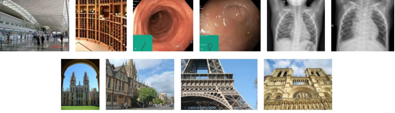
These datasets are selected as they increasingly differ from the original data on which the network is originally trained, while having comparable resolution. MIT 67 has images taken with similar digital cameras as ImageNet, but shows scenes as opposed to objects. Thus, the information to capture is more global than localized objects from ImageNet. Kvasir has digital colored images of the intestine, which has specific shape,
Fig. 2. Images of the datasets used in the experiments: MIT 67 indoor scenes, Kvasir intestine images, chest X-ray for pneumonia recognition, Oxford and Paris landmarks.
color, and organization. Finally, the chest dataset is composed of uncolored images with similar view of patient chest.
We believe that medical images are a great example where transfer require the most adaptation. The first line in figure
2 shows two image samples from each of the three datasets described above.
2) Experimental details: The experiments are performed by using all convolutional layers from a pretrained network and adding a final fully connected layer with as many neurons as categories.
We restrict the training set of the presented datasets by randomly selecting 1, 3, 5, and 10 examples per class to refine the pretrained convolutional model and transfer to the new dataset.
The learning rate is grid searched with values in [0.00001, 0.00005, 0.0001, 0.0005, 0.001] for finetuning runs and in [0.001, 0.005, 0.01, 0.05] for the freeze experiments. Tables below show averages and standard deviations of the best accuracies (over LR), repeated 10 times.
3) Results: First, we study how transfer with Weighting Convolution Layers compares with the standard freeze strat-egy, on the three datasets with the two models, see Table I. We observe that weighting convolution significantly improves over frozen convolutions for most cases. Furthermore, VGG-16 shows more improvements than ResNet, which can be explained by the fact that VGG-16 does not include batch normalization, nor residual connections that helps the model to generalize. We note that the variance is quite high, e.g. more than 10%, for a few experiments with 1 or 3 samples to learn from, which is expected since samples are randomly picked.
Secondly, we study Weighting Convolutions Layers added while finetuning VGG-16 with the same datasets see TableII. We show again that convolutions weights offer improvements even in the case of finetuning on small amount of examples. Also, finetuning outperforms frozen convolutions for Kvasir and Chest datasets, but does not on MIT-67. This can be explained by the fact that these medical datasets require more adaptation than MIT.
B. Transfer for Image Retrieval
To further investigate the transfer capabilities of our method, we study the image retrieval problem. Image retrieval (or content-based image retrieval) aims at searching images in a database that are similar to a given query. In fact, the entire image database is sorted in terms of similarity to given queries. Commonly, pretrained networks are finetuned on large un-supervised or weakly un-supervised datasets that are related to the studied datasets [28], [9]. For instance, network are fine-tuned on a dataset of building images to further perform retrieval on landmarks datasets. Such finetuning is often based on pair or triplet losses, as datasets are not fully annotated.
In our case, we are not interested in finetuning networks on large quantities of weakly annotated data. We rather propose to explore the potential of our method by transferring to the given query images, see TableIII. Therefore, we apply finetuning on the 70 query images of the datasets corresponding to the 15 landmarks. These labels are used to finetune the network as in the classification setting.
1) Datasets: The most common retrieval datasets are Ox-ford5k [24] and Paris6k [25]. Recently, [29] proposed a revisited version of the datasets, ROxford5k and RParis6k, with 15 extra query images corresponding to 5 new landmarks and three evaluation protocols: Easy, Medium, and Hard.
a) ROxford5k: contains 4,993 images with 70 query images corresponding to 16 oxford landmarks.
b) RParis6k: contains 6,322 images with similarly 70 queries of 16 parisian buildings.
The second line in figure2shows two images from the two datasets considered in this section.
2) Experimental details: To evaluate the performance of our method, we compute the common MAC (Maximum Ac-tivations of Convolutions) representation [37] on the VGG-16 and ResNet50 networks. MAC performs global max-pooling on the final convolutional layer of a given network. This vector has a dimension equal to the number of filters on the last con-volutional layer. To perform the evaluation, descriptors are l2-normalized and cosine similarity is computed to rank similarity between queries and images of the dataset. The mean Average Precision (mAP) is finally computed as evaluation metric. We
training data / class 1 3 5 10 VGG-16 MIT 67 Scenes Freeze 0.065 (0.013) 0.178 (0.017) 0.243 (0.013) 0.381 (0.022) Freeze + CWL 0.118(0.010) 0.236(0.021) 0.301(0.024) 0.411(0.014) Kvasir v2 Freeze 0.262 (0.047) 0.399 (0.044) 0.531 (0.030) 0.623 (0.026) Freeze + CWL 0.294(0.050) 0.500(0.041) 0.550(0.017) 0.677(0.023) Chest X-ray Freeze 0.590(0.072) 0.650 (0.121) 0.731 (0.030) 0.795 (0.071) Freeze + CWL 0.587 (0.116) 0.688(0.067) 0.756(0.020) 0.810(0.041) ResNet50 MIT 67 Scenes Freeze 0.166 (0.010) 0.316(0.010) 0.400 (0.010) 0.510(0.016) Freeze + CWL 0.170(0.011) 0.314 (0.021) 0.405(0.014) 0.501 (0.023) Kvasir v2 Freeze 0.345 (0.032) 0.564 (0.039) 0.653 (0.026) 0.752 (0.033) Freeze + CWL 0.356(0.055) 0.568(0.065) 0.664(0.036) 0.759(0.025) Chest X-ray Freeze 0.712 (0.054) 0.696(0.129) 0.757 (0.065) 0.821 (0.028) Freeze + CWL 0.714(0.048) 0.689 (0.127) 0.774(0.049) 0.826(0.030) TABLE I
CLASSIFICATION ACCURACY ONMIT 67, KVASIR,ANDCHEST FORVGG-16ANDRESNET50WITH FROZEN CONVOLUTION AND WEIGHTING CONVOLUTIONS.
training data / class 1 3 5 10
VGG-16 MIT 67 Scenes Finetune 0.058(0.005) 0.108 (0.011) 0.143 (0.008) 0.259(0.014) Finetune + CWL 0.058(0.007) 0.118(0.022) 0.158(0.015) 0.251 (0.020) Freeze 0.065 (0.013) 0.178 (0.017) 0.243 (0.013) 0.381 (0.022) Kvasir v2 Finetune 0.288 (0.082) 0.464 (0.145) 0.533 (0.001) 0.698(0.016) Finetune + CWL 0.309(0.132) 0.536(0.022) 0.590(0.023) 0.666 (0.001) Freeze 0.262 (0.047) 0.399 (0.044) 0.531 (0.030) 0.623 (0.026) Chest X-ray Finetune 0.542 (0.118) 0.684 (0.132) 0.672 (0.163) 0.811 (0.027) Finetune + CWL 0.610(0.086) 0.730(0.138) 0.691(0.114) 0.824(0.031) Freeze 0.590 (0.072) 0.650 (0.121) 0.731 (0.003) 0.795 (0.071) TABLE II
CLASSIFICATION ACCURACY ONMIT 67, KVASIR,ANDCHEST FORVGG-16WITH FINETUNING AND WEIGHTING CONVOLUTIONS.
note that in the case of weighted convolution or finetuning, the last fully connected layer is removed to compute the MAC.
The performance of the four strategies are evaluated, Freez-ing convolutions beFreez-ing the baseline as the MAC from [37]. We note that MAC is computed given images with original size as input to the network. The training is performed by giving images with a fixed size of 1024 × 768. Furthermore, data augmentation is performed to cope with the various image orientations, when learning. Finally, the learning rate is grid searched as for image classification.
3) Results: As for classification, the performance of the four strategies is evaluated, see TableIII. VGG-16 and ResNet are evaluated on ROxford and RParis in the Easy, Medium, and Hard settings. The average performance is also given.
We observe that weighting convolutions brings improve-ments over both freezing and finetuning strategies in all cases. Thus, adapting representations by transferring models using weighting convolutions is also beneficial in the image retrieval setting. Furthermore, finetuning offers better performance than freezing, which is explained by the fact that the network is
originally designed to take224 × 224 dimensional images as input and finetuning allows it to adapt to a larger resolution, as in the evaluation.
C. Pruning
We further study network pruning based on the convolution weights. Different compression levels are evaluated and the classification accuracy of the pruned models are shown before and after finetuning. Specifically, Table IVshows the perfor-mance of a pruned VGG-16 model, transferred from ImageNet to Kvasir with 50 samples per class, as well as the compression ratio of both the model parameters and the feature maps. We observe that the number of parameters, respectively feature maps can be reduced to 45%, respectively 74%, at the cost of 1.5% accuracy. Furthermore, massive compression of 1% of the parameters and 16% or the feature maps reduce the accuracy to65.8% from 90.4% with the original model.
This pruning method can be related to low-rank compression approaches as mentioned above. Since filters removal leads to activations removal, this cascading effect significantly damage
ROxford5k RParis6k
Easy Medium Hard Mean Easy Medium Hard Mean VGG-16 Original / Freeze 49.37 37.09 15.21 33.89 60.88 47.79 25.16 44.61 Freeze + CWL 50.70 37.80 14.55 34.35 62.42 48.85 24.33 45.20 Finetune 41.07 33.23 12.78 29.03 65.63 51.58 27.08 48.10 Finetune + CWL 49.53 39.08 15.30 34.64 69.21 53.26 27.08 49.85 ResNet50 Original / Freeze 41.98 32.99 13.87 29.61 62.51 46.44 21.88 43.61 Freeze + CWL 55.27 42.35 16.08 37.90 77.43 56.09 27.18 53.57 Finetune 62.95 51.30 25.02 46.42 82.33 64.79 38.93 62.02 Finetune + CWL 63.19 51.21 25.31 46.57 82.95 66.16 42.52 63.88 TABLE III
RETRIEVAL PERFORMANCE ONROXFORD5K ANDRPARIS6K FORVGG-16ANDRESNET.
the network capability without the finetuning phase. We ob-serve in table IV that only one epoch of finetuning already boost accuracy for the highest compression rates.
τ Acc. FT@1 FT@30 #Param #Feat
- 0.904 - - 100% 100% 0.2 0.905 0.890 0.909 95% 98% 0.4 0.892 0.888 0.907 85% 96% 0.8 0.492 0.858 0.889 48% 74% 1.0 0.221 0.635 0.825 23% 44% 1.2 0.121 0.533 0.658 1% 16% TABLE IV
PRUNING ONKVASIR WITHVGG-16
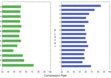
Figure3shows compression rate for every convolution layer of VGG-16 and ResNet50 architectures, after transferring from ImageNet to Kvasir dataset, using τ = 0.8 and 50 samples per class. We observe more pruned filters in lower layers for VGG architecture transferred to Kvasir dataset. This is due to the high redundancy of the first layer as discussed in section
III-C. For the ResNet50 architecture, the figure shows every convolution layers corresponding to 3 × 3 filters. We observe similar high compression rate in the lowest layer, as well as in the highest layers. Since highest layers in CNNs are known to learn high-level features related to the dataset categories, the high pruning ratio in higher layers confirm that only the most relevant filters are transferred and pruned to handle the targeted dataset.
VI. CONCLUSION
This paper proposes a simple yet efficient transfer learning method for convolutional neural network. Our approach is grounded by a formal analysis of the convolution operation, providing evidence of a tight connection with Kronecker factorization. Additional vectors for weighting convolution feature maps are introduced, allowing more degrees of free-dom to the network for transfer learning with few samples. Our approach is validated with two CNN architectures on five datasets of image classification or retrieval. Based on the con-volutions weights, we further experiment network pruning to compress transferred models. Interestingly, high compression rates can be obtained for both parameters and activations, i.e. feature maps, while preserving good performance. Finally, our
Fig. 3. Compression rate per layer using VGG-16 (left) and ResNet50 (right) architectures on Kvasir dataset
formalization allows a better understanding of convolutional channel pruning when transferring pretrained models.
ACKNOWLEDGMENTS
This work was funded in part by the French Agence Na-tionale de la Recherche (grants number ANR16-CE23-0006 and ANR-19-CE23-0009-01). Centre de Calcul Intensif d’Aix-Marseille is acknowledged for granting access to its high performance computing resources.
REFERENCES
[1] Liang-Chieh Chen, George Papandreou, Iasonas Kokkinos, Kevin Mur-phy, and Alan L Yuille. Deeplab: Semantic image segmentation with deep convolutional nets, atrous convolution, and fully connected crfs.
IEEE transactions on pattern analysis and machine intelligence, 40:834– 848, 2017. 2
[2] Wenlin Chen, James Wilson, Stephen Tyree, Kilian Weinberger, and Yixin Chen. Compressing neural networks with the hashing trick. In
Proceedings of the 32nd International Conference on Machine Learning, 2015. 2
[3] Yu Cheng, Duo Wang, Pan Zhou, and Tao Zhang. A survey of model compression and acceleration for deep neural networks, 2017. 2 [4] Saheb Chhabra, Puspita Majumdar, Mayank Vatsa, and Richa Singh.
Data fine-tuning. In Conference on Artificial Intelligence (AAAI), 2019. 2
[5] Vincent Dumoulin and Francesco Visin. A guide to convolution arithmetic for deep learning, 2016. 3
[6] Dumitru Erhan, Yoshua Bengio, Aaron Courville, Pierre-Antoine Man-zagol, Pascal Vincent, and Samy Bengio. Why does unsupervised pre-training help deep learning? Journal of Machine Learning Research, 11:625–660, 2010.1
[7] Yaroslav Ganin, Evgeniya Ustinova, Hana Ajakan, Pascal Germain, Hugo Larochelle, Franc¸ois Laviolette, Mario Marchand, and Victor Lempitsky. Domain-adversarial training of neural networks. Journal
of Machine Learning Research (JMLR), 17:2096–2030, 2016. 2 [8] Timur Garipov, Dmitry Podoprikhin, Alexander Novikov, and Dmitry P.
Vetrov. Ultimate tensorization: compressing convolutional and fc layers alike. ArXiv, 2016.1
[9] Albert Gordo, Jon Almazan, Jerome Revaud, and Diane Larlus. End-to-end learning of deep visual representations for image retrieval. arXiv
preprint arXiv:1610.07940, 2016. 5
[10] Yunhui Guo, Honghui Shi, Abhishek Kumar, Kristen Grauman, Tajana Rosing, and Rogerio Feris. Spottune: Transfer learning through adaptive fine-tuning. In The IEEE Conference on Computer Vision and Pattern
Recognition (CVPR), 2019.2
[11] Song Han, Jeff Pool, John Tran, and William Dally. Learning both weights and connections for efficient neural network. In Advances in
Neural Information Processing Systems (NIPS), pages 1135–1143. 2015. 2
[12] Kaiming He, Georgia Gkioxari, Piotr Doll´ar, and Ross Girshick. Mask r-cnn. In Proceedings of the IEEE international conference on computer
vision, pages 2961–2969, 2017.2
[13] Yihui He, Xiangyu Zhang, and Jian Sun. Channel pruning for accelerat-ing very deep neural networks. In Proceedaccelerat-ings of the IEEE International
Conference on Computer Vision, pages 1389–1397, 2017. 1
[14] Jie Hu, Li Shen, Gang Sun, and Samuel Albanie. Squeeze-and-excitation networks. IEEE Transactions on Pattern Analysis and Machine
Intelli-gence, 2017. 4
[15] Daniel Kermany, Kang Zhang, and Michael Goldbaum. Labeled optical coherence tomography (oct) and chest x-ray images for classification.
Mendeley data, 2, 2018. 4
[16] Vadim Lebedev, Yaroslav Ganin, Maskim Rakhuba, and Ivan V. Os-eledets. Speeding-up convolutional neural networks using fine-tuned cp-decomposition. CoRR, 2014.1,2
[17] Yann LeCun, John S Denker, and Sara A Solla. Optimal brain damage. In Advances in neural information processing systems, pages 598–605, 1990.2
[18] Mingsheng Long, Yue Cao, Jianmin Wang, and Michael I. Jordan. Learning transferable features with deep adaptation networks. In
Proceedings of the 32nd International Conference on International Conference on Machine Learning (ICML), page 97–105. JMLR.org, 2015.2
[19] Pavlo Molchanov, Stephen Tyree, Tero Karras, Timo Aila, and Jan Kautz. Pruning convolutional neural networks for resource efficient transfer learning. 2017. 1,2
[20] K. Nan, S. Liu, J. Du, and H. Liu. Deep model compression for mobile platforms: A survey. Tsinghua Science and Technology, 24, 2019. 2 [21] Alexander Novikov, Dmitry Podoprikhin, Anton Osokin, and Dmitry P.
Vetrov. Tensorizing neural networks. In NIPS, 2015. 1,2
[22] Sinno Jialin Pan, Ivor W Tsang, James T Kwok, and Qiang Yang. Domain adaptation via transfer component analysis. IEEE Transactions
on Neural Networks, 22(2):199–210, 2010. 1
[23] Bo Peng, Wenming Tan, Zheyang Li, Shun Zhang, Di Xie, and Shiliang Pu. Extreme network compression via filter group approximation. In
Proceedings of the European Conference on Computer Vision (ECCV), pages 300–316, 2018. 1
[24] James Philbin, Ondrej Chum, Michael Isard, Josef Sivic, and Andrew Zisserman. Object retrieval with large vocabularies and fast spatial matching. In 2007 IEEE conference on computer vision and pattern
recognition, pages 1–8, 2007.5
[25] James Philbin, Ondrej Chum, Michael Isard, Josef Sivic, and Andrew Zisserman. Lost in quantization: Improving particular object retrieval in large scale image databases. In 2008 IEEE conference on computer
vision and pattern recognition, pages 1–8, 2008. 5
[26] Konstantin Pogorelov, Kristin Ranheim Randel, Carsten Griwodz, Sigrun Losada Eskeland, Thomas de Lange, Dag Johansen, Con-cetto Spampinato, Duc-Tien Dang-Nguyen, Mathias Lux, Peter Thelin Schmidt, Michael Riegler, and P˚al Halvorsen. Kvasir: A multi-class image dataset for computer aided gastrointestinal disease detection. In Proceedings of the 8th ACM on Multimedia Systems Conference, MMSys’17, pages 164–169, 2017.4
[27] Ariadna Quattoni and Antonio Torralba. Recognizing indoor scenes. In
2009 IEEE Conference on Computer Vision and Pattern Recognition,
pages 413–420, 2009. 4
[28] Filip Radenovi´c, Giorgos Tolias, and Ondˇrej Chum. Cnn image retrieval learns from bow: Unsupervised fine-tuning with hard examples. In
European conference on computer vision, pages 3–20, 2016.5 [29] Filip Radenovi´c, Ahmet Iscen, Giorgos Tolias, Yannis Avrithis, and
Ondˇrej Chum. Revisiting oxford and paris: Large-scale image retrieval benchmarking. In The IEEE Conference on Computer Vision and Pattern
Recognition (CVPR), 2018. 5
[30] Joseph Redmon, Santosh Divvala, Ross Girshick, and Ali Farhadi. You only look once: Unified, real-time object detection. In Proceedings of
the IEEE conference on computer vision and pattern recognition, pages 779–788, 2016. 2
[31] Shaoqing Ren, Kaiming He, Ross Girshick, and Jian Sun. Faster r-cnn: Towards real-time object detection with region proposal networks. In
Advances in neural information processing systems, pages 91–99, 2015. 2
[32] Hongje Seong, Junhyuk Hyun, and Euntai Kim. Fosnet: An end-to-end trainable deep neural network for scene recognition. arXiv preprint
arXiv:1907.07570, 2019. 2
[33] Pierre Stock, Armand Joulin, R´emi Gribonval, Benjamin Graham, and Herv´e J´egou. And the bit goes down: Revisiting the quantization of neural networks. In ICLR, 2020. 2
[34] Baochen Sun, Jiashi Feng, and Kate Saenko. Correlation Alignment for
Unsupervised Domain Adaptation, pages 153–171. 2017.2
[35] Qianru Sun, Yaoyao Liu, Tat-Seng Chua, and Bernt Schiele. Meta-transfer learning for few-shot learning. In The IEEE Conference on
Computer Vision and Pattern Recognition (CVPR), 2019. 1
[36] Nima Tajbakhsh, Jae Y Shin, Suryakanth R Gurudu, R Todd Hurst, Christopher B Kendall, Michael B Gotway, and Jianming Liang. Con-volutional neural networks for medical image analysis: Full training or fine tuning? IEEE transactions on medical imaging, 35:1299–1312, 2016. 1
[37] Giorgos Tolias, Ronan Sicre, and Herv´e J´egou. Particular object retrieval with integral max-pooling of CNN activations. 2016. 5,6
[38] E. Tzeng, J. Hoffman, K. Saenko, and T. Darrell. Adversarial discrimi-native domain adaptation. In 2017 IEEE Conference on Computer Vision
and Pattern Recognition (CVPR), 2017. 2
[39] Charles F Van Loan and Nikos Pitsianis. Approximation with kronecker products. In Linear algebra for large scale and real-time applications, pages 293–314. Springer, 1993. 2
[40] Fei Wang, Mengqing Jiang, Chen Qian, Shuo Yang, Cheng Li, Honggang Zhang, Xiaogang Wang, and Xiaoou Tang. Residual attention network for image classification. pages 6450–6458, 2017. 4
[41] Sanghyun Woo, Jongchan Park, Joon-Young Lee, and In-So Kweon. Cbam: Convolutional block attention module. In ECCV, 2018. 4 [42] Jun Yang, Rong Yan, and Alexander G Hauptmann. Adapting svm
clas-sifiers to data with shifted distributions. In Seventh IEEE International
Conference on Data Mining Workshops (ICDMW 2007), pages 69–76, 2007. 1
[43] Wei Ying, Yu Zhang, Junzhou Huang, and Qiang Yang. Transfer learning via learning to transfer. In International Conference on Machine
Learning, pages 5072–5081, 2018.1
[44] Jason Yosinski, Jeff Clune, Yoshua Bengio, and Hod Lipson. How transferable are features in deep neural networks? In Proceedings of
the 27th International Conference on Neural Information Processing Systems (NIPS), pages 3320–3328, 2014. 1
[45] Xiyu Yu, Tongliang Liu, Xinchao Wang, and Dacheng Tao. On compressing deep models by low rank and sparse decomposition. In The
IEEE Conference on Computer Vision and Pattern Recognition (CVPR), 2017. 2
[46] Amir R Zamir, Alexander Sax, William Shen, Leonidas J Guibas, Jitendra Malik, and Silvio Savarese. Taskonomy: Disentangling task transfer learning. In Proceedings of the IEEE Conference on Computer
Vision and Pattern Recognition, pages 3712–3722, 2018. 1 [47] Lei Zhang. Transfer adaptation learning: A decade survey, 2019. 1 [48] Chenglong Zhao, Bingbing Ni, Jian Zhang, Qiwei Zhao, Wenjun Zhang,
and Qi Tian. Variational convolutional neural network pruning. In The
IEEE Conference on Computer Vision and Pattern Recognition (CVPR), 2019. 1,2
[49] Z. Zhou, J. Shin, L. Zhang, S. Gurudu, M. Gotway, and J. Liang. Fine-tuning convolutional neural networks for biomedical image analysis: Actively and incrementally. In CVPR, pages 4761–4772, 2017. 1