HAL Id: hal-01704516
https://hal.archives-ouvertes.fr/hal-01704516
Submitted on 30 Apr 2021
HAL is a multi-disciplinary open access
archive for the deposit and dissemination of
sci-entific research documents, whether they are
pub-lished or not. The documents may come from
teaching and research institutions in France or
abroad, or from public or private research centers.
L’archive ouverte pluridisciplinaire HAL, est
destinée au dépôt et à la diffusion de documents
scientifiques de niveau recherche, publiés ou non,
émanant des établissements d’enseignement et de
recherche français ou étrangers, des laboratoires
publics ou privés.
Cluster luminosity function and n
th
ranked magnitude as
a distance indicator
Stéphane Rauzy, C. Adami, A. Mazure
To cite this version:
Stéphane Rauzy, C. Adami, A. Mazure. Cluster luminosity function and n
thranked magnitude as
a distance indicator. Astronomy and Astrophysics - A&A, EDP Sciences, 1998, 337, pp.31.
�hal-01704516�
AND
ASTROPHYSICS
Cluster luminosity function and n
th
ranked magnitude
as a distance indicator
⋆,⋆⋆
S. Rauzy1, C. Adami2, and A. Mazure2
1
Centre de Physique Theorique, Marseille, France
2
IGRAP, Laboratoire d’Astronomie Spatiale, Marseille, France Received 20 April 1998 / Accepted 4 June 1998
Abstract. We define here a standard candle to determine the
distance of clusters of galaxies and to investigate their pecu-liar velocities by using the nth rank galaxy (magnitude mn).
We address the question of the universality of the luminosity function for a sample of 28 rich clusters of galaxies (cz≃20000 km.s−1) in order to model the influence on m
nof cluster
rich-ness. This luminosity function is found to be universal and the fit of a Schechter profile gives α=-1.50±0.11 and Mbj∗=-19.91
±0.21 in the range [-21,-17]. The uncorrected distance indica-tor mnis more efficient for the first ranks n. With n=5, we have
a dispersion of 0.61 magnitude for the (mn,5log(cz)) relation.
When we correct for the richness effect and subtract the back-ground galaxies we reduce the uncertainty to 0.21 magnitude with n=15. Simulations show that a large part of this dispersion originates from the intrinsic scatter of the standard candle it-self. These provide upper bounds on the amplitude σvof cluster
radial peculiar motions. At a confidence level of 90%, the
dis-persion is 0.13 magnitude and σvis limited to 1200 km.s−1for
our sample of clusters.
Key words: cosmology: distance scale – cosmology:
large-scale structure of Universe – galaxies: clusters – galaxies: lumi-nosity function
1. Introduction
Distances of clusters of galaxies are obtained by measuring the redshift of the galaxies inside the clusters. However, some local mass concentrations could induce peculiar motions superim-posed to the Hubble flow (e.g. Bahcall & Oh 1996). Measure-ments of these peculiar motions which have important conse-quences on cosmological models, require the use of independent distance estimates.
One of the methods uses the Fundamental Plane (FP here-after) of clusters of galaxies (e.g. Schaeffer et al. 1993, for 16 clusters with a median redshift of 0.04). Adami et al. (1998:
Send offprint requests to: C. Adami
⋆
Based on observations collected at the European Southern Obser-vatory (La Silla, Chile)
⋆⋆
http://www.astrsp-mrs.fr/www/enacs.html
A98a hereafter, for 29 clusters with a median redshift of 0.07) show in this way a limit for the peculiar cluster motions of less than 1000 km.s−1. However, the use of the FP as a distance
indicator is not easy: the determination of the total luminosity requires highly accurate photometry and the determination of the core radius requires the positions of the members galax-ies. Finally, to have a reliable velocity dispersion, more than 10 redshifts (interlopers removed) are needed. It is also common to use the tenth rank galaxy as a standard candle (e.g. Abell, Corwin & Olowin 1989: ACO hereafter) to find the distance. Bahcall & Oh (1996) use a sample of cluster velocities based on Tully Fisher distances of Sc galaxies for the same goal. Colless (1995), Hudson & Ebeling (1997) or Lauer & Postman (1994) use also the slope of the brightness profile of the cD galaxies to deduce the distance. Using these different methods, these au-thors constrain the peculiar velocities of different samples of nearby clusters (z≤0.05).
To re-address these questions, we develop in this work a new distance indicator using the galaxy of the nthrank for a given cluster. We use the ENACS (see Katgert et al. 1996, Mazure et al. 1996, Biviano et al. 1997, A98a, Katgert et al. 1998 (K98), Adami et al. 1998 (A98b) and de Theije et al. 1998) and COS-MOS (e.g. Heydon Dumbleton et al. 1989) data. To estimate correctly this indicator, we look at the possible universality of the Luminosity Function for clusters of galaxies (LF hereafter), after taking into account the correction for parameters such as the number of galaxies in the cluster. The universality of the LF is for example treated in Lumsden et al. (1997: L97 hereafter), in Valotto et al. (1997: V97 hereafter) or in Trentham (1998). L97 and V97 derive synthetic LF’s for samples of clusters of galax-ies. V97 found a significant difference between the rich and the poor clusters, while L97 found a significant difference between the high and low velocity dispersion clusters. These two studies use the COSMOS/EDSGC data. For V97, the redshifts of the clusters come from a literature compilation.
In order to study these points and to investigate the exis-tence of a standard candle, we will proceed as follow: In the first section we describe the selected sample. We determine in the second section the luminosity function and we look for its universality, at least in the magnitude range [-21;-17]. In the third section, we redefine mn as a distance indicator and
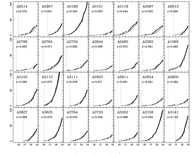
cor-32 S. Rauzy et al.: Cluster luminosity function and nthranked magnitude as a distance indicator,
Fig. 1a and b. Illustration of the reconstruction method (see text in Sect. 3.1. for explanations) of the individual and composite luminosity
functions.
rect it for the influence of background level, the richness of the clusters and the statistical effects and we use it to examine the peculiar motions of the ENACS/COSMOS clusters of galaxies.
We use in this article H0=100 km.s−1.Mpc−1and q0=0.
2. The sample
In this work, we use the ENACS and COSMOS surveys. They are well described in K98. ENACS gives the redshifts and the R25calibrated magnitude and COSMOS the positions and the bj
magnitudes for all galaxies in the clusters. K98 show that clus-ters for which the photometry in the two catalogues is based on the same survey plate, the two magnitude scales agree very well. There do not appear to be serious problems with either magnitude scale. In addition, some redshifts come from the lit-erature. The absolute magnitudes have been computed by using the mean cluster redshift and the same K(z)-correction as in L97: K(z)=4.14z-0.44z2. We have also corrected for galactic extinc-tion using the map of Burstein & Heiles (1982) in the same way as in A98a. The redshifts are calculated with respect to the rest frame of the Cosmic Microwave radiation (CMR hereafter) defined by Lubin & Villela (1986).To reduce the substructure effects and to have good measurements of the different cluster parameters such as core radius, velocity dispersion, mean
red-shift, background level and number of galaxies on the line of sight, we limit the global sample to the 29 most regular clus-ters in A98a. These clusclus-ters have an Abell richness greater than 1. They do not have major 2D visible substructure. We take only the unatypical King core radii (we have removed A3128 which exhibits a large core radius). For these final 28 clusters we consider galaxies within 5 King core radii (about 500 kpc). According to K98, we know that COSMOS has a complete-ness level of 91% for bj≤19.5. However, this estimate refers to
areas with high surface density in the COSMOS catalogue. For low surface density of galaxies (outside the clusters), the com-pleteness level in certainly higher. To increase the comcom-pleteness, we add to the COSMOS objects, the ENACS ones not found in the given area and inside the clusters. Finally, to be sure that we have a complete sample, we limit it to bj≤19. We note also that
we remove the objects with a back- or fore-ground redshift (see Katgert et al. 1996). We have finally more than 3500 galaxies in the global sample. We split the sample into 3 sub-samples to test for spatial variations. The first sub-sample contains the galaxies between 0 and 2 core radii, the second the galaxies between 2 and 3.5 core radii and the third the galaxies between 3.5 and 5 core radii. We have almost 1200 galaxies in each of the three sub-samples.
3. The cluster luminosity function
3.1. The method
In order to test the universality of the LF for our 28 clusters, we construct from the present data this function. We use a method similar to those used for example in Beers& Tonry (1986) or
Merrifield & Kent (1989) for the density profiles reconstruction. We take into account the different limiting magnitudes of the different clusters. We consider the composite cumulative LF (CCLF hereafter, noted F(M) in the figures). L97 use a similar (Colless 1989) reconstruction method, while V97 simply add the individual clusters with a common limiting apparent magnitude of 19.4.
First of all, we remove statistically the background objects in each cluster. The mean number of removed objects is the mean number of background objects minus the number of al-ready removed objects on the basis of the redshift. The mean number of background objects comes from a density profile fit, including as a free parameter the background density (A98a and b ). A98a and b have shown that this background estimation is very robust and in good agreement with the count law of field galaxies. It represents about 44% of the total number of
galax-ies along the line of sight. Starting from a limiting magnitude of
bj=20, we have rescaled this number for bj=19 (for better
com-pleteness) by using the count law of L97 in order to calculate the proportion of galaxies in each magnitude bin. We also use this law to select the magnitude of the background removed objects. To obtain a statistical error, we have made 100 calculations of the cumulative LF for each cluster (CLF hereafter), taking into account the internal background fluctuation (i.e. the error in the determination of the mean number of background objects for each cluster).
As described above, we have applied to construct the CCLF an adapted version of the method devised for example by Beers and Tonry (1986) for the cluster density profiles.
We denote by Mlimk = mclim−µ(z) the corrected absolute
magnitude limit of the kthfarthest clusters. Up to each Mlimk we compute the cumulative count Gk(M ) of all the galaxies
belonging to the set of clusters i complete in M i.e. verify-ing Mlimi ≤Mlimk (hereafter these galaxies samples are called
Sk). While these cumulative counts Gk(M ) are not affected
by incompleteness problems, they suffer from sampling errors as k increases (i.e. because the number of selected clusters de-creases with distance, the number of galaxies in sample Skfor
a given absolute magnitude range is a decreasing function of
k). Fig. 1(a) illustrates this behaviour: the Gk(M ) of samples
Sk are plotted. The cut-off Mlimk are indicated as dotted lines.
The number of clusters contributing to a Gk(M ) decreases with
Mk
lim. In order to minimize sampling errors, we adopt the
fol-lowing rescaling procedure for reconstructing the CCLF. For an increasing cut-off Mlimk , rescaled cumulative counts Fk+1(M )
are defined recursively as follows
Fk+1(M ) =
Gk+1(Mlimk )
Fk(Mlimk )
Fk(M ) if M ≤ Mlimk
Fk+1(M ) = Gk+1(M ) if Mlimk < M ≤ Mlimk+1
Fig. 2. Final CCLF with errors. The filled surface represents the
enve-lope (the error) of the CCLF due to the field subtraction and the dotted envelope takes into account the statistical fluctuations. The CCLF is normalized to 1 for M=-19.5.
with F1(M ) = G1(M ). It consists in replacing up to Mlimk
the cumulative counts Gk+1(M ) by the reconstructed CCLF
Fk(M ) renormalized such that continuity of the final CCLF
is ensured. The sampling errors are thus minimized (Fk(M )
are plotted Fig. 1(b) for comparison) since Fk(M ) is estimated
using information provided by all the sampled clusters while cumulative count estimate Gk+1(M ) use only the set of ith
clusters verifying Mlimi ≤Mlimk+1. Such a procedure warrants an optimal reconstruction of the cumulative luminosity function of galaxies belonging to a sample of clusters spread in redshifts. The final CCLF is shown in Fig.2, arbitrarily normalized at 1 for M=-19.5. It spans a range of 4 absolute magnitudes M be-tween -21 and -17. The lower limit allows us to exclude the very bright galaxies (cD galaxies) which are probably not belonging to the mean luminosity function. The upper limit corresponds to the absolute magnitude of the faintest galaxy with mlim=19 in
the nearest cluster. L97 have used the range [-21;-18] and V97 the ranges [-21.5;-17] and [-21.5;-16].
This method assumes obviously that the LF’s are similar in the different clusters. We will check afterwards that this condi-tion is well satisfied (see Sect. 3.2.3).
3.2. Analysis
3.2.1. Spatial variations
We looked for spatial variations of the LF. In order to do that, we tested the CCLF in the 3 defined areas. We reconstructed it exactly in the same way as above but for zones enclosed in [0,2] rc (CCLF1), [2,3.5] rc (CCLF2) and [3.5,5]rc (CCLF3).
We superpose the three CCLF’s (Fig. 3) after normalization at 1 for M=-19.5. They look very similar. A Kolmogorov-Smirnov show that CCLF1 and CCLF2 are identical at a confidence level of 95 %. CCLF2 and CCLF3 are identical at a confidence level of only 65%. The conclusion is that the 3 CCLF’s are probably identical (with a high confidence level) and that the LF’s do not vary significantly with the radius. This result is in agreement
34 S. Rauzy et al.: Cluster luminosity function and nthranked magnitude as a distance indicator,
Fig. 3. CCLF’s issued from the three radial bins: [0,2] rc(filled), [2,3.5]
rc(dashed) and [3.5,5] rc(dashed dotted).
with V97, which have used 55 clusters (16 rich clusters). Only 3 of those clusters are common with our sample. They did not find significant variations of the LF within 1 Mpc from the center (roughly 10 core radii).
Moreover, this universality supports our background sub-traction approach. We assumed implicitely that the background is homogeneous inside 5 core radii. The number of removed galaxies in each of the three bins is then directly proportional to the area of these bins. We have thus removed 4 times more galaxies in the exterior bin than in the central one. However, the three reconstructed CCLF’s are very similar, supporting the way we remove the background.
3.2.2. Universality of the LF
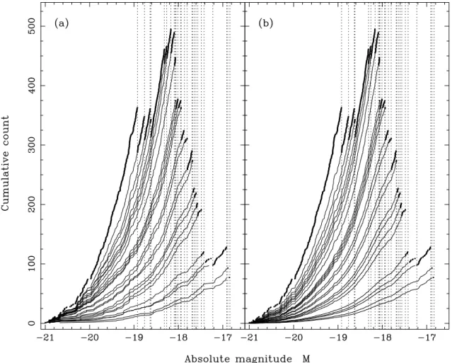
A way to test this point is to compare the individual clusters CLF to the CCLF (Fig. 4). We plot all the individual CLF’s in apparent magnitudes and no subtracted background (G(m) in Fig. 4). We simulate the theoretical no background subtracted CLF’s by adding background objects (L97) to the reconstructed mean CCLF (normalized to the number of galaxies in each clus-ter). We see a good agreement between the observations and the simulations. We can quantify this agreement by using a Kolmogorov-Smirnov test between the observed data and the simulated data. We test the hypothesis that the observations and simulations are drawn from the same parent population. The mean risk is 62% for 80% of the clusters which is a conclusive statement: we have a small dispersion of the individual CLF’s around the mean function, and so the LF is probably universal. If the individual CLF’s are drawn from a universal function, the differences (and so the risks) must be randomly distributed. In order to test this hypothesis, we generate 500 random distri-butions of 28 CLF’s (normalized like each real cluster) around the reconstructed global CCLF.
We proceed with another Kolmogorov Smirnov test and we find a level of 75% to reject the right hypothesis if we assume that the individual risks distribution is non random. As a con-clusion, we can say that the CCLF’s are globally universal for
all our 28 selected rich clusters. This is in agreement with L97 or Trentham (1998). We note that V97 argue against a universal LF, but between the rich and the poor clusters.
3.2.3. Modelisation
Even if the following sections do not use this modelisation, we fit here a Schechter function (1976) to the LF:
S(M ) = Φ∗100.4(α+1)(M∗−M )exp[−100.4(M∗−M )]
whereΦ∗is given by the number of galaxies in each cluster and M∗is the characteristic magnitude. We use the minimization algorithm MINUIT (e.g. A98a). First, we calculate a χ2fit using the weights of the reconstruction. We have α=-1.50 ± 0.11 and Mbj∗=-19.91 ± 0.21. The LF’s calculated with the 3 radial zones
give similar results at the 1 sigma level. If we minimize the maximal distance (divided by weight) between the model and the observations instead of the χ2 (Kolmogorov Smirnov fit: KMS fit hereafter), we have α=-1.47 and Mbj∗=-19.89 (without
reliable errors).
These two results are consistent at the 1 sigma level (ac-cording to the error bars). Morever, we have a difference of less than 2% for α and 1 % for Mbj∗. The parameter determination
is then independent of the fitting method.
These values could also be compared with the recent analy-ses of L97 and V97. They have both used the χ2minimization. V97 have found α=-1.5±0.1 and Mbj∗=-20.0±0.1 for their
rich clusters and for the magnitude range [-21.5;-17]. Those two parameters are in agreement at the 1 sigma level with our KMS or χ2determinations.
L97 find α=-1.22±0.04 and Mbj∗=-20.16±0.02 in the
mag-nitude range [-21,-18]. The result for M∗is also in good agree-ment with our value at the 1 sigma level. However, the α value is only consistent at the 3 sigma level. If we fit into the same magnitude range we find Mbj∗=-20.18±0.20 in perfect
agree-ment with L97, but α=-1.63±0.12 consistent at only 3 sigma. We note that L97 use q0=1, but it has no influence on the M∗
determination.
For individual clusters, we compare with Bernstein et al. (1995) and Lobo et al. (1997). They found respectively α=-1.42±0.05 and α=-1.59±0.02 for the Coma cluster. The two values are consistent with our KMS fit at the 1 sigma level. We note here that these two values are deduced from photometric surveys of the core of the Coma cluster after statistical back-ground subtraction. For the Lobo et al. study, we have considered the result for a Schechter profile fit only.
Nearly all the results cited in the literature are consistent with our parameters. The only discrepancy occurs for the α value of L97. This could be due to two major sources:
-First, Bernstein et al. (1995), L97, V97 or Lobo et al. (1997) remove the background galaxies in a statistical way. The most local corrections are made in L97 and consist in the removal of a uniform background density calculated in an external annulus. But, the radius of this annulus is always greater than 4 Mpc. We show in A98a that the background density may change by a
Fig. 4. The 28 observed CLF’s + background (points). The model CLF’s deduced of the CCLF after normalization + background are superposed
(solid line).
significant factor at these scales. As an example, the two clusters A3825 and A3827 are separated only by about 3 Mpc and the background density for A3825 is 40% higher than for A3827.
Removing the background by using a distant external annulus could then induce a bias.
-Second, L97 use all the COSMOS galaxies brighter than bj=20. We know (see K98) that the COSMOS catalogue in the
area of ENACS clusters is only complete at the 90% level for
bj≤19.5 and we limit here our sample to bj≤19 to be sure to
be complete. The LF’s of L97 could then miss some galaxies in the faint parts, which could lead to a lower α value.
4. The distance indicator
After we have shown that LF’s are universal within the consid-ered magnitude range, we want to test the Hubble flow and to try to determine the peculiar velocities in our sample of clusters of galaxies by using a distance indicator using photometric data.
4.1. Definition of the optimal rank n for the distance determination
Following Jones & Mazure (1993), who have used m′ 15 = 1 11 20 P r=10
mr(where mris the magnitude of the rthranked cluster
galaxy), we search for a similar standard candle. We test here mnwith n∈[1,28]. We first look at the Hubble relation for the
m10magnitude to be coherent with ACO (1989). By using
bi-sector indicators (Isobe et al., 1990), we find a regression slope between m10and log10(cz) of 4.58±1.24 consistent with the
previous ACO results. This is in good agreement with the ex-pected value of 5. So, we will fix hereafter the slope of all the regressions between mnand log10(cz) to a value of 5.
We want now to find the optimal rank to define a distance in-dicator. To deal with the real minimal observing conditions, we use all the projected galaxies: we do not remove from the total sample the fitted number of background galaxies. We compute the basic dispersion of the relations between mnand log10(cz)
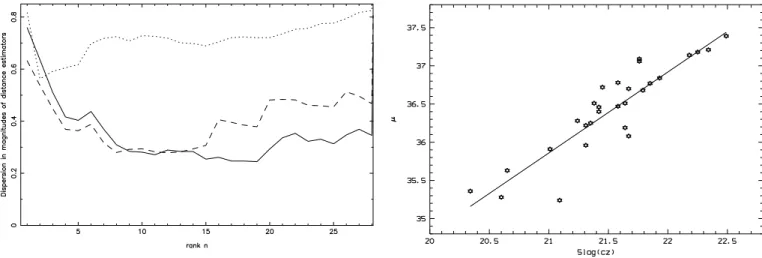
for each n. The best choice is the rank n for which the dispersion is minimal. We see on Fig. 5 that the basic dispersion is mini-mal for the first ranks. If we take for example n=5 (see tab. 1),
36 S. Rauzy et al.: Cluster luminosity function and nthranked magnitude as a distance indicator,
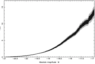
Fig. 5. Dispersions in magnitude according to the rank k. The dotted line
is the first indicator without correction, the dashed line is the indicator corrected for richness and the solid line is the indicator corrected for richness and for background galaxies.
the dispersion is 0.61 magnitude. If we assume as the mean ve-locity of our cluster sample 20000 km.s−1, the corresponding
dispersion in velocity is 5612 km.s−1(0.02 in redshift). We have
m5=5log(cz)-(4.46±0.12).
Clearly, this precision is too low to allow any analysis of the peculiar velocities of the individual clusters.
4.2. Peculiar velocities
The indicator used previously is affected by different intrinsic factors peculiar to each cluster, such as the background level, the richness of the clusters (number of galaxies inside these clusters) and of course the peculiar velocities. We want here to correct for the background and for the richness. To model these two con-tributions, we assume first that in our absolute magnitude range [-21.,-17.], the count law of the background galaxies Gb(m)
is proportional to the canonical exponential: exp(α(m-mlim))
with α the logarithmic slope and mlim the apparent limiting
magnitude (=19.). Second, we note F0(M) (with M the absolute
magnitude) the CLF normalized to unity at M0=-19.5. If µ is
the distance modulus of a given cluster, we have M=m-µ. We deduce then an expression for the rank k of a galaxy in a given cluster with Nc member galaxies and Nbbackground galaxies
(according to the apparent limiting magnitude mlim=19):
k=NcF0(Mk)+NbGb(mk)=NcF0(mk-µ)+NbGb(mk)
We derive then the corrected value of the kthmagnitude: mk-µ=F0−1((1/Nc)(k-NbGb(mk)))
where Nb is deduced from the fits of the different density
profiles (see A98a) and Nc is the observed individual number
of cluster galaxies with M≤M0.
We see in Fig. 5 the improvement resulting from the cor-rections. We note that the dispersion does not decrease after the 20thrank because we start to deal with clusters with less than 20 galaxies in the studied areas. We note also that a cor-rection for background galaxies using mean densities instead of our local estimation is not very efficient. The final dispersion
Fig. 6. (µ-5log(cz)) relation with the distance indicator corrected for the
richness and for the background and calculated with m15. The cluster
with the lowerµ is A0087.
of 0.254 leads to a precision in velocity of about 2300 km.s−1.
We show in Fig. 6 the relation between the corrected distance modulus µ=m15-M15 of each of the 28 clusters and 5log(cz)
(see also Tab. 1). m15 is the measured apparent 15th
magni-tude and M15is the absolute magnitude corrected for richness
and background effects. Removing A0087 from the sample (the atypical cluster in Fig. 6), we obtain a dispersion of 0.210 mag-nitude (1900 km.s−1). Durret et al. (1998) argue that A0087 is
not really a cluster, but the result of a superposition effect. A part of the dispersion is due to statistical fluctuations originating from finite sample size effects when we reconstruct the CCLF (see Sect. 3.1). We have quantified this effect by carrying out 1000 Monte-Carlo simulations. We estimate then the probabil-ity P(σstat ≤σ) to have a statistical contribution lower than a
given value σ. According to the observed value of the magnitude dispersion σobsand assuming that all the remaining dispersion
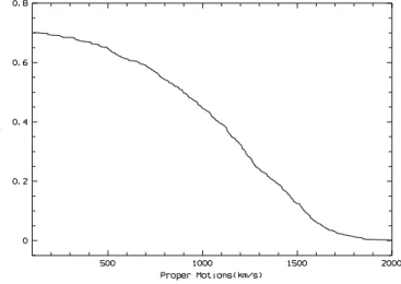
(corrected for richness, background and statistical effects) is due to peculiar motions, we can deduce the probability to have an error if we assume that the remaining dispersion is lower than (σ2obs-σ2)1/2. We are thus able to give an upper limit for the amplitude of the cluster radial peculiar motions at a given con-fidence level. We compute these equivalent upper peculiar mo-tions by adopting a mean velocity of 20000 km.s−1(see Fig. 7).
If we consider for example a risk of 45% for P(σstat≤σ), we
give a dispersion of 0.11 magnitude equivalent to peculiar mo-tions within an amplitude of 1000 km.s−1(0.09 magnitude or
800 km.s−1without A0087). With a conservative risk of 10%,
we predict a dispersion of 0.17 magnitude equivalent to pecu-liar motions less than 1500 km.s−1 (0.13 magnitude or 1200
km.s−1without A0087).
4.2.1. Analysis
We have reduced the dispersion of the mn-cz relation by
sub-tracting the background galaxies and by modeling the effects of the cluster population. We determine in this way an upper limit for the dispersion due to peculiar velocities. We deduce
Fig. 7. Probability of having peculiar velocities greater than a given
value (we have adopted a mean velocity of 20000 km.s−1 for our
clusters). This curve is shifted by about -300 km.s−1 if we remove
A0087 from the sample.
that this maximal dispersion is somewhat larger than the value of Bahcall & Oh (1996). They found a risk inferior to 5% to have clusters of galaxies with a random peculiar velocity greater than 600 km.s−1. However, their studied clusters (and groups) have
a recession velocity less than 10000 km.s−1and the equivalent
magnitude dispersion is similar to our result.
Several other studies have analyzed the proper motions of the nearby clusters in the CMB frame: Lauer & Postman (1994), Colless (1995) or more recently Hudson & Ebeling (1997). They use the slope of the brightness profiles of cD galaxies as distance indicator. The Lauer & Postman (respectively Colless and Hud-son & Ebeling) distance indicator precision is 0.24 magnitude (respectively 0.24 and 0.41 magnitude). This is similar to our precision.
We can also directly compare our dispersion of 0.21 mag-nitude (without statistical correction, see above) with the value of Perlmutter et al. (1997). They have used a sub-sample of 28 distant type Ia supernovae to constrain the cosmological param-eters, and they obtain a dispersion of 0.19 magnitude, very con-sistent with our value. Finally, we have similar values (slightly greater) for the peculiar velocities than in A98a with almost the same sample.
5. Conclusion
We have readressed the question of the determination of a dis-tance indicator by using as standard candle the nth ranked galaxy.
In order to correct the magnitudes for different factors, we have addressed the question of the universality of the Luminos-ity Function for rich clusters of galaxies. We have constructed a CCLF by using 28 rich clusters in the magnitude range [-21;-17]. The fit of a Schechter model gives α=-1.50±0.11 and Mbj∗=-19.91±0.21 in good agreement with other literature
re-sults. This function is found to be universal for these clusters, consistent with the L97 study.
Table 1. Parameters for the 28 used clusters. Col.(1) cluster name,
col.(2) m5 without any corrections, col.(3) distance indicatorµ
cor-rected for richness and background galaxies and calculated with m15,
col.(4) 5.×log(cz)
cluster name m5 µ 5log(cz)
0013 17.64 37.18 22.25 0087 16.88 35.24 21.09 0119 15.88 35.28 20.60 0151 17.76 35.91 21.01 0168 16.23 35.63 20.65 0367 17.05 37.14 22.18 0514 16.86 36.08 21.67 1069 15.92 36.72 21.45 2362 17.25 35.96 21.31 2480 17.09 36.70 21.67 2644 17.72 36.47 21.58 2734 16.77 36.25 21.35 2764 16.49 36.19 21.64 2799 16.95 36.51 21.38 2800 16.53 36.40 21.42 2854 17.33 36.22 21.31 2911 17.39 36.84 21.93 2923 17.66 36.51 21.64 3111 16.80 36.77 21.85 3112 16.23 37.06 21.76 3122 16.84 36.46 21.42 3141 16.40 37.39 22.49 3158 16.41 36.28 21.24 3202 16.91 36.78 21.58 3733 16.94 35.36 20.34 3764 16.84 36.68 21.79 3825 16.79 37.09 21.76 3827 17.29 37.21 22.34
We have found that the uncorrected distance indicator mn
is more efficient for the first ranks n. With n=5, we observe a dispersion of about 0.6 magnitude, too large however to derive correct peculiar velocities.
We then use the CCLF to model the effect of the cluster richness on mnin order to have a better precision and to better
constrain the cluster peculiar velocities. We correct first for the richness effect and second for the background galaxies subtrac-tion. This allows to reduce the dispersion to 0.254 magnitude (0.210 without A0087). If we assume that this error is only due to peculiar velocities, they are 2300 km.s−1(1900 km.s−1
with-out A0087) for a cluster at 20000 km.s−1. However, a large part
of this dispersion is due to statistical effects. By using exten-sive simulations, we give the probability distribution to have a peculiar motion lower than a given value. For example, with a risk of 10%, we predict a value of 1500 km.s−1(1200 km.s−1
without A0087).
These results agree well with local estimates. We have also consistent results with A98a who used the Fundamental Plane for the same clusters as used here.
38 S. Rauzy et al.: Cluster luminosity function and nthranked magnitude as a distance indicator,
Acknowledgements. We wish to thank Dr. J. Lequeux and R. Malina
for a careful reading of the manuscript.
References
Abell G.O., Corwin H.G., Olowin R.P., 1989, ApJS 70, 1 (ACO) Adami C., Mazure M., Biviano A., Katgert P., Rhee G., 1997, A&A
331, 439 (A98a)
Adami C., Mazure M., Katgert P., Biviano A., 1998, A&A submitted (A98b)
Bahcall N.A., Oh S.P., 1996, ApJ 462, L49 Beers T.C., Tonry J.L., 1986, ApJ 300, 557
Bernstein G.M., Nichol R., Tyson J.A., Ulmer M.P., Wittman D., 1995, AJ 110, 1507
Biviano A., Katgert P., Mazure A., et al., 1996, A&A 321, 84 Burstein D., Heiles C., 1982, AJ 1165, 87
Colless M., 1995, AJ 109, 1937 Colless M., 1989, MNRAS 237, 799
de Theije P.A.M., Katgert P., 1998, A&A submitted (paper VI) Durret F., Forman W., Gerbal D., Jones C., Vikhlinin A., 1998, A&A
accepted
Feldman H.A., Watkins R., 1994, ApJ 430, 17
Heydon-Dumbleton N.H., Collins C.A., MacGillivray H.T., 1989, MN-RAS 238, 379
Hudson M., Ebeling H., 1997, ApJ 479, 621
Isobe T., Feigelsen E.D., Akritas M.G., Babu G.J., 1990, ApJ 364, 104 Jones B.J.T., Mazure A., 1993, to app. in Measuring, Mapping and
Modelling the Universe (http : //www.tac.dk/bjones/)
Katgert P., Mazure A., den Hartog R., et al., 1998, A&A accepted (K98) Katgert P., Mazure A., Perea J., et al., 1996, A&A 310, 8
Lauer T.R., Postman M., 1994, ApJ 425, 418
Lobo C., Biviano A., Durret F., et al., 1996, A&A 317, 385
Lubin P., Villela T., 1986, in Galaxy Distances and Deviations from Universal Expansion, ed. B.F. Madore and R.B. Tully, Dordrecht (Reidel p.169)
Lumsden S.L., Collins M.A., Nichol R.C., Eke V.R., Guzzo L., 1997, MNRAS 290, 119 (L97)
Mazure A., Katgert P., den Hartog R., et al., 1996, A&A 310, 31 Merrifield M.R., Kent S.M., 1989, AJ 98, 351
Perlmutter S., Gabi S., Goldhaber G., et al., 1997, ApJ 483, 565 Schaeffer R., Maurogordato S., Cappi A., Bernardeau F., 1993,
MN-RAS 263, L21
Schechter P.L., 1976, ApJ 203, 297 Trentham N., 1998, Astro-ph (9804013)
Valotto C.A., Nicotra M.A., Muriel H., Lambas D.G., 1997, ApJ 479, 90 (V97)
![Fig. 3. CCLF’s issued from the three radial bins: [0,2] r c (filled), [2,3.5]](https://thumb-eu.123doks.com/thumbv2/123doknet/14576892.728613/5.918.65.442.62.311/fig-cclf-s-issued-radial-bins-r-filled.webp)