HAL Id: hal-02125436
https://hal.archives-ouvertes.fr/hal-02125436
Submitted on 3 Dec 2019
HAL is a multi-disciplinary open access
archive for the deposit and dissemination of
sci-entific research documents, whether they are
pub-lished or not. The documents may come from
teaching and research institutions in France or
abroad, or from public or private research centers.
L’archive ouverte pluridisciplinaire HAL, est
destinée au dépôt et à la diffusion de documents
scientifiques de niveau recherche, publiés ou non,
émanant des établissements d’enseignement et de
recherche français ou étrangers, des laboratoires
publics ou privés.
Distributed under a Creative Commons Attribution - NonCommercial - NoDerivatives| 4.0
MRAS Scheme
Youssef Agrebi Zorgani, Mabrouk Jouili, Yassine Koubaa, Mohamed Boussak
To cite this version:
Youssef Agrebi Zorgani, Mabrouk Jouili, Yassine Koubaa, Mohamed Boussak. A Very-Low-Speed
Sensorless Control Induction Motor Drive with Online Rotor Resistance Tuning by Using MRAS
Scheme. Power Electronics and Drives, 2018, 4 (1), pp.171-186. �10.2478/pead-2018-0021�.
�hal-02125436�
Power Electronics and Drives
Research Article
1 Laboratory of Sciences and Techniques of Automatic Control & Computer Engineering (Lab-STA),
National School of Engineering of Sfax, University of Sfax, Postal Box 1173, 3038 Sfax, Tunisia
2 Laboratoire des Sciences de l’Information et des Systèmes (LSIS), UMR CNRS 7296 - Ecole Centrale
de Marseille (ECM), Marseille, France
Youssef Agrebi Zorgani
1,2, Mabrouk Jouili
1, Yassine Koubaa
1, Mohamed Boussak
2A Very-Low-Speed Sensorless Control Induction
Motor Drive with Online Rotor Resistance Tuning
by Using MRAS Scheme
1. Introduction
Indirect flux-oriented control (FOC) techniques are now widely used for the control of induction motor drives in high- performance applications. For the stator-flux-oriented control (SFOC) induction motor drive, the rotor position – using an incremental optical or magnetic encoder sensor placed on the shaft – and information of the current’s components are continuously required (Boussak and Jarray, 2006). However, the rotor position sensor leads to reduced reliability and requires additional cabling and space on the shaft. It also increases cost, weight and susceptibility to noise.
To overcome these problems, the use of sensorless control without a mechanical sensor is an attractive solution. Actually, advanced research works focus on the SFOC induction motor drive approach, which independently controls both the torque and the flux without a mechanical sensor. These investigations have been performed during the past few years. They are aimed at the development of the sensorless SFOC featuring a dynamic behaviour comparable or similar to the drives equipped with a mechanical sensor on the shaft. Nowadays, with the progress of power electronics, microcontrollers and digital signal processors (DSPs), sensorless alternating current (AC) motor drives without a mechanical sensor are becoming real in high-performance industrial applications.
Received September 02, 2018; Accepted October 08, 2018
Keywords: Induction motor • Stator flux orientation model • Model reference adaptive system (MRAS) • Rotor speed and resistance estimation • Programmable cascaded low-pass filters (PCLPF)
Abstract: A sensorless indirect stator-flux-oriented control (ISFOC) induction motor drive at very low frequencies is presented herein. The model reference adaptive system (MRAS) scheme is used to estimate the speed and the rotor resistance simultaneously. However, the error between the reference and the adjustable models, which are developed in the stationary stator reference frame, is used to drive a suitable adaptation mechanism that generates the estimates of speed and the rotor resistance from the stator voltage and the machine current measurements. The stator flux components in the stationary reference frame are estimated through a pure integration of the back electro-motive force (EMF) of the machine. When the machine is operated at low speed, the pure integration of the back EMF introduces an error in flux estimation which affects the performance torque and speed control. To overcome this problem, pure integration is replaced with a programmable cascaded low-pass filter (PCLPF). The stability analysis method of the MRAS estimator is verified in order to show the robustness of the rotor resistance variations. Experimental results are presented to prove the effectiveness and validity of the proposed scheme of sensorless ISFOC induction motor drive.
Several methods for the sensorless SFOC induction motor drive are presented in the literature, such as the observer-based techniques of artificial neural networks (ANNs) (Nassar and Khoei, 2015; Verma et al., 2014), Luenberger observers (LOs) (Propovic et al., 2014), extended Kalman filter (EKF) observers (Ben ammar et al., 1991; Barut et al., 2012), slidingmode observers (SMOs) (Comanescu, 2015) and fuzzy logic (Abbou et al., 2012; Zahraoui et al., 2016). Most of the sensorless SFOC induction motor drive systems are sensitive to inaccuracies, such as the stator and the rotor resistance. Therefore, they should be estimated online in order to obtain robust control (Hadj Saïd et al., 2011).
In previous works (Agrebi et al., 2007; Agrebi-Zorgani et al., 2010; Dybkowski, 2018; Dybkowski and Orlowska-Kowalska, 2013; Zaki Diab et al., 2016), the MRAS scheme has been used to estimate the speed and the rotor resistance. This control method is presented for the sensorless indirect stator-flux-oriented control (ISFOC) induction motor (IM) drive. Again, a detailed description of the proposed technique and its usefulness are given. More importantly, in a previous study (Agrebi-Zorgani et al., 2010), the performances of simultaneous estimation algorithms are tested by simulations.
This paper investigates the MRAS scheme using only stator current and voltage measurements to
simultaneously
estimate the speed and the rotor resistance at a very low speed. Initially, a strategy of the SFOC induction motor drive is presented. Then, a theoretical study of the proposed algorithm is given even at low speeds. Afterwards, the stability of the two MRAS estimators is studied. Finally, the proposed method is confirmed with experimental studies, which are conducted on a test bench provided with a chart of real-time control of the type dSpace DS1104 real-time controller board.
This paper is structured in five sections including the first section ‘Introduction’, as follows. In Section 2, the model of the stator flux orientation is presented. The procedure design proposed for the simultaneous estimation of speed and rotor resistance using the MRAS speed estimation scheme is described in Section 3. Experimental results are shown in Section 4. Finally, a conclusion is drawn in Section 5.
2. IM model in the stator-flux-oriented frame
By using the stator flux, the dynamic IM model in a synchronous reference frame is given by Equation 1. Speed control can be ensured by a proportional integral (PI) controller, which cancels the static error and improves the dynamic performances of the closed loop speed. Therefore, we choose an integral proportional (IP) controller, which is different from the PI controller by the fact that it does not present a zero in the closed loop transfer function and offers, thus, a better stability (Jarray, 2000).
The control of the components d-q currents is ensured by a PI controller, in order to reduce the static error and improve the dynamic performances of the current loops.
φ φ ω ω ω στ ω σ σ τ σ τ σ ω ω σ στ ω σ τ σ τ σ φ φ ω σ σ = − − − + − − − + − − + − d dt d dt di dt di dt d dt R R L L L L n J i n J i f J i i L L J v v n T 0 0 0 0 0 0 1 1 0 1 1 0 0 0 1 0 0 0 1 0 1 0 0 0 1 0 0 0 1 ds qs ds qs s s s s r s s s r s r sl s r s sl s r s r p qs p ds ds qs ds qs s s ds qs p l 2 2 (1) with: ωsl=ω ωs− , τ = L R r r r , τ = L R s s s and σ = − M L L 1 s r 2 .
3. Description of the MRAS technique
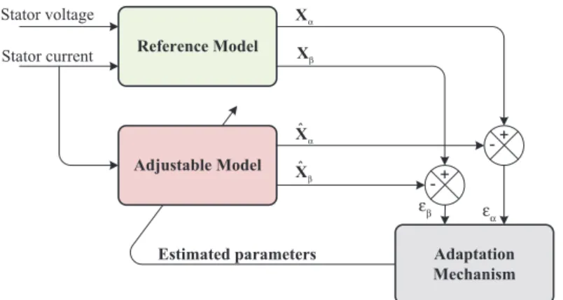
The principle of the MRAS estimation technique focuses on the determination of two models: reference and adjustable ones (Fig. 1). The reference and adjustable models, developed in stationary stator reference frame, are used in the MRAS scheme to estimate rotor speed and rotor resistance from measured terminal voltages and currents.
The general idea behind MRAS is to create a closed loop controller with parameters that can be updated to change the response of the system. The output of the reference model is compared with an adjustable observer model. The error is fed into an adaptation mechanism, which is designed to ensure the stability of the MRAS (Agrebi et al., 2007; Agrebi-Zorgani et al., 2010). Thus, the update of the control parameters must be performed based on this error. This strategy allows the parameters to converge to ideal values (Agrebi et al., 2007; Agrebi-Zorgani et al., 2010, 2016).
Reference Model Adjustable Model Ada εβ ptation Mechanism + -+ -Stator voltage Stator current Xα Xβ ˆXα ˆXβ εα Estimated parameters
Fig. 1. Synopsis of the MRAS method
3.1 Simultaneous speed and rotor resistance estimation
In order to estimate the rotor speed ω and the rotor resistance Rr, it is wise to use induction motor model in a
stationary reference frame (α, b). This transformation does not call upon the position of the rotor, which is estimated by the MRAS scheme (Agrebi et al., 2007; Kalovsky et al., 2016).
The stator voltages can be described by the following equation:
φ φ = + = + α α α β β β v R i d dt v R i d dt s s s s s s s s (2)
The rotor voltages can be described by the following equation:
φ ωφ φ ωφ = + + = + − α α β β β α R i d dt R i d dt 0 0 r r r r r r r r (3) with φ φ = + = + α α α β β β L i Mi L i Mi r r r s r r r s (4)
Equations (3) and (4) are rewritten under the following new form: φ ω φ ω φ φ = − − + + = − − + α β α β α β α β L Di Ei D L Ei L Di L D 0 0 s s s s r s s s s r s s (5) where D R= r+p Lσ r and E=σL Ls rω.
By using Equations (2) and (3), we can identify the speed ω and the rotor resistance Rr. Then, we try to represent
the components of the stationary reference frame stator flux (fαs,fbs) in terms of accessible stator variables which
are the stator currents (iαs,ibs) and stator voltages (vαs,vbs). Consequently, two independent stator flux estimators are
built. The first is obtained by integrating the Equation (2), the second flux estimators appear by using Equation (5). It is noticed well that Equation (2) does not contain the parameters ω and Rr. Therefore, it can be considered as
a reference model of the IM. However, Equation (5) includes the parameters ω and Rr, and it is considered as an
adjustable model.
The error between the states of the two models, given by Equation (6), is used to drive a suitable adaptation mechanism that generates the estimation of ω and Rr, for the adjustable model. Since the expression of the feedback
block W, which is presented in Equation (7), is different for the speed estimation and rotor estimation, two adaptation mechanisms come up:
– Adaptation mechanism 1 – Adaptation mechanism 2 ε φ φ ε φ φ = − = − α α α β β β ˆ ˆ s s s s (6)
Equation (6) can be presented as follows (Agrebi et al., 2007; Agrebi-Zorgani et al., 2010):
ε = ε +
p[ ] [ ][ ] [ ]A W (7)
where W is the feedback block, which establishes the input of the linear block. – For the speed estimation
τ ω ω τ = − − − A 1 1 r r and φ σ φ σ
(
ω ω)
= = − + − − β β α α W W Lsi Lsi ˆ ˆ ˆ s s s s 1Equations (6) and (7) constitute a non-linear feedback system represented by Fig. 2. Indeed, this system can be schematised by a linear block described by the transfer matrix H p( ) ( [ ] [ ])= p I − A −1 and a non-linear part of the input e(t) and the output W(e,t).
– For the rotor resistance estimation
ω ω = − − − A R L R L r r r r and φ φ
(
)
= = − + − + − α α β β W W L i L L i L R R ˆ ˆ ˆ s s s r s s s r r r 2Equations (6) and (7) constitute a non-linear feedback system represented by Fig. 3. Indeed, this system can be schematised by a linear block described by the transfer matrix H p( ) ( [ ] [ ])= p I − A −1 and a non-linear part of the input e(t) and the output W(e,t).
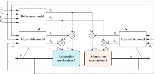
The estimation technique involves use of the adaptation Mechanism 1 to estimate the rotor speed. Subsequently, the adaptation Mechanism 2 is used to estimate the rotor resistance Fig. 4.
The values of speed and rotor resistance are provided at each calculation step for speed and current regulators of the control block.
Fig. 4. Structure of the simultaneous speed and rotor resistance estimation by MRAS technique
1/P [A] Adaptation mechanism + + + + -0 Li ne ar b lo ck N on -li ne ar b lo ck s s s s s s L i L i W ˆ s i is
Fig. 2. Non-linear feedback system for speed estimation
The asymptotic operation of the adaptation mechanism is fulfilled by a simplified condition, which is [ ( )]ε ∞ T =0. To be regarded as hyper-stable, the system of negative feedback must satisfy the inequality of Popov (Schauder, 1992):
∫
t[ ] [ ]εT W dt≥ −γ20
1
for all t1 ≥0 (8)
where g is a negative constant.
3.2 Speed adaptation mechanism
The general structure of the adaptation Mechanism 1 shows that the estimated speed ωˆ is a function of the error [e]. Indeed, it can be written down as follows:
∫
ω= + = ε + ε pA A A dt A ˆ 1 1 2 t 1([ ])1 ([ ]) 0 2 1 0 (9)where A1 and A2 are non-linear function of eα1, and eb1, respectively.
By using the expression of W, Equation (8) becomes equivalent to the following:
∫
ε(
−φ +σ) (
+ε φ −σ)
ω ω γ − ≥ − α ˆβs Lsiβs β ˆαs Lsiαs ( ˆ )dt t 1 1 2 0 0 (10) with: φ φ φ φ ε ε σ φ φ φ φ ε ε σ = − − − = − − − β α α β α β β α β α α β α β β α A K i i L A K i i L ( ˆ ˆ ( ) ( ˆ ˆ ( ) s s s s s s s s s s s s s s 1 2 1 1 2 1 1 1where K1 and K2 are called adaptation gains, which are constants and positive.
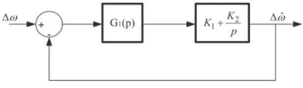
Equation (9) is built around a PI regulator. Fig. 5 represents the result of the synthesis of the speed regulator (Agrebi et al., 2007; Agrebi-Zorgani et al., 2010).
Fig. 5. Synthesis of the speed corrector
To study the dynamic response of the speed estimated by the MRAS method, it is necessary to linearise the stator and the rotor equations around an operating point. Thus, the error variation e is expressed as follows (Agrebi et al., 2007; Agrebi-Zorgani et al., 2010): ε φ φ φ φ φ φ φ φ φ φ φ φ ∆ = ∆ + ∆ + − ∆ + ∆ + α α β β α β α α β β α β ˆ ˆ ˆ ˆ ˆ ˆ s s s s s s s s s s s s 0 0 0 0 0 2 0 2 0 0 0 0 0 2 0 2 (11)
The transfer function representing the variation ratio De compared with ∆ ˆω is written as follows:
ε ω β φ β ω ∆ ∆ = + + + ω
(
)
(
)
(
)
∆ → p p ˆ rr 0 2 2 2 0 (12)In a steady operation, one will have the following equalities:
Then, by neglecting the effect of the slip pulses ωsl, the transfer function of G1(p) will be as follows: G p p ( ) 1 r 1 0 2 φ τ = + (13)
Hence, the transfer function of the direct chains is written as in Eq. (14):
φ τ
( )
=(
+)
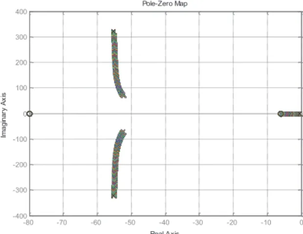
+ F p K p K p 1 p r 02 1 2 (14)We chose an optimal damping coefficient (x = 0.7) to determine the parameters K1 and K2 of the PI corrector. The transfer function F(p) of the speed estimator using the MRAS scheme is influenced by the induction motor parameters, the PI regulator coefficients K1 and K2, and the real speed. To highlight the influence of the real speed on the stability of the estimator, the place of the zeroes and the poles for various values of ω are presented.
For a rotor speed variation in the interval from 0 to 314 rad/s, the MRAS estimator poles’ locations are shown in Fig. 6. -80 -70 -60 -50 -40 -30 -20 -10 0 -400 -300 -200 -100 0 100 200 300 400 Pole-Zero Map Real Axis six A yr ani ga mI
Fig. 6. Evolution of the MRAS estimator poles and zeros according to the speed
We note that the variation speed does not affect the stability of the system.
3.3 Rotor resistance adaptation mechanism
The general structure of the adaptation Mechanism 2 shows that the estimate of the rotor resistance Rˆr is a function of the error [e]. Indeed, it is given by the following expression (Agrebi et al., 2007; Agrebi-Zorgani et al., 2010):
∫
ε ε = + = + R pA A A dt A ˆr 1 t ([ ]) ([ ]) 3 4 0 3 2 4 2 0 (15)where A3 and A4 are non-linear functions of eα2 and eb2, respectively.
Using the expression of W2, Equation (8) becomes equivalent to the following expression:
L i L L i L R R dt ˆ s s s ˆ ˆ r s s s r r r t 2 2 2 0 0
∫
ε −φ + ε φ(
)
γ + − + − ≥ − α α α β β β (16)with: φ ε φ ε φ ε φ ε = − + +− + = − + +− + α α α β β β α α α β β β A K L i L L i L A K L i L L i L ˆ ˆ ˆ ˆ s s s r s s s r s s s r s s s r 3 4 2 2 4 3 2 2
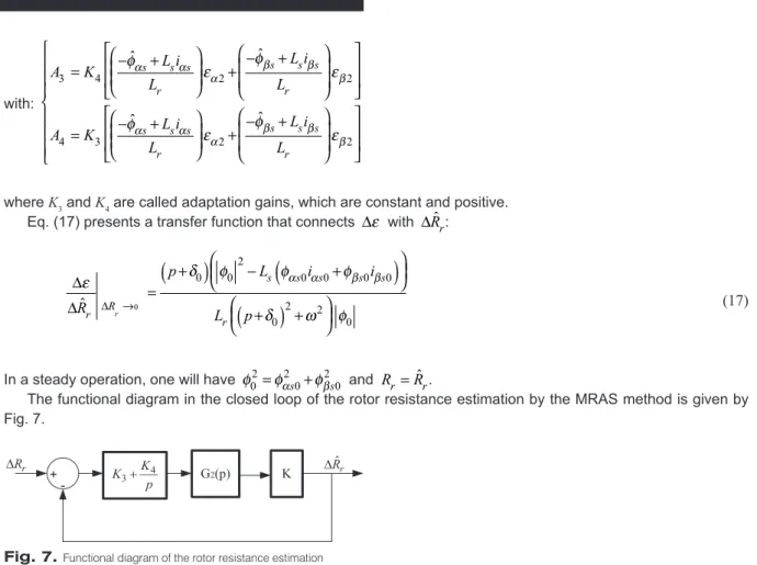
where K3 and K4 are called adaptation gains, which are constant and positive. Eq. (17) presents a transfer function that connects ∆ε with ∆Rˆr:
ε δ φ φ φ δ ω φ
(
)
(
)
(
)
∆ ∆ = + − + + + α α β β ∆ → R p L i i L p ˆ r R s s s s s r 0 0 2 0 0 0 0 0 2 2 0 r 0 (17)In a steady operation, one will have φ02=φα2s0+φβ2s0 and Rr =Rˆr.
The functional diagram in the closed loop of the rotor resistance estimation by the MRAS method is given by Fig. 7.
Fig. 7. Functional diagram of the rotor resistance estimation
In this functional diagram, the expression of K is given by Eq. (18) (Agrebi-Zorgani et al., 2010):
φ φ φ φ
(
)
= − α α + β β K L i i L s s s s s r 0 2 0 0 0 0 0 (18) ω = + + + G p p R L p R L ( ) r r r r 2 2 2 (19)Two complex poles (p1 and p2) are presented in the transfer function G2(p):
ω = − + p R Lrr j 1 (20) ω = − − p R Lrr j 2 (21)
The real part of the two complex poles p1 and p2 are negative. Thus, the stability of the function is confirmed. Again, the use of a PI regulator enabled us to obtain a fast convergence and a null static error in the steady state operation.
-300 -250 -200 -150 -100 -50 0 50 -200 -150 -100 -50 0 50 100 150 200 Root Locus Real Axis six A yr ani ga mI
Fig. 8. Locations of poles and zeroes of G2(p)
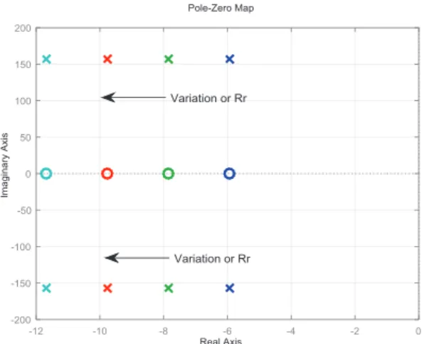
The layout of the roots locations related to the transfer function G2(p) for 157 rad/s is given in Fig. 8, which characterises the dynamics of the control system. In fact, this function has two poles and a zero, which are all located in the left half-plan of the complex plan. The poles p1 and p2 are complex conjugate poles and located at -5.94 ± 157j. Their locations characterise the dynamics of the system. Thus, to ensure a good tracking performance and a fast transient response, the zero placement of the PI regulator must be located on the real axis at -5.94 (located on the left half-plan). Consequently, K3 must be taken of a rather large value and the ratio K4/K3 must be equal to the negative real part of the complex poles of the systems (Zaky, 2011, 2012) (K3 = 500 and K4/K3 = 5.94). This allows us to have an error of the rotor resistance that decreases the fast exponential form with time without oscillation (over-oscillation or under-oscillation).
Fig. 9. Locations of poles and zeroes of G2(p) for different values of Rr
The zero location of the controller PI (K4/K3) can be selected for the value of the rotor resistance given by Fig. 9. In other words, this figure shows the location of the poles of G2(p) with various values of Rr.
3.4 Stator flux estimation
In the reference model, and according to system Equation (2), the two fluxes fαs and fbs are determined through
the integration of the back electromotive force (EMF) of the machine. The estimated flux is obtained by a pure integration and can cause significant problems, in particular, at low frequency due to the noise sensor, the voltage shift (direct current [DC] offset), and the uncertain parameters. In order to overcome these problems, the pure integrator is replaced with a low-pass filter (LPF) (Ghaderi and Hanamoto, 2011). In this paper, we propose to replace the pure integrator with a programmable cascaded low pass filter (PCLPF). This approach has already been proposed to control the IM without a mechanical sensor (Ghaderi et al., 2006). Indeed, a PCLPF includes a few
blocks of these filters. Each block decreases the effect of the voltage shift (DC offset). In one PCLPF, their gains as well as their cut-off frequencies are given according to the stator frequency.
Accordingly, two methods are proposed. In the first method, which is called a modified programmable cascaded low-pass filters (MPCLPF), the estimate precision is improved by eliminating the gain in the calculation phase. In the second method, which is called the extended PCLPF (EPCLPF) (Ghaderi et al., 2007), the estimator behaviour is modified by the elimination of the gain G in the calculation phase and the extension low-pass filter stages (LPF stages). This method can be applied only to the area of very low speed.
3.4.1 Modified programmable cascaded low-pass filter (MPCLPF)
To calculate the phase, qs, fbs(p) must be divided by fαs(p). However, in the terms (fαs(p) and fbs(p)), G is a common
factor, so it can be eliminated by simplification. This approach is illustrated below: H’(p) which is defined as the transfer function of MPCLPF is given by Equation (22).
τ = ⋅ + H p p ( ) 1 1 ' 3 (22) F pα( )=
(
vαs( )p R i p H p− s sα ( ))
'( ) (23) F pβ( )=(
vβs( )p R i p H p− s sβ ( ))
'( ) (24) F t F t F p F p tan ( ) ( ) tan ( ) ( ) s 1 1 1 1 θ(
)
(
)
= = β α β α − − − − (25)3.4.2 Extended programmable cascaded low-pass filter (EPCLPF)
As previously mentioned, the reduction of the continuous voltage shift (DC offset) is an effective means for the sensorless control in the low-speed region (Ghaderi et al., 2007). As the output depends on the gain of the PCLPF, this last should be reduced. Here, it is necessary to take the relation between the amplitude of the gain and the order of the PCLPF into account. For a number of N LPF stages presented in Fig. 10, the time constant of the filters, the gain and the transfer function are calculated as follows:
τ ω π = ⋅ n 1 tan 2 e (26) ω ω τ = + G 1 1 ( ) e e n 2 (27)
By using the expression (26), Equation (27) becomes as follows:
ω π = + ⋅ G n 1 1 tan 2 e n 2 (28) τ = ⋅ + H p G p ( ) 1 1 n (29)
Fig. 10. Diagram of N floors of programmable low-flow filter.
4. Experimental results
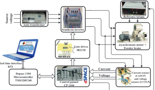
To validate the performance of estimation of the simultaneous parameters, a prototype implementation of the sensorless ISFOC of an induction motor drive was carried out. Experimental tests were done based on the estimation scheme for sensorless ISFOC of an induction motor, which is proposed in Fig. 11. As a matter of fact, the experimentation has been achieved by using MatLab-Simulink and dSpace DS1104 real-time controller board. The experimental set-up is composed of squirrel-cage IM a 3 kW (Table. 1), a pulse-width modulation (PWM) signal to control the power modules generated by dSpace system, a voltage source inverter (VSI) and a load generated through a magnetic power brake coupled with the three-phase induction motor. The DC link voltage, stator phase currents and voltages are measured by Hall-type sensors.
In order to demonstrate the effectiveness and the robustness of the proposed method, we try out the system for the following operating modes:
• A speed reference of 15 rpm, before applying a rated load torque (20 Nm) at t = 7 s, and cancelling that at
t = 13 s.
• A speed reference of 15 rpm by inverting the rotation direction at the instant t = 9.5 s.
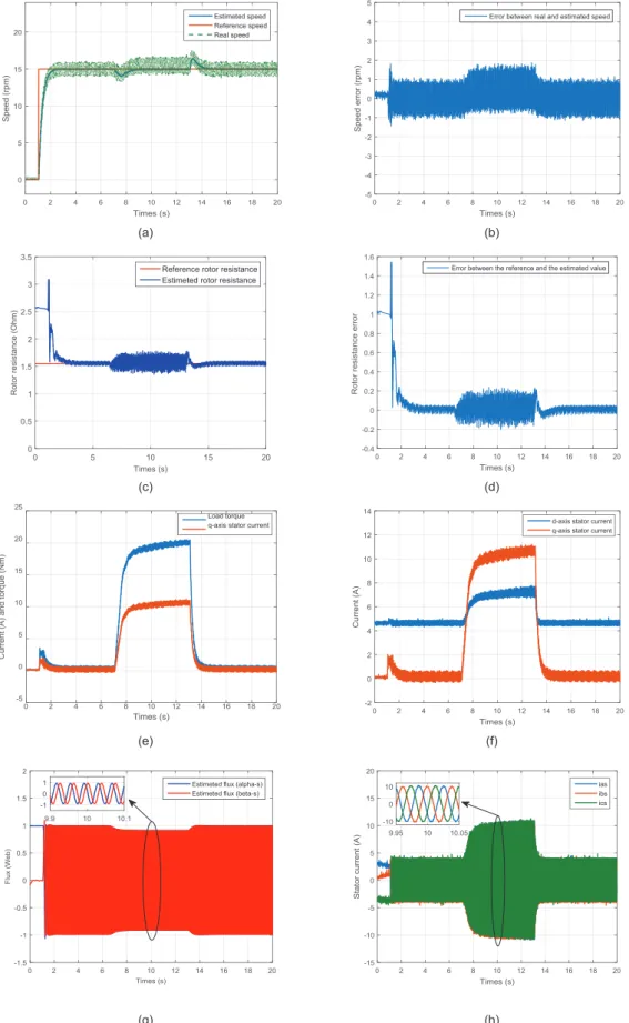
• The first case: a preset speed of 15 rpm, followed by the application of a load torque at t = 7 s, and the abolition of the latter at t = 13 s.
The experimental tests, illustrated by Fig. 12(a), show that the estimated speed and the actual speed converge to that of the reference. The error between the estimated and the actual sizes is presented by Fig. 12(b), and it does not exceed 2 rpm in the steady state. This value of the error is important because of the sensor reliability, which is used to measure the actual speed. However, the velocity sensor used in our application is an incremental encoder with 1,024 pulses per revolution. For a low-speed operation, the velocity precision decreases. Consequently, the error between the real and the estimated rotor speeds increases.
Fig. 12(c) shows the curves of the estimated rotor resistance Rr and those of the reference. The convergence of the estimated size of Rr to its reference is proved by Fig. 12(d), representing the error between the estimated and the reference sizes.
Furthermore, Fig. 12(e) confirms the proportionality between the q-axis stator current and the electromagnetic torque. Knowing that, the measurement of the stator current is used to estimate the electromagnetic torque. The fluxes fαs and fbs are presented in Fig. 12(g); it shows that they are in a quadratic phase. The curves of the
d-axis and q-axis stator currents are given by Fig. 12(f). Finally, the stator currents ias, ibs and ics are presented
in Fig. 12(h).
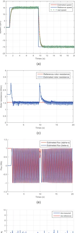
• The second case: a pre-set speed of 15 rpm by inverting the rotation direction at the moment t = 9.5 s.
In Fig. 13, the sensorless speed reversal tests are carried out to show the robustness of the proposed scheme for the sensorless ISFOC induction motor drive and the behaviours of the motor during speed transients. In Fig. 13(a), the speed reversal test is performed, from which one observes that the speed estimation and the actual speed converge to that of the reference. The error between the estimated and the actual sizes is presented in Fig. 13(b), and it does not exceed 2 rpm in the steady state. Note that, this error can be <1 rpm if the actual value is measured by a more precise incremental encoder.
Fig. 13(c) shows the curves of the estimated rotor resistance and those of the reference. The convergence of the estimated size of rotor resistance Rr to its reference is proved by Fig. 13(d), representing the error between the estimated and the reference values, while Fig. 13(e) indicates that even for low speeds the fluxes fαs and fβs are in a quadratic phase. However, the convergence of the estimated size of iqs stator current to its reference is proved by the Fig. 13(f), the same can be said for Fig. 13(g), which presents the ids stator current. Finally, Fig. 13(h) shows the stator currents ias, ibs and ics.
These results confirm that the control scheme, even at low speeds, has a good robustness and a good tracking performance.
5. Conclusion
In this paper, a very low rotor speed estimation of the speed sensorless control of the IM with online rotor resistance tuning has been designed. The technique of this simultaneous estimation is based on the MRAS method. The analysed closed-loop stability of the presented method has also been proved though the Lyapunov stability theory. The online rotor resistance estimation scheme has been proposed to be updated in the adjustable model in each computational step, which guarantees the stability of the drive and ensures the accuracy of sensorless speed control. The experimental results show that the rotor resistance is sensitive to the load variation. More importantly, the validity of the proposed sensorless ISFOC of the induction motor drive was proven by experiments for a very
Table 1. Induction motor parameters
Specification Parameters Rated power 3 kW Rs 2.3 Ω
Rated voltage 380 V Rr 1.55 Ω
Rated current 6.6 A Ls, Lr 0.261 H
Rated frequency 50 Hz LM 0.245 H
Number of pole pair 2 J 0.02 kg.m2
(a) (b)
(c) (d)
(e) (f)
(g) (h)
(a) (b)
(c) (d)
(e) (f)
(g) (h)
low speed. Thus, all experimental results confirm the high dynamic performances of the developed drive system and show the validity of the proposed method.
Nomenclature
vds, vqs, ids, iqs fds, fqs fαs, fbs Rr, Rs Lr, Ls M np ωs, ω ωsl Te, Tl J f ts, tr kvi, kvp kip, kip s ^, * p d dt =d, q- axis stator voltage and current components
d, q- axis stator flux components
α, b- axis stator flux components Rotor and stator resistances Rotor and stator self-inductances Mutual inductance
Number of pole pairs
Synchronous and rotor angular speeds Slip angular speed (ωs – ω)
Electromagnetic and load torques Moment of inertia
Friction constant
Stator and rotor time constants
Integral an proportional gains of the IP speed controller Integral and proportional gains of the PI current controller Total leakage constant
Estimated and reference values Differential operator
References
Abbou, A., Nasser, T., Mahmoudi, H., Akherraz, M. and Essadki, A. (2012). dSPACE IFOC Fuzzy Logic Controller Implementation for Induction Motor Drive. Journal of Electrical Systems, 8(3), pp. 317–327.
Agrebi, Y., Triki, M., Koubaa, Y. and Boussak, M. (2007). Rotor Speed Estimation for Indirect Stator Flux Oriented Induction Motor Drive Based on MRAS Scheme. Journal of Electrical Systems, 3(3), pp. 131–143.
Agrebi-Zorgani, Y., Koubaa, Y. and Boussak, M. (2010). Simultaneous Estimation of Speed and Rotor Resistance in Sensorless ISFOC Induction Motor Drive Based on MRAS Scheme. IEEE International
Conference on Electrical Machines ICEM, Rome,
6-8 September 2010, IEEE, pp. 1–6.
Agrebi-Zorgani, Y,. Koubaa, Y. and Boussak, M. (2016). MRAS State Estimator for Speed Sensorless ISFOC Induction Motor Drives with Luenberger Load Torque Estimation. ISA Transactions, 61, pp. 308–317.
Barut, M., Demir, R., Zerdali. E. and Inan, R. (2012). Real Time Implementation of Bi Input Extended Kalman Filter Based Estimator for Speed
Sensorless Induction Motor. Transactions on
Industrial Electronics, 59(11), pp. 4197–4206.
Ben Ammar, F., Pietrzak-David, M., De Fornel, B. and Merzaian, A. (1991). Field oriented control of high-power motor drives by Kalman filter flux observation. In: Proceeding, EPE’91, Firenze, Italy, 3–6 September 1991, pp. 182–187.
Boussak, M. and Jarray, K. (2006). A High-Performance Sensorless Indirect Stator Flux Orientation Control of Induction Motor Drive. IEEE Transactions on
Industrial Electronics, 53(1), pp. 41–49.
Comanescu, M. (2015). A robust sensorless sliding mode observer with speed estimate for the flux magnitude of the induction motor drive. In: 9th
International Conference on Compatibility and Power Electronics, Costa da Caparica, 24–26 June
2015, IEEE, pp. 224–229.
Dybkowski, M. (2018). Universal Speed and Flux Estimator for Induction Motor. Power Electronics
and Drives. AOP. DOI: 10.2478/pead-2018-0007.
Dybkowski, M. and Orlowska-Kowalska, T. (2013). Speed sensorless induction motor drive system with MRAS type speed and flux estimator and additional parameter identification. In: 11th
IFAC International Workshop on Adaptation and Learning in Control and Signal Processing, Caen,
France, 3–5 July, pp. 33–38.
Ghaderi, A. and Hanamoto, T. (2011). Wide-Speed-Range Sensorless Vector Control of Synchronous Reluctance Motors Based on Extended Programmable Cascaded Low-Pass Filters. IEEE Transactions on Industrial
Electronics, 58(6), pp. 2322–2333.
Ghaderi, A., Hanamoto, T. and Teruo, T. (2006). A Novel Sensorless Low Speed Vector Control for Synchronous Reluctance Motors Using a Block Pulse Function-Based Parameter Identification.
Journal of Power Electronics, 6(3), pp. 235–244.
Ghaderi, A., Hanamoto, T. and Tsuji, T. (2007). Very low speed sensorless vector control of synchronous reluctance motors with a novel startup scheme. In: IEEE Applied Power Electronics Conference
and Exposition APEC, Anaheim, CA, USA, 25
Feburary–1 March 2007.
Hadj Saïd, S., Mimouni, M. F., M’Sahli, F. and Farza, M. (2011). High Gain Observer Based On-Line Rotor and Stator Resistances Estimation for IMs.
Simulation Modelling Practice and Theory, 19(7),
pp. 1518–1529.
Jarray, K. (2000). Contribution a la commande vectorielle d’un actionneur asynchrone avec et sans capteur mécanique: Conception, réalisation et évaluation de commandes numériques par orientation du flux statorique. Thèse en discipline: génie électrique, université de droit, d’économie et des sciences d’Aix Marseille.
Karlovský, P., Linhart, R. and Lettl, J. (2016). Sensorless determination of induction motor drive speed using MRAS method. In: Proceedings of
the 8th International Conference on Electronics, Computers and Artificial Intelligence (ECAI),
Ploiesti, Romania, 30 June–2 July 2016, pp. 1–4. Niasar, A. H. and Khoei, H. R. (2015). Sensorless Direct
Power Control of Induction Motor Drive Using Artificial Neural Network. Advances in Artificial
Neural Systems, 2015, 9p.
Popovic, V. M., Gecic, M. A., Vasic, V. V., Oros, D. V. and Marcetic, D. P. (2014). Evaluation of Luenberger observer based sensorless method for IM. In: International Symposium on
International Electronics, Banja Luka,
Bosnie-Herzégovine, INDEL 2014, 06–08 November 2014, pp. 128–133.
Schauder, C. (1992). Adaptive Speed Identification for Vector Control of Induction Motors Without Rotational Transducers. IEEE Transactions on
Industrial Applications, 28(5), pp. 1054–1061.
Verma, R., Verma, V. and Chakraborty, C. (2014). ANN Based Sensorless Vector Controlled Induction Motor Drive Suitable for Four Quadrant Operation. In: Proceeding of the 2014 IEEE Students’
Technology Symposium, Kharagpur, India, 28
Feburary–2 March 2014, pp. 182-187.
Zahraoui, Y., Akherraz, M. and Bennassar, A. (2016). Improvement of induction motor performance at low speeds using fuzzy logic adaptation mechanism based sensorless direct field oriented control and fuzzy logic controllers (FDFOC). In: 5th
International Conference on Multimedia Computing and Systems (ICMCS), Marrakech, Morocco, 29
September–1 October 2016.
Zaki Diab, A., Khaled, A. and Hassaneen, B. M. (2016). Parallel estimation of rotor resistance and speed for sensorless vector controlled induction motor drive. In: 17th International Conference of Young
Specialists on Micro/Nanotechnologies and Electron Devices (EDM), Erlagol, Russia, 30 June–
4 July 2016, pp. 389–394.
Zaky, M. S. (2011). A Stable Adaptive Flux Observer for a Very Low Speed Sensorless Induction Motor Drives Insensitive to Stator Resistance Variations. Ain Shams Engineering Journal, 2(1), pp. 11–20.
Zaky, M. S. (2012). Stability Analysis of Speed and Stator Resistance Estimators for Sensorless Induction Motor Drives. IEEE Transactions on