HAL Id: ensl-00843512
https://hal-ens-lyon.archives-ouvertes.fr/ensl-00843512
Submitted on 24 Jan 2018
HAL is a multi-disciplinary open access
archive for the deposit and dissemination of
sci-entific research documents, whether they are
pub-lished or not. The documents may come from
teaching and research institutions in France or
abroad, or from public or private research centers.
L’archive ouverte pluridisciplinaire HAL, est
destinée au dépôt et à la diffusion de documents
scientifiques de niveau recherche, publiés ou non,
émanant des établissements d’enseignement et de
recherche français ou étrangers, des laboratoires
publics ou privés.
Confidence intervals for the critical value in the divide
and color model
András Bálint, Vincent Beffara, Vincent Tassion
To cite this version:
András Bálint, Vincent Beffara, Vincent Tassion. Confidence intervals for the critical value in the
divide and color model. ALEA : Latin American Journal of Probability and Mathematical Statistics,
Instituto Nacional de Matemática Pura e Aplicada, 2013, 10 (2), pp.667-679. �ensl-00843512�
Confidence intervals for the critical value in the
di-vide and color model
Andr´
as B´
alint, Vincent Beffara and Vincent Tassion
Chalmers University of Technology S-41296 G¨oteborg, Sweden
UMPA – ENS Lyon 46 all´ee d’Italie
F-69364 Lyon cedex 07, France
E-mail address: [email protected], [email protected], [email protected]
Abstract. We obtain confidence intervals for the location of the percolation phase
transition in H¨aggstr¨om’s divide and color model on the square latticeZ2 and the hexagonal latticeH. The resulting probabilistic bounds are much tighter than the best deterministic bounds up to date; they give a clear picture of the behavior of the DaC models onZ2 andH and enable a comparison with the triangular lattice
T. In particular, our numerical results suggest similarities between DaC model on these three lattices that are in line with universality considerations, but with a remarkable difference: while the critical value function rc(p) is known to be constant
in the parameter p for p < pc on T and appears to be linear on Z2, it is almost
certainly non-linear onH.
1. Introduction
Our object of study in this paper is the critical value function in H¨aggstr¨om’s divide and color (DaC) model, see H¨aggstr¨om(2001). This is a stochastic model that was originally motivated by physical considerations (see H¨aggstr¨om (2001);
Chayes et al. (2007)), but it has since then been used for biological modeling in
Gravner et al. (2007) as well and inspired several generalizations (see, e.g., Hsu and Han (2008);B´alint et al. (2009);Graham and Grimmett(2011)). Our results concerning the location of the phase transition give a clear picture of the behavior of the DaC model on two important lattices and lead to intriguing open questions.
Received by the editors October 14, 2012; accepted July 4, 2013.
2010 Mathematics Subject Classification. 60K35, 82B43, 82B20.
Key words and phrases. Percolation, divide and color model, critical value, locality, stochastic
domination.
AB was supported by grants of the Netherlands Organization for Scientific Research (NWO) and the Swedish Research Council (VR), and VB and VT by ANR grant 2010-BLAN-0123-01.
Our analysis will be based on the same principles asRiordan and Walters(2007), where confidence intervals were obtained for the critical value of Bernoulli bond and site percolation on the 11 Archimedes lattices by a modification of the approach of
Balister et al.(2005). The main idea inBalister et al.(2005);Riordan and Walters
(2007) is truly multidisciplinary and attractive, namely to reduce a problem which has its roots in theoretical physics by deep mathematical theorems to a situation in which a form of statistical testing by numerical methods becomes possible. Our other main goal with this paper is to demonstrate the strength of this strategy by applying it to a system which is essentially different from those in its previous applications. In particular, in the DaC model, as opposed to the short-range de-pendencies inBalister et al.(2005) and the i.i.d. situation inRiordan and Walters
(2007), one has to deal with correlations between sites at arbitrary distances from each other. We believe that the method of Balister et al. (2005); Riordan and Walters(2007) has a high potential to be used in a number of further models (see e.g. Deijfen et al. (2011) where a very similar approach is followed) and deserves higher publicity than it enjoys at the moment.
Given a graph G with vertex setV and edge set E and parameters p, r ∈ [0, 1], the DaC model on G is defined in two steps: first, Bernoulli bond percolation with density p is performed on G, and then the resulting open clusters are independently colored black (with probability r) or white (a more detailed definition will follow in the next paragraph). Note that this definition resembles the so-called random-cluster (or FK) representation of the ferromagnetic Ising model, with two important differences: a product measure is used in the DaC model in the first step instead of a random-cluster measure with cluster weight 2 and the second step is more general here in that all r∈ [0, 1] are considered instead of only 1/2.
Now we set the terminology that is used throughout, starting with an alternative (equivalent) definition of the DaC model which goes as follows. First, an edge configuration η ∈ {0, 1}E is drawn according to the product measure νpE where νp
is the probability measure on{0, 1} with νp({1}) = 1 − νp({0}) = p. In the second
step, a site configuration ξ ∈ {0, 1}V is chosen by independently assigning state 1 with probability r or otherwise 0 to each vertex, conditioning on the event that there exists no edge e =hv, wi ∈ E such that η(e) = 1 and ξ(v) 6= ξ(w). We denote the probability measure on {0, 1}V× {0, 1}E associated to this procedure byPG
p,r.
An edge e (a vertex v) is said to be open or closed (black or white) if and only if it is in state 1 or 0, respectively. We will call the maximal subsets ofV connected by open edges bond clusters, and the maximal monochromatic connected (via the edge set ofE, not only the open edges!) subsets of V black or white clusters. We write Cv(η) for the bond cluster of a vertex v in the edge configuration η and use
ΩS to denote {0, 1}S for arbitrary sets S.
Note that the measurePG
p,r is concentrated on the set of pairs (η, ξ) such that for
all edges e =hv, wi ∈ E, ξ(v) = ξ(w) whenever η(e) = 1. When this compatibility condition is satisfied, we write η∼ ξ.
For infinite graphs G, there are two types of phase transitions present in the DaC model in terms of the appearance of infinite 1-clusters; first, there exists pc= pGc ∈ [0, 1] such that PGp,r(there exists an infinite bond cluster) is 0 for p < pc
and 1 for p > pc. Second, for each fixed p, there exists rc = rcG(p) such that
PG
p,r(there exists an infinite black cluster) is 0 for r < rc and positive for r > rc.
et al.(2013). A key feature of the DaC model (as noted inH¨aggstr¨om (2001)) is that while it is close in spirit to the Ising model, its simulation is straightforward from the definition and does not require sophisticated MCMC algorithms. In this paper, we will exploit this feature in order to learn about the values and various features of the critical value function rG
c (p).
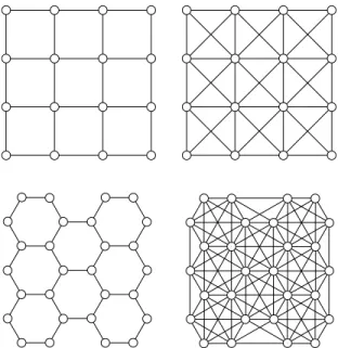
Monotonicity and continuity properties of the function rcG(p) for general graphs have been studied inB´alint et al.(2013). Here we will focus on two specific graphs, namely the square latticeZ2and the hexagonal lattice H (see Figure1.1), for which pZc2 = 1/2 and pHc = 1− 2 sin(π/18) ≈ 0.6527 (see Kesten(1982)). Our reason for
this restriction is twofold: first, these two are the most commonly considered planar lattices (apart from the triangular lattice T, for which the critical value function rTc has been completely characterized inB´alint et al.(2009)), whence results about these cases are of the greatest interest. On the other hand, the DaC model on these lattices enjoys a form of duality (described in Section2.2) which is a key ingredient for the analysis we perform in this paper.
Figure 1.1. A finite sublattice of the square lattice Z2 (above left) and the hexagonal latticeH (below left) and their respective matching lattices (right).
FixingL ∈ {Z2,H}, it is trivial that rL
c (p) = 0 for all p > pLc, and it easily follows
from classical results on Bernoulli bond percolation that rLc(pLc) = 1 (see B´alint et al.(2009) for the caseL = Z2). However, there are only very loose theoretical
bounds for the critical value when p < pLc: the duality relation (2.2) in Section2.2
below and renormalization arguments as in the proof of Theorem 2.6 inH¨aggstr¨om
(2001) give that 1/2≤ rcL(p) < 1 for all such p, and Proposition 1 inB´alint et al.
(2013) gives just a slight improvement of these bounds for very small values of p. Therefore, our ultimate goal here is to get good estimates for rcL(p) with p < pLc.
We end this section with an outline of the paper. Section 2 contains a crucial reduction of the infinite-volume models to a finite situation by a criterion that is
stated in terms of a finite sublattice but nonetheless implies the existence of an infinite cluster. This method, often called static renormalization in percolation, is a particular instance of coarse graining. We then describe in Section 3 how the occurrence of this finite size criterion can be tested in an efficient way and obtain confidence intervals for rcL(p) as functions of uniform random variables (Proposition
3.1). Finally, we implement this method using a (pseudo)random number generator, and present and discuss the numerical results in Section4.
2. Finite size criteria
2.1. An upper bound for rc(p). In this section, we will show how to obtain an upper
bound for rLc(p) by deducing a finite size criterion for percolation in the DaC model (Proposition 2.3). This criterion, which is a quantitative form of Lemma 2.10 in
B´alint et al. (2009), will play a key role in Sections3–4. To enhance readability, we will henceforth focus on the case L = Z2 and mention L = H only when the analogy is not straightforward. Accordingly, we will write Pp,r and rc(p) for PZ
2
p,r
and rcZ2(p) respectively, and denote the edge set ofZ2 by E2. Let us first recall a
classical result (Lemma2.2below) concerning 1-dependent percolation.
Definition 2.1. Given a graph G = (V, E), a probability measure ν on {0, 1}E is called 1-dependent if, whenever S⊂ E and T ⊂ E are vertex-disjoint edge sets, the state of edges in S is independent of that of edges in T under ν.
It follows from standard arguments or from a general theorem of Liggett, Schon-mann and Stacey (Liggett et al.(1997)) that if each edge is open with a sufficiently high probability in a 1-dependent bond percolation on Z2, then the origin is with positive probability in an infinite bond cluster. Currently the best bound is given by Balister, Bollob´as and Walters:
Lemma 2.2. (Balister et al. (2005)) Let ν be any 1-dependent bond percolation measure onZ2in which each edge is open with probability at least 0.8639. Then the
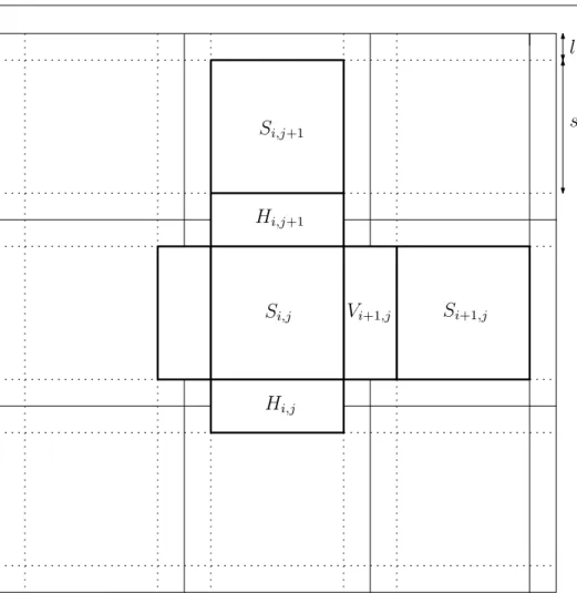
probability under ν that the origin lies in an infinite bond cluster is positive. Now, suppose that the lattice Z2 is embedded in the plane the natural way (so that v = (i, j)∈ Z2 has coordinates i and j). We consider the following partition of R2 (see Figure 2.2): given parameters s ∈ N = {1, 2, . . .} and ` ∈ N, we take k = s + 2` and define, for all i, j∈ Z, the s × s squares
Si,j= [ik + `, ik + ` + s]× [jk + `, jk + ` + s],
the s× 2` rectangles
Hi,j= [ik + `, ik + ` + s]× [jk − `, jk + `],
the 2`× s rectangles
Vi,j= [ik− `, ik + `] × [jk + `, jk + ` + s],
and what remains are the 2`× 2` squares [ik − `, ik + `] × [jk − `, jk + `].
We will couple Pp,r to a 1-dependent bond percolation measure. Define f :
ΩE2× ΩZ2 → ΩE2, as follows. To each horizontal edge e =h(i, j), (i + 1, j)i ∈ E2,
we associate a (2` + 2s)× s rectangle Re = Si,j∪ Vi+1,j ∪ Si+1,j and the event
Ee that there exists a left-right black crossing in Re (i.e., a connected path of
l
s
S
i,jS
i,j+1V
i+1,jS
i+1,jH
i,j+1H
i,j Figure 2.2. A partition of R2.l
s
R
e
Figure 2.3. A black component in Rewitnesses the occurrence of Ee.
corner of a rectangle is understood to link the corresponding sides in itself. For each vertical edge e =h(i, j), (i, j + 1)i ∈ E2, we define the s× (2` + 2s) rectangle
Re= Si,j∪ Hi,j+1∪ Si,j+1 and the event Ee={up-down black crossing in Reand
left-right black crossing in Si,j} ⊂ ΩE2×ΩZ2. For each edge e∈ E2, we also consider
the event Fe ={there exists a bond cluster which contains a vertex in Re and a
vertex at graph distance at least ` from Re} ⊂ ΩE2×ΩZ2, and define ˜Ee= Ee∩Fec.
Now for each configuration ω = (η, ξ)∈ ΩE2× ΩZ2, we determine a corresponding
bond configuration f (ω) = γ∈ ΩE2 as follows: for all e∈ E2, we declare e open if
and only if ˜Ee holds (i.e., we define γ(e) = 1 if and only if ω ∈ ˜Ee). Finally, we
define the probability measure ν = f∗Pp,r on ΩE2.
It is not difficult to check that ν is a 1-dependent bond percolation measure. Indeed, if e and e0 are two vertex-disjoint edges in E2, then the corresponding rectangles Reand Re0 are at graph distance at least 2` from one another, hence Fec
and Fc
e0 are independent. Given that Fe and Fe0 do not hold, the bond clusters in
Re and Re0 are colored independently of each other. Keeping this in mind, a short
computation proves the independence of ˜Eeand ˜Ee0 underPp,r, which implies the
1-dependence of ν.
Note also that the function f was chosen in such a way that if γ = f (ω)∈ ΩE2
contains an infinite open bond cluster, then ω contains an infinite black clus-ter. Such configurations have zeroPp,r-measure for r < rc(p). Finally, note that
Pp,r( ˜Ee) is the same for all edges e∈ E2. These observations combined with Lemma
2.2imply that, denotingh(0, 0), (0, 1)i ∈ E2 by e1, we have the following result.
Proposition 2.3. Given any values of the parameters s, `∈ N, if p and r are such
that
Pp,r( ˜Ee1)≥ 0.8639, (2.1)
then rc(p)≤ r.
Note that Proposition 2.3 is indeed a finite size criterion since the event ˜Ee1
depends on the state of a finite number of edges and the color of a finite number of vertices. A similar criterion, which will imply a lower bound for rc(p), will be
given in Section2.3.
2.2. Duality. A concept that is essential in understanding site percolation models onL ∈ {Z2,H} is that of the matching lattice L∗ which is a graph with the same
vertex set,V, as L but more edges: the edge set E∗ ofL∗ consists of all the edges in E plus the diagonals of all the faces of L (see Figure 1.1). The finiteness of a monochromatic cluster inL can be rephrased in terms of circuits of the opposite color inL∗and vice versa; seeKesten(1982) for further details. We say that B⊂ V is a black ∗-component in a color configuration ξ ∈ ΩV if it is a black component in terms of the latticeL∗ (i.e., ξ(v) = 1 for all v∈ B and B is connected via E∗).
Accordingly, there is yet another phase transition in the DaC model on L at the point where an infinite black ∗-component appears; formally, for each fixed p∈ [0, 1], one can define r∗c(p,L) as the value such that PLp,r(there exists an infinite black∗-component) is 0 for r < rc∗(p,L) and positive for r > r∗c(p,L). It was proved in B´alint et al.(2009) that there is an intimate connection between all the critical values in the DaC model that we mentioned so far; namely, for all p < pLc,
Actually, this relation was proved only for L = Z2, but essentially the same proof
gives the result for L = H as well. The importance of this result here is that due to the duality relation (2.2), a lower bound for rLc(p) may be obtained by giving an upper bound for r∗c(p,L).
2.3. A lower bound for rc(p). As in Section 2.1, we will focus on L = Z2 since
the caseL = H is analogous; we denote r∗c(p,Z2) here and in the next section by
r∗c(p). Obviously rc(p) itself is an upper bound for rc∗(p). However, a better bound
may be obtained by a slight modification of the approach given in Section2.1. For each e∈ E2, let R
e and Fe be as in Section 2.1, define Ee∗ by substituting black
∗-component for black component in the definition of Ee, and take ˜Ee∗= Ee∗∩ Fec.
Then, by similar arguments as those before Proposition2.3and using (2.2), we get the following:
Proposition 2.4. Given any values of the parameters s, `∈ N, if p and r are such
that
Pp,r( ˜Ee∗1)≥ 0.8639, (2.3)
then r∗c(p)≤ r, and hence rc(p)≥ 1 − r.
3. The confidence interval
The main idea inBalister et al.(2005);Riordan and Walters(2007) is to reduce a stochastic model to a new model in finite volume by criteria similar in spirit to those in Section 2 and do repeated (computer) simulations of the new model to test whether the corresponding criteria hold. The point is that after a sufficiently large number of simulations, one can see with an arbitrarily high level of confidence whether or not the probability of an event exceeds a certain threshold. By the special nature of the events in question, statistical inferences regarding the original, infinite-volume model may be made from the simulation results.
To be able to follow this strategy, we will have to refine Propositions2.3–2.4 as those are concerned with the state of finitely many objects, but still in the infinite-volume model. The adjusted criteria that truly are of finite size are given below, see (3.1) and (3.2). Finding an efficient way of performing the simulation step involves further obstacles. The main problem is that it would be unfeasible to run a large number of separate simulations for different values of r to find, for a fixed p, the lowest value of r such that both (3.1) and (3.2) seem sufficiently likely to hold. We will tackle this difficulty with a stochastic coupling, which is the simultaneous construction of several stochastic models on the same probability space. Such a construction will enable us to deal with all values of r∈ [0, 1] at the same time and is very related to the model of invasion percolation.
After the description of the coupling, a “theoretical” confidence interval (meaning a confidence interval as a function of i.i.d. random variables) for rc(p) is given in
Proposition3.1. The numerical confidence intervals obtained by this method using computer simulations will be presented in Section4. Note also that the inequalities (3.1) and (3.2) implicitly involve the parameters s and ` whose choices may influence the width of the confidence intervals obtained; this issue is addressed before the proof of Proposition3.1. Our methods in this section work for a general p∈ [0, pLc); we note that substantial simplifications are possible in the case p = 0 (i.e., in the absence of correlations), seeRiordan and Walters(2007).
Fix p∈ [0, 1/2) and s, ` ∈ N, and define the rectangle ˜Re1= [0, 2s+4`]×[0, s+2`].
Note that for a configuration ω ∈ ΩE2× ΩZ2, one can decide whether ω ∈ ˜Ee1
(respectively ω∈ ˜Ee∗1) holds by checking the restriction of ω to ˜Re1. In fact, defining
˜
G = (˜V, ˜E) as the minimal subgraph of Z2 which contains ˜R
e1 and considering the
DaC model on ˜G, it is easy to see that for any r∈ [0, 1], PG˜
p,r( ˜Ee1) =Pp,r( ˜Ee1) and
PG˜
p,r( ˜Ee∗1) =Pp,r( ˜E
∗
e1). (These equalities hold despite the fact thatP
˜
G
p,r is not the
same distribution as the projection of Pp,r on ˜G.) Therefore, by Propositions 2.3
and2.4,
PG˜
p,r( ˜Ee1)≥ 0.8639 (3.1)
would imply that rc(p)≤ r, and
PG˜
p,r( ˜Ee∗1)≥ 0.8639 (3.2)
would imply that rc(p) ≥ 1 − r. Below we shall describe a method which tests
whether (3.1) or (3.2) holds, simultaneously for all values of r∈ [0, 1].
We construct the DaC model on ˜G with parameters p and an arbitrary r∈ [0, 1] as follows. Fix an arbitrary deterministic enumeration v1, v2, . . . , v|˜V|of the vertex
set ˜V, and for V ⊂ ˜V, let min(V ) denote the vertex in V of the smallest index. For all r∈ [0, 1], we define the function
Ψr : ΩE˜× [0, 1] ˜ V → Ω˜ E× ΩV˜, (η, U ) 7→ (η, ξr), where ξr(v) = { 1 if U (min(Cv(η))) < r, 0 if U (min(Cv(η)))≥ r.
Now, ifU denotes uniform distribution on the interval [0, 1] and (η, U) ∈ ΩE˜×[0, 1] ˜ V
is a random configuration with distribution νpE˜⊗ UV˜, then it is not difficult to see that (η, ξr) = Ψr((η, U )) is a random configuration with distributionP
˜
G p,r.
We are interested in the following question: for what values of r does (η, ξr)∈ ˜Ee1
(respectively, (η, ξr) ∈ ˜E∗e1) hold? The first step is to look at the edges in η in
˜
Re1\ Re1 to see if there is a bond cluster which connects Re1 and the boundary of
˜
Re1. If no such connection is found, it is easy to see that there exists a threshold
value r1 = r1(η, U ) ∈ [0, 1] such that for all r ∈ [0, r1), (η, ξr) /∈ ˜Ee1, and for all
r∈ (r1, 1], we have that (η, ξr)∈ ˜Ee1. Indeed, the color configurations are coupled
in such a way that if r0 ≥ r and (η, ξr)∈ ˜Ee1 then (η, ξr0)∈ ˜Ee1, since all vertices
that are black in ξr are black in ξr0 as well. A similar argument shows that in
case of η /∈ Fe1, there exists r1∗ = r∗1(η, U ) ∈ [0, 1] such that (η, ξr) /∈ ˜Ee∗1 for all
r ∈ [0, r∗1), whereas (η, ξr) ∈ ˜E∗e1 for all r ∈ (r
∗
1, 1]. Otherwise, i.e., if there is a
connection in η between Re1 and the boundary of ˜Re1, we know that neither of ˜Ee1
or ˜Ee∗
1 has occurred. Hence, in that case, we define r1= r
∗
1 = 1, which preserves
the above “threshold value” properties as (r1, 1] = (r∗1, 1] =∅.
Now, if we want a confidence interval with confidence level 1− ε where ε > 0 is fixed, we choose positive integers m and n in such a way that the probability of having at least m successes among n Bernoulli experiments with success proba-bility 0.8639 each is smaller than (but close to) ε/2. For instance, for a 99.9999% confidence interval, we can choose n = 400 and m = 373. By repeating the above experiment n times, each time with random variables that are independent of all
the previously used ones, we obtain threshold values r1, r2, . . . , rnand r∗1, r2∗, . . . , r∗n.
Then we sort them so that ˜r1≤ ˜r2≤ ... ≤ ˜rn, and ˜r∗1≤ ˜r∗2≤ ... ≤ ˜rn∗.
Proposition 3.1. Each of the inequalities rc(p)≤ ˜rm and 1− ˜rm∗ ≤ rc(p) occurs
with probability at least 1− ε/2, hence [1 − ˜rm∗, ˜rm] is a confidence interval for rc(p)
of confidence level 1− ε.
Before turning to the proof, we remark that the above confidence interval does not necessarily provide meaningful information. In fact, with very small (< ε) probability, ˜rm< 1− ˜rm∗ can occur. Otherwise, for unreasonable choices of s and
`, taking a too small ` in particular, it could happen that there is a connection in the bond configuration between Re1 and the boundary of ˜Re1 in at least n− m + 1
experiments out of the n, in which case [1− ˜r∗m, ˜rm] = [0, 1] indeed contains rc(p)
but gives no new information.
However, the real difficulty is that although a confidence interval with an arbi-trarily high confidence level may be obtained with the above algorithm, we do not know in advance how wide the confidence interval is. The width of the interval depends on s and `, and it is a difficult problem to find good parameter values. A way to make the confidence interval narrower is to decrease the value of m, but that comes at the price of having a lower confidence level.
The choices we made for the parameters s and ` in our simulations, together with some intuitive reasoning advocating these choices, are given in the Appendix.
Proof of Proposition3.1. LetS be the probability measure on the sample space
[0, 1]2n which corresponds to the above experiment, where a realization
(˜r1, ˜r∗1, ˜r2, ˜r2∗, . . . , ˜rn, ˜rn∗) contains the (already ordered) threshold values. LetB0.8639
denote the binomial distribution with parameters n and 0.8639, andBa(r) the
bi-nomial distribution with parameters n and a(r) =PG˜ p,r( ˜Ee1).
For r ∈ [0, 1], let Nr denote the number of trials among the n such that ˜Ee1
occurs at level r. Note that Nr has distributionBa(r). Since a(r)≥ 0.8639 implies
r ≥ rc(p) (see inequality (3.1)), we have that r < rc(p) implies a(r) < 0.8639.
Therefore, for all r < rc(p), Ba(r) is stochastically dominated by B0.8639. This
implies that for all r < rc(p), we have that
S(˜rm< r) ≤ S(Nr≥ m)
= Ba(r)({m, m + 1, . . . , n})
≤ B0.8639({m, m + 1, . . . , n})
≤ ε/2, by the definition of m and n.
Hence, for all δ > 0, we have thatS(˜rm< rc(p)− δ) ≤ ε/2, which easily implies
that S(˜rm < rc(p)) ≤ ε/2. We also have S(˜rm∗ < r∗c(p)) ≤ ε/2 by a completely
analogous computation, which implies by equation (2.2) thatS(1 − ˜rm∗ > rc(p))≤
ε/2. Therefore,
S(1 − ˜r∗
m≤ rc(p)≤ ˜rm)≥ 1 − ε,
4. Results of the simulations
We implemented the method described in the previous section in a computer program, and the results for parameter values ε = 10−6, n = 400, m = 373 are given below.1 We stress again that although the method in Section 3 that determines a confidence interval for rcL(p) is mathematically rigorous, the results below are obtained by using the random number generator (Mersenne Twister, available at
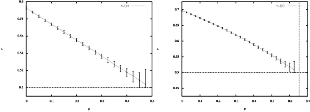
http://www.math.sci.hiroshima-u.ac.jp/), therefore their correctness depends on “how random” the generated numbers are. The simulations ran on the computers of the ENS-Lyon, and yielded the confidence intervals represented in Figure4.4.
0.5 0.52 0.54 0.56 0.58 0.6 0 0.1 0.2 0.3 0.4 0.5 r p 0.5 0.52 0.54 0.56 0.58 0.6 0 0.1 0.2 0.3 0.4 0.5 r p 0.5 0.52 0.54 0.56 0.58 0.6 0 0.1 0.2 0.3 0.4 0.5 r p 0.5 0.52 0.54 0.56 0.58 0.6 0 0.1 0.2 0.3 0.4 0.5 r p rc(p) 0.45 0.5 0.55 0.6 0.65 0.7 0 0.1 0.2 0.3 0.4 0.5 0.6 0.7 r p 0.45 0.5 0.55 0.6 0.65 0.7 0 0.1 0.2 0.3 0.4 0.5 0.6 0.7 r p 0.45 0.5 0.55 0.6 0.65 0.7 0 0.1 0.2 0.3 0.4 0.5 0.6 0.7 r p 0.45 0.5 0.55 0.6 0.65 0.7 0 0.1 0.2 0.3 0.4 0.5 0.6 0.7 r p rc(p)
Figure 4.4. Simulation results for different values of p < pLc (left:
on the square lattice; right: on the hexagonal lattice). The dashed line was obtained via a non-rigorous correction method.
Having looked at Figure4.4, we conjecture the following concerning the behavior of rLc(p) as a function of p:
Conjecture 4.1. For L ∈ {Z2,H}, in the interval p ∈ [0, pL
c), rLc(p) is a strictly
decreasing function of p and
lim
p→pLc−
rcL(p) = 1 2.
Since it is rigorously known that rLc(0) > 1/2 and rLc(p)≥ 1/2 for all p ∈ [0, pLc), Conjecture 4.1 would imply that rcL(p) > 1/2 for all p < pLc. This suggests that the DaC model on Z2 or H is qualitatively different from the DaC model on the
triangular lattice, where the critical value of r is 1/2 for all subcritical p (see Theorem 1.6 inB´alint et al. (2009)). However, lim rLc(p) = 1/2 would mean that the difference disappears as p converges to pLc.
The fact that the difference should disappear was conjectured by one of the authors (VB) and Federico Camia, based on the following heuristic reasoning. Near p = pLc, the structure of the random graph determined by the bond configuration (whose vertices correspond to the bond clusters, and there is an edge between two vertices if the corresponding bond clusters are adjacent inL) is given by the geometry of “near-critical percolation clusters,” which is expected to be universal for 2-dimensional planar graphs. This suggests that the critical r for p close to its
1These results — without the description of the method — have been included inB´alint et al. (2013) as well.
critical value should not depend much on the original underlying lattice, and we expect the convergence of rcL(p) to 1/2 to be universal and hold in the case of any 2-dimensional lattice.
There is an additional, strange feature appearing in the case of the square lattice: rc(p) seems to be close to being an affine function of p on the interval [0, 1/2).
This is not at all the same on the hexagonal lattice, and we have not found any interpretation of this observation, or of the special roleZ2seems to play here.
Open question 4.2. Is rZc2(p) an affine function of p for p < 1/2?
Acknowledgments. We thank Federico Camia and Ronald Meester for interesting
and useful discussions and valuable comments on an earlier version of this paper. V.T. thanks for the hospitality of the VU University Amsterdam where much of the work reported here was derived during an internship provided by ENS Lyon.
Appendix A.
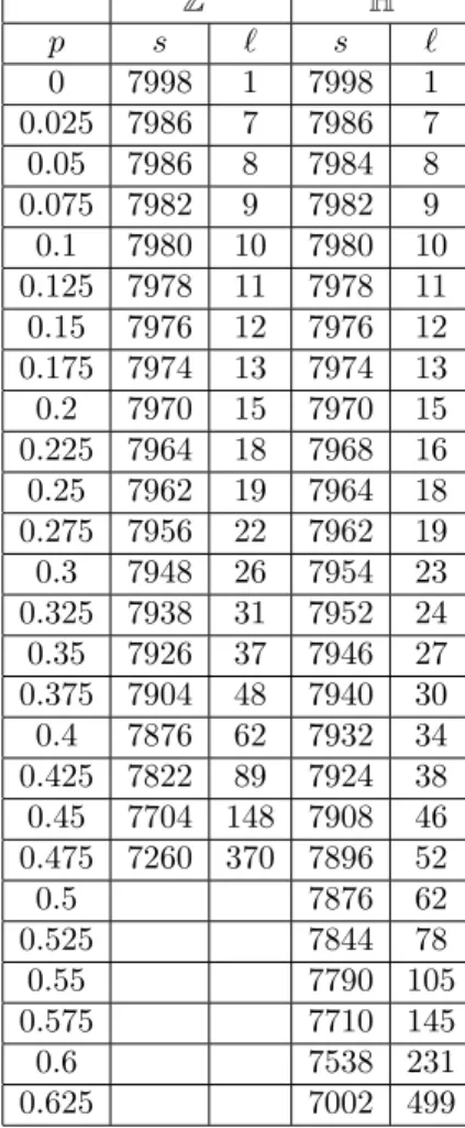
The algorithm in Section 3 is described for general values of s and `, and the concrete values of these parameters will not affect the correctness of the simulation results. However, a reasonable choice is important for the tightness of the bounds obtained and the efficiency of the algorithm, i.e., the running time of the program. The heuristic arguments given here are somewhat arbitrary, and it is quite possible that there exist other choices that would give at least as good results as ours.
Applying the method described in Section3requires to simulate a realization of the DaC model on the graph ˜G, which is a 2L× L rectangular subset of the square lattice where
L = s + 2`. (A.1)
We will keep this value fixed while we let ` and s depend on p. Since we want to estimate the critical value for a phase transition, it is natural to take the largest L possible. After having performed various trials of our program, we chose L = 8000, which was estimated to be the largest value giving a reasonable time of computation. Having fixed the size of the graph, we want to choose the parameters so that the probability of ˜Ee1 is as high as possible. We need to find a balanced value
for ` as small values favor Ee1, but a large ` might be required to prevent Fe1
from happening. The exponential decay theorem inAizenman and Barsky(1987);
Menshikov(1986) for subcritical Bernoulli bond percolation ensures the existence of an appropriate ` of moderate size. In our context, we decided that a good ` = `(p) would be one that ensures
PG˜
p,r(Fe1)≈ 0.001. (A.2)
We did simulations in order to find an ` such that (A.2) holds, then chose s ac-cording to equation (A.1). The values we used in our simulations are summed up in TableA.1.
Z2 H p s ` s ` 0 7998 1 7998 1 0.025 7986 7 7986 7 0.05 7986 8 7984 8 0.075 7982 9 7982 9 0.1 7980 10 7980 10 0.125 7978 11 7978 11 0.15 7976 12 7976 12 0.175 7974 13 7974 13 0.2 7970 15 7970 15 0.225 7964 18 7968 16 0.25 7962 19 7964 18 0.275 7956 22 7962 19 0.3 7948 26 7954 23 0.325 7938 31 7952 24 0.35 7926 37 7946 27 0.375 7904 48 7940 30 0.4 7876 62 7932 34 0.425 7822 89 7924 38 0.45 7704 148 7908 46 0.475 7260 370 7896 52 0.5 7876 62 0.525 7844 78 0.55 7790 105 0.575 7710 145 0.6 7538 231 0.625 7002 499
References
M. Aizenman and D. J. Barsky. Sharpness of the phase transition in percolation models. Comm. Math. Phys. 108 (3), 489–526 (1987). MR874906.
A. B´alint, V. Beffara and V. Tassion. On the critical value function in the divide and color model. ALEA 10, 653–666 (2013).
A. B´alint, F. Camia and R. Meester. Sharp phase transition and critical behaviour in 2D divide and colour models. Stochastic Process. Appl. 119 (3), 937–965 (2009). MR2499865.
P. Balister, B. Bollob´as and M. Walters. Continuum percolation with steps in the square or the disc. Random Structures Algorithms 26 (4), 392–403 (2005).
MR2139873.
L. Chayes, J. L. Lebowitz and V. Marinov. Percolation phenomena in low and high density systems. J. Stat. Phys. 129 (3), 567–585 (2007). MR2351418.
M. Deijfen, A. E. Holroyd and Y. Peres. Stable Poisson graphs in one dimension. Electron. J. Probab. 16, no. 44, 1238–1253 (2011). MR2827457.
B. Graham and G. Grimmett. Sharp thresholds for the random-cluster and Ising models. Ann. Appl. Probab. 21 (1), 240–265 (2011). MR2759201.
J. Gravner, D. Pitman and S. Gavrilets. Percolation on fitness landscapes: effects of correlation, phenotype, and incompatibilities. J. Theoret. Biol. 248 (4), 627–645 (2007). MR2899086.
O. H¨aggstr¨om. Coloring percolation clusters at random. Stochastic Process. Appl.
96 (2), 213–242 (2001). MR1865356.
C. Hsu and D. Han. Asymptotic behavior of percolation clusters with uncorrelated weights. Theoret. and Math. Phys. 157 (2), 309–320 (2008). MR2493783. H. Kesten. Percolation theory for mathematicians, volume 2 of Progress in
Prob-ability and Statistics. Birkh¨auser Boston, Mass. (1982). ISBN 3-7643-3107-0.
MR692943.
T. M. Liggett, R. H. Schonmann and A. M. Stacey. Domination by product mea-sures. Ann. Probab. 25 (1), 71–95 (1997). MR1428500.
M. V. Menshikov. Coincidence of critical points in percolation problems. Dokl. Akad. Nauk SSSR 288 (6), 1308–1311 (1986). MR852458.
O. Riordan and M. Walters. Rigorous confidence intervals for critical probabilities. Phys. Rev. E 76, 011110 (2007). DOI: 10.1103/PhysRevE.76.011110.