Precise and modular static analysis by abstract interpretation for the automatic proof of program soundness and contracts inference

(1)

HAL Id: tel-02947214

https://tel.archives-ouvertes.fr/tel-02947214

Submitted on 23 Sep 2020

HAL is a multi-disciplinary open access archive for the deposit and dissemination of sci-entific research documents, whether they are pub-lished or not. The documents may come from teaching and research institutions in France or abroad, or from public or private research centers.

L’archive ouverte pluridisciplinaire HAL, est destinée au dépôt et à la diffusion de documents scientifiques de niveau recherche, publiés ou non, émanant des établissements d’enseignement et de recherche français ou étrangers, des laboratoires publics ou privés.

Precise and modular static analysis by abstract

interpretation for the automatic proof of program

soundness and contracts inference

Matthieu Journault

To cite this version:

Matthieu Journault. Precise and modular static analysis by abstract interpretation for the automatic proof of program soundness and contracts inference. Programming Languages [cs.PL]. Sorbonne Université, 2019. English. �NNT : 2019SORUS152�. �tel-02947214�

(2)

THÈSE DE DOCTORAT DE SORBONNE UNIVERSITÉ

Spécialité Informatique

École doctorale Informatique, Télécommunications et Électronique (Paris) Présentée par

Matthieu Journault

Pour obtenir le grade de

DOCTEUR de SORBONNE UNIVERSITÉ

Sujet de la thèse :

Analyse statique modulaire précise par interprétation abstraite pour

la preuve automatique de correction de programmes et pour

l’inférence de contrats.

soutenue le 21 Novembre 2019 devant le jury composé de :

M. Antoine MINé Directeur de thèse Mme. Sandrine BLAZY Rapporteure

M. Andy KING Rapporteur

M. Emmanuel CHAILLOUX Examinateur M. Tristan LE GALL Examinateur M. Pascal SOTIN Examinateur

(3)

(4)

i

Résumé

Assurer le passage à l’échelle des analyseurs statiques définis par interprétation abstraite pose des difficultés à la fois techniques et pratiques. Une méthode classique d’accélération consiste en la découverte et la réutilisation de contrats satisfaits par certaines comman-des du code source (par exemple, le corps d’une fonction). Cette thèse s’intéresse à un sous-ensemble de C qui ne permet pas la récursivité, pour lequel on définit un analyseur modulaire capable d’inférer, de prouver et d’exploiter de tels contrats. Ces contrats sont: (1) précis: ils permettent d’exprimer une relationnalité numérique entre les états d’entrée et de sortie à travers l’utilisation de domaines numérique relationnels; (2) corrects: utiliser un contrat précédemment inféré pour une commande produit un état de sortie surapproxi-mant l’ensemble des états effectivement atteignables à la fin de ladite commande; (3) dirigés par les entrées: des contrats ne sont découverts que pour les contextes d’appel rencontrés pendant l’analyse; si une divergence apparait, un opérateur d’élargissement est utilisé pour stabiliser les contextes d’entrée. Notre analyseur modulaire est défini au dessus d’un anal-yseur C existant et est donc capable de manipuler des types unions, des types structures, des tableaux, des allocations de mémoire (statique et dynamique), des pointeurs, y compris l’arithmétique de pointeur et le transtypage, appels de fonction, des chaînes de caractères, .... La représentation des chaînes de caractère est gérée par un nouveau domaine abstrait défini dans cette thèse. Ce domaine abstrait de chaînes stocke avec précision la longueur des chaînes C (position du premier '\0') sans recourir à une représentation explicite des tableaux, qui peut devenir coûteuse, ce qui est utile pour prouver l’absence d’accès hors mémoire lors de manipulations de chaîne.

La plupart des domaines abstraits numériques utilisés dans le cadre de l’interprétation ab-straite se concentrent sur la représentation d’ensembles de fonctions numériques partageant le même ensemble de définition. Si des ensembles hétérogènes apparaissent pendant une analyse, la plupart des analyseurs ont recours à du partitionnement ou à des méthodes non relationnelles. Dans cette thèse, nous proposons une technique paramétrique de transfor-mation de la sémantique classique des domaines abstraits vers une sémantique d’ensembles hétérogènes. Cette technique peut être utilisée pour des domaines relationnels et ne main-tient qu’un seul état abstrait numérique, par opposition au partitionnement. De plus, lorsque l’ensemble est homogène, on retrouve la précision et la complexité des domaines classiques. Le dernier point d’intérêt de cette thèse est la définition d’un domaine abstrait capa-ble de représenter des ensemcapa-bles d’arbres dont les feuilles peuvent contenir des labels numériques. Cette abstraction est basée sur les langages régulier et les langages d’arbre régulier, et délègue une partie de son abstraction à un domaine numérique sous-jacent capa-ble de représenter des ensemcapa-bles d’environnements hétérogènes. Cette abstraction d’arbres a plusieurs applications parmi lesquelles: la représentation de la mémoire pour les langages fournissant des structures arborescentes, le développement d’un domaine sauvegardant des égalités symboliques entre les variables et les expressions dans un programme, le développe-ment d’une pré-analyse pour le language C, fournissant des informations de framing.

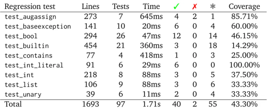
Cette thèse s’étant déroulée dans le projet MOPSA, nous donnons un aperçu de certains ré-sultats obtenus par l’équipe pendant la thèse. De plus, tous les domaines abstraits présentés ici ont été implantés dans l’analyseur statique MOPSA, une discussion sur certains résultats expérimentaux préliminaires est fournie pour chaque domaine.

(5)

ii

Abstract

Ensuring the scalability of static analyzers defined by abstract interpretation poses both theoretical and practical difficulties. A classical technique known to speed up analyses is the discovery and reuse of summaries for some of the sequences of statements of the source code (e.g. functions bodies). In this thesis we focus on a subset of C that does not allow recursion and define a modular analyzer, able to infer, prove and use (to improve the efficiency) such summaries. The summaries considered here are (1) precise: they allow input/output numer-ical relationality via the use of relational numernumer-ical domain; (2) sound: the use of a summary inferred for a statement represents an over-approximation of the reachable set of states at the end of the considered statement; (3) inputs oriented: summaries are inferred only for calling contexts met during the analysis, if a divergence occurs a widening operator is used to stabilize input contexts. Our modular analyzer is built on top of a existing C analyzer and is therefore able to handle unions, structures, arrays, memory allocations (static and dynamic), pointers, pointer arithmetics, pointer casts, function calls, string manipulations,…. String handling is provided by a new abstract domain defined in this thesis, this string abstract domain aims at precisely tracking the length of C strings (position of the first'\0'), which is helpful to prove the absence of out-of-memory accesses in string manipulations.

Most numerical abstract domains used in the abstract interpretation framework focus on the representation of sets of numerical maps that all share the same definition set. When the need arises to represent heterogeneous sets of maps, most analyzers fall back to the use of partitioning. In this thesis we provide a lifting of classically used abstract domains to the representation of heterogeneous sets. This lifting can be used for relational domains and maintains only one numerical abstract state, by opposition to partitioning. Moreover when the set is homogeneous the lifted domain behaves as the underlying numerical domain in terms of both precision and efficiency.

The last point of interest of this thesis is the definition of an abstract domain able to rep-resent sets of trees with numerically labeled leaves. This abstraction is based on regular and tree regular languages and delegates the handling of numerical constraints to an underly-ing domain able to represent heterogeneous sets of environments. This tree abstraction has several applications among which: memory representation for languages providing tree-like structures, the development of a domain tracking symbolic equalities between variables and expressions in a program, the development of a pre-analyzer providing framing information for the C language.

As the thesis took place in the MOPSA project, we provide an overview of some of the results obtained by the MOPSA team during the thesis. Finally, all domains presented in the thesis have been implemented as abstract domains in the MOPSA static analyzer, therefore some preliminary experimental results are presented and discussed in the thesis.

(6)

Introduction

The increasing usage of software in various fields (aeronautic industry, medical world, army, …) is an area of concern as we have witnessed in the past years several failures of such soft-ware. As examples, let us mention the Ariane 5 failure (caused by an integer overflow and an unhandled exception) [Le 97], the Patriot missile battery at Dhahran [Ske92], and finally the infamous Therac-25 radiation therapy machine which administered excessive quantities of beta radiation [LT93].

In order to prevent these from happening, we first need to detect that such failures may occur. Two approaches can be taken in catching these failures. The first method is to add dynamic testing, meaning that while the software is running it self-checks its behavior, in case of an error the execution is stopped, potentially leading to other failures. The second method is to discover before the execution of the program whether bugs will occur or not. This can be achieved by testing the program before its deployment, by reviewing the code or finally by using formal methods to obtain mathematical results about the behavior of the program. Among formal methods we can cite: program proving, model-checking and static analysis, all of which are described in the following. A particular attention will be given to static analysis as this is the context of this thesis.

Such failures are moreover very hard to discover by hand and it is even harder to prove the absence of such “bugs” without automation, due to the size of real life software and to the fact that the configuration space might be unbounded. In the process of automating this discovery, one is faced with the theoretical limit that: there exists no programs, taking programs as input and deciding whether or not they terminate [Tur37]. This result is extended by Rice’s theo-rem [Ric53] that states that all non-trivial properties about the language recognized by a Turing machine are undecidable. The set of all possible executions of a software is called its seman-tics and is defined by the programming language. The problem of proving the absence of bugs requires to infer and prove that the semantics of the program satisfies some properties, which can be seen as proving that the semantics of the targeted program is included into the set of all executions satisfying this property. The results above ensure that semantics are not computable in general, moreover they might not be representable in a computer.

As for other fields of computer science, a notion of soundness and completeness are defined. We say that a static analysis is sound with respect to the concrete semantics when the set of program executions considered by the analysis is greater than the actual semantics, conversely we say that it is complete when it is lower. As we have seen, a sound, complete and automatic analyzer able to handle all programs can not be designed. This leaves us with several choices: (1) giving up on Turing complete languages; (2) choosing any two of the three properties (sound, complete, automated) and giving up on the last. These observations led to the creation and development of several fields of computer science, their objective ranging from discovering bugs in software to mathematically proving that all executions of a program behave as its specifications asserts. The work presented in this thesis is automated and sound but is not complete in general.

(11)

2 CHAPTER 1. INTRODUCTION

In the next section we provide a small overview of some of the fields of program verification.

1.1 Program verification

1.1.1 Tests

In most cases, the only static analysis performed on programs is testing. Testing consists in launching the targeted program on some inputs (a finite number) and verifying that the prop-erty holds on this particular execution. Testing can be done by hand, by executing the program on some well-chosen inputs, or automatically by generating inputs (e.g. see [CH00]). This gen-eration can be uniform and/or guided by the program. Note that, for a program failing on only one of its 232possible inputs (imagine for example an integer overflow), uniform testing will find the error with probability 2−32_{. Moreover each input requires a run of the targeted program,}

which may be slow to execute or might not terminate at all. In any cases, if the input space is not bounded, testing is a complete and automated but unsound technique to prove that some property holds on the semantics of a program. Indeed only a finite number of executions can be checked.

1.1.2 Model Checking

Model Checking [CGP99, QS82] is a sound and complete verification process for transition sys-tems that are finite or enjoy more regularity than that provided by Turing complete programming languages. The set of properties that can be checked is restricted to some logic (e.g. CTL, LTL), and the framework provides algorithms that can check whether a given structure is a model of a formula of this logic or not. When starting from a transition system too expressive for model checking, one can sometimes refine it by hand (by removing information useless to proving the targeted property) to its core behavior and perform model checking on the result. A classical introductory example of model checking is the beverage dispenser machine. This machine has several (a finite number) states and changes states according to user inputs, incoming money, beverage being dispensed, …. The property – if I input enough money, I will get a beverage at some point – can be encoded into a temporal logic, a predefined algorithm can thus check whether the description of the beverage dispensing machine satisfies the above property.

1.1.3 Program proving

One can analyze a program by hand by providing and proving properties satisfied by the seman-tics of the program. This can be helped and in some place automated using theorem provers (see for example Coq). This approach may lead to complete and sound reasoning about the semantics of a program, hence statically providing very powerful properties about executions of the program such as: this function adds an element to the tree and yields a balanced tree. Type systems, in a language such as OCaml, are a particular case of program proving restricted to a subset P of properties for which inferring and proving the strongest property satisfied by the program inP is decidable and has a “reasonable” time complexity (an example of property is f: 'a -> 'a, stating thatf always outputs a value of the same type as its input). Program proving has been used successfully in the past years, leading to the development of software that are mathematically proved to follow their specifications (e.g. CompCert [Ler09]). Program proving is very powerful, but demands that programmers write proofs that their programs sat-isfy (potentially complicated) properties. This can be done as a part of the development process for some targeted software, however for existing codes and for most of the software written in industry this does not seem achievable. Deductive verification tools (such as Why3) only asks the user to provide invariants and contracts for loops and functions from the source code. Proof goals for these contracts and invariants are automatically generated, provers (such as Z3) then

(12)

1.2. CONTENT OF THE THESIS 3

try to automatically prove these goals. This offers a less powerful but more automatic approach to theorem proving than theorem provers.

1.1.4 Abstract interpretation

Abstract interpretation [CC77b] is a theory formalizing semantics approximations. As the seman-tics of programs is not computable we build a sequence of semanseman-tics, each being an abstraction of the previous one (the notion of abstract/concrete semantics is relative). The goal of building such sequences is to forget information from the original semantics, the choice of how precision is lost being guided by the targeted properties. The last abstract semantics of the sequence is designed so that: (1) elements of this abstract semantics are machine representable; (2) usual semantics operators (union, transitions in the original system, fixpoint computations) are com-putable. As abstractions might lose information about the original semantics, results discovered on the abstract semantics may not always be exact. The goal of abstract interpretation being to certify software, we want to obtain properties of the form “no integer overflow will occur during the execution of this program”. Therefore the information loss yielding computability results can not be obtained by removing elements from the original semantics, otherwise it would be possible in the abstract worlds to observe the absence of integer overflow without it implying the same in the original world. For this reasons we chose to over-approximate the concrete seman-tics during the approximation steps. As mentioned above, the semanseman-tics S of a program (and more generally of a transition system) is the set of all its possible executions, a property can be defined as the set of all execution that do satisfy this property P. Proving that the semantics satisfy the property, amounts to showing that S⊆ P, it is therefore sufficient to show that a set of states containing S is included in the propertyP.

Abstract interpretation is fully automatic, in the sense that the user designs abstract domains which will be able to precisely represent a (potentially unbounded) subset of all the possible properties. Abstract domains will then be able, given a program, to infer and prove that some property holds on the semantics of this program. As we mentioned, information may be lost due to over-approximations and therefore abstract interpretation provides sound but incomplete analyzers. This induces false positives being potentially reported by the analyzer.

The above mentioned abstract domains enjoy several composition mechanisms that can be used to target different input language features, or even refine each other in order to gain preci-sion. This allows the designers of abstract domains to focus on building high precision analyses for small features of the language, as these will then be composed with already existing abstract domains tackling the rest of the language.

Abstract interpretation has enjoyed a growing success, as witnessed by commercial tools used in the industry: Polyspace Verifier, Astrée [KWN+_{10], Sparrow [OHL}+_{12], Julia [Spo05], etc.}

Astrée was able to prove the absence of run-time errors in real life critical software such as the flight control software of the Airbus A340 fly-by-wire system, a program of 132,000 lines of C. Open-source industrial-strength frameworks to design analyzers by abstract interpretation have also been proposed: Frama-C [CKK+_{12], IKOS [BNSV14], Infer [CDD}+_{15a], etc.}

1.2 Content of the thesis

This thesis was made in the scope of Abstract interpretation. In this section we provide an overview of the different topics addressed in this thesis, as well as the reasons why these topics were chosen. These can be sorted into 5 categories: modularity, strings, numeric, trees, analyzer design and implementation.

Modularity. Modularity is to be understood in the sense that the analysis of a large software can be obtained as a composition of the analysis of the different parts composing the software

(13)

1 int incr(int x) { 2 int y = x+1; 3 return (y); 4 } 5 6 int main() { 7 int a = incr(0); 8 int b = incr(1); 9 … 10 } Program 1.1: Modularity example 1 while (*q != '\0') { 2 *p = *q; 3 p++; 4 q++; 5 } 6 *p = *q;

Program 1.2: C String copy

(this can be applied at different scales: functions, libraries, …). Radhia Cousot and Patrick Cousot mention in [CC02], that performing modular analysis is a way to improve scalability of analyzers defined by abstract interpretation. Indeed as software may contain hundreds of thou-sands lines of codes, the ability to reduce the complete analysis to the composition of analysis results of its different parts may induce a great speed up. Moreover if, during the development, a component is not modified between two versions of the software, the results of its analysis in the first version may be reused for the second one, leading to incremental analyses. In the above presentation, we mentioned that the goal of analyzers defined by abstract interpretation is to compute an over-approximation of the semantics of a program. This over-approximation is obtained by following the definition of the original semantics of the program, by replacing the usual semantics operator (union, transitions, fixpoint computation, …) by an abstract coun-terpart. Consider the small example of Program 1.1, this program contains an incrementation functionincr. The behavior of function maindepends on the behavior of functionincr. A non modular analysis will follow the execution of this program, therefore the body of functionincr will be visited at least twice. However, in a modular analysis, we would start by inferring from the body of functionincrthat: ∀x,incr(x)=x+ 1. This fact describes completely the behavior ofincr, which will therefore not be visited again. When trying to design a modular analysis in the framework of abstract interpretation, one is faced with two challenges: precision and cost. Indeed during a classical analysis of a program, we do not compute an over-approximation of the semantics of all statements appearing in the program, we rather compute an over-approximation of the part of the semantics that is used for the analysis of the complete program. As an example: it is unnecessary to compute the complete semantics of statementy = x + 1in Program 1.1, as we will only be interested in the cases wherex= 0 orx= 1. Computing the complete semantics of this statement might be more costly than computing only parts of it, however discovering such facts is non trivial when trying to analyze functions independently from one another. Further-more as we perform static analysis by abstract interpretation, semantics are over-approximated. Analyzing a component of the program independently from the rest may lead to a result that is strictly less precise than what we would have obtained by partitioning the context and comput-ing a semantics for each case. A modular analyzer is provided in Chapter 5, this chapter also provides a more detailed introduction to the problem of modular analysis as well as a presenta-tion of already existing works. The modular analyzer of Chapter 5 is able to handle most of the C language features (including pointers) as we designed it on top of an existing analysis for the C language [Min06a]. It performs a top-down analysis of the program, following the control flow. When function calls are encountered the analyzer will (1) use a pre-discovered summary, hence

(14)

1.2. CONTENT OF THE THESIS 5

1 typedef struct node

2 {

3 int data;

4 struct node* next; 5 } node;

6

7 node* append(node* head, int data)

8 {

9 if (head==NULL) {

10 return (create(data, NULL));

11 } else {

12 node *cursor=head;

13 while(cursor->next != NULL) 14 cursor=cursor->next;

15 node* new_node=create(data,NULL); 16 cursor->next=new_node;

17 return head;

18 }

19 }

Program 1.3:appendfunction

avoiding an analysis of the function body, or (2) infer a context-dependant summary . Input contexts are however stabilized by use of widening before analysis, this ensures that, ultimately, summaries are stable. Finally in order to improve precision and reusability, input framing will be used.

Strings. In order to show that modularity can be obtained even for analyzers targeting prop-erties that are not purely numerical, we decided to enrich our C analyzer so that is was able to reason about mutable'\0'-terminated strings. Our analysis handles accesses to strings made via C pointer arithmetic manipulations, as an example consider the string copy from Program 1.2. Strings are used in all C software and are often error prone as they may lead to out-of-bound accesses. This new abstract domain is described in Chapter 4.

Trees. The precision and scalability of our modular static analyzer depends greatly upon the quality of its framing. The frame rule from separation logic [Rey02] enables to lift local reason-ing: if a precondition P of a statement is “extended” with some facts, and the added facts do not interfere with the statement, then these facts can be added to the postcondition obtained from P. In order to improve both precision and analysis time we need our analyzer to “frame” its inputs. As an example consider Program 1.3, describing anappendfunction that adds an integer dat the end of a listh. The behavior ofappendis independent from the content of thedatafields of the list. Discovering this fact would allow us to forget the values contained in these fields be-fore the analysis, and allow reusability of the summary independently from the values contained in the list. This can be achieved by providing the analyzer with facts gathered beforehand by a pre-analysis. We decided to use terms of the C language to describe the memory zones that may be used during a function call, for example in the case of theappend function we would say that only{head,∗(head+ 4), . . .} are used by the function. We were therefore faced with the

(15)

problem of analyzing a language manipulating terms containing numerical values. This led to the development of an abstract domain presented in Chapter 7.

Numeric domains. During the development of the tree abstract domain, we needed to be able to manipulate heterogeneous sets of environments. These are sets of environments that are not all defined on the same support. In classical abstract interpretation, concrete environments from the semantics are abstracted using numerical abstract domains. These domains have been widely studied (see Section 2.4 for an overview), and are able to abstract set of environments defined over a given finite set of variables. However when analyzing dynamic languages like python, or when designing high-level predicate abstractions, we need to represent and manipulate hetero-geneous sets of environments. Very few results gave an answer to this problem, some of them being more “folk results” that were not well-defined, widely used and limited to non relational numerical domains. For these reasons we defined a general lifting of numerical abstract domains to be able to represent heterogeneous environments. This lifting and several of its improvements are presented in Chapter 6. Note moreover that the ability to represent heterogeneous environ-ments can also be used, during a modular analysis, to merge input contexts of a function, not necessarily defined on the same variable set.

MOPSA. This thesis took place in the MOPSA project. The goal of this project is to design and develop a modular framework for the development of static analyzers defined by abstract inter-pretation. All implementations from this thesis were made in the MOPSA static analyzer. This served the dual purpose of: (1) easing the development of the new abstract domains as already existing features could be reused; (2) testing and improving the expressiveness of the MOPSA framework.

1.3 Outline of the thesis

The remainder of the thesis is organized as follow:

• Chapter 2 provides some of the theoretical prerequisites of this thesis.

• Chapter 3 details some of the features of the MOPSA static analyzer. This analyzer is an ongoing project being developed by several persons (including myself), this chapter has therefore a dual purpose: (1) it presents some the work performed on this analyzer during this thesis; (2) it shows some of the features of the analyzer in which all subsequent abstract domains and algorithms of this thesis were implemented.

• Chapter 4 presents an abstract domain targeting the discovery of out-of-bounds accesses in C'\0'-terminated strings. The definition of this abstraction requires to introduce the cell abstraction [Min06a], used to represent C memory manipulation in our analyzer. • Chapter 5 presents a modular analyzer. We start by showing how this modular analyzer

handles numerical programs. Moreover, in order to emphasize that our modular analysis can be used for abstract domains that are not purely numerical, we apply the technique on a abstract domain able to handle the full C language.

• Chapter 6 provides numerical abstractions that enable the representation of set of numer-ical maps that do not necessarily share the same support. These abstractions were first devised because they were needed in: the MOPSA framework, the definition of higher level abstractions as the one of Chapter 7.

• Chapter 7 presents an abstraction for sets of trees with leaves that can be labeled with nu-merical values. The goal of this abstraction is to provide a pre-analysis for the C language. This pre-analysis would be used in combination with results from Chapter 5.

• Chapter 8 concludes the thesis, and puts forth some future works.

• Finally, note that results we deemed proof-worthy are annotated as such in the body of the thesis, proofs can then be found in Appendix A.

(16)

1.3. OUTLINE OF THE THESIS 7

Each chapter (except Chapter 2) features: (1) a motivating introduction, (2) a presentation of related works, (3) some implementation considerations and (4) a conclusion

(17)

(18)

Chapter 2

Background – Abstract interpretation

In this chapter we provide the theoretical background of this thesis. We present here the common part of the prerequisites of all subsequent chapters. Every chapter will then provide backgrounds of their own (such sections are marked with “Background” so as to differentiate contributions from state of the art results). As an example, results from automata theory are used in this thesis but will only be introduced in the Background section of Chapter 7.

This thesis will make extensive use of the abstract interpretation framework [CC77b]. For this reason this chapter is devoted to a presentation of some of the results of abstract interpretation used in the subsequent chapters.

The mathematical semantics of a programming language (no matter its definition pattern: denotational, equational, …) is usually defined ([Cou97]) using the following:

• a set of all “states”_D;

• atomic transformers operating on ℘(D): ℘(D) → ℘(D); • union;

• least fixed point.

Indeed unions are used for merging points (e.g. the end of anifstatement) and the least fixed point are used to define the semantics of looping features (e.g. recursivity,while,goto).

As soon as : (1) the atomic transformers provided by the semantics are expressive enough (tests and basic numerical operations), (2) and the language features a looping mechanism, one can prove that knowing whether the semantics of a given program satisfies some non trivial property or not is non decidable. This undecidability may come from the following:

1. the sets of states manipulated might not be machine representable; 2. some of the atomic transformers might not be computable;

3. the union might not be computable;

4. the least fixed point might not be reached in finitely many steps.

As the precise semantics might not be computable, abstract interpretation will focus on the computation of an over-approximation of this semantics. Indeed as mentioned in the introduc-tory Chapter 1, our goal is to prove that the semantics is included in some property. In order to obtain this, it is sufficient to prove that some over-approximation of the semantics is included in the property. Instead of operating on the set of states defined by the concrete semantics (called concrete states), we move the computations to a “simpler” world (called abstract states). The computation of an over-approximation of the semantics will then be made by replacing each operator used in the definition of the concrete semantics (e.g. union, atomic transformers, least fixed point) with an abstract counterpart. Elements from the abstract world will be given a meaning in the concrete world via the use of a concretization function. An abstract element is then called a sound over-approximation of some concrete element if its concretization covers the concrete element. We mentioned that the computation of this over-approximating abstract counterpart will be made by following the mathematical definition of the concrete semantics, therefore abstract interpretation provides an answer to each of the four sources of indecidability

(19)

10 CHAPTER 2. BACKGROUND – ABSTRACT INTERPRETATION

presented therebefore.

• Point 1 is answered by defining a machine representable abstract world;

• Point 2 and Point 3 are answered by defining over-approximating abstract transformers operating on the abstract world. These operators are over-approximating in the sense that their image covers at least the image of their concrete counterpart;

• Point 4 is answered by defining an binary operator_{▽ that accelerates convergence to an} over-approximation of the least fixed point.

The first section of this chapter is dedicated to the presentation of some of the mathematical notations used in this thesis. As we have seen the soundness notion is defined via a compari-son operator. Section 2.2 is dedicated to a presentation of results from order and lattice theory including a definition and some properties of Galois connections, at the heart of the concrete/ab-stract pair. Section 2.3 is then dedicated to a case study, where we show how an abconcrete/ab-stract inter-preter is built and how its soundness is ensured by results from Section 2.2. Finally as numerical domains are widely used in the following chapters, we dedicate Section 2.4 to a catalogue of the most used of them.

2.1 Notations

Substitution. Given two sets A and B, an element a ∈ A, an element b ∈ B, a function f ∈ A → B, we denote as f[a 7→ b] the function from A to B associating b to a and f(x) to x otherwise.

λ expressions. Given a set A, we will use the λ notations: λx∈ A, f to denote the mathematical function defined on A and associating f to x.

Functions defined as extension. Given a set {x1, . . . , xn}, the notation (x1 7→ a1, . . . , xn 7→

an) is used to denote the function defined on{x1, . . . , xn} and associating aito each of the xi.

Functions projection and extension. Given two sets A and B, a function f ∈ A → B, a subset A′ of A we denote as f_|A′, the restriction of f to A′. Moreover given two functions f ∈ A → B and g ∈ C → B such that A ∩ C = ∅, we denote as f ] g the function: λx ∈ A ∪ C.

{

f(x) if x∈ A

g(x) otherwise . Both notations are extended to set operations: Given a set of functions F, F_|A′ ={f_|A′ | f ∈ F} and given another set of functions G, F ] G = {f ] g | f ∈ F, g ∈ G}. Partial functions. Given two sets A and B, A↛ B denotes the set of partial maps from A to B. We denote as def(f) the definition set of f.

Set of subsets. Given a set S, ℘(S) denotes the set of all subsets of S and ℘f(S) denotes the set

of all finite subsets of S.

Equivalence classes. When S is a set, ∼ is an equivalence relation on elements from S and x∈ S, we denote as [x]∼the equivalence class of x under∼.

2.2 Order theory

2.2.1 Order and Galois connections

Abstract interpretation is a theory of sound approximations of semantics. The soundness notion will be expressed via an order relation (e.g. the inclusion). For this reason, we start by recalling some results on order relations.

(20)

2.2. ORDER THEORY 11

a b

c d

e

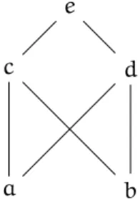
Figure 2.1: Hasse diagram of Example 2.1

Definition 2.1 (Partial order). Given a set S, a partial order≼ on S, is a binary relation (a subset of S× S) being:

• reflexive: ∀x ∈ S, x ≼ x;

• transitive: _{∀x, y, z ∈ S, x ≼ y ⇒ y ≼ z ⇒ x ≼ z;} • anti-symmetric: ∀x, y ∈ S, x ≼ y ⇒ y ≼ x ⇒ x = y

Definition 2.2 (Poset). When a set S, is equipped with a partial order≼, we say that (S, ≼) is a poset.

Definition 2.3 (Monotonicity). Given two posets (S1,≼1) and (S2,≼2), and a function f∈ S1 →

S2, f is said to be monotonous whenever∀x, y ∈ S1, x≼1 y⇒ f(x) ≼2 f(y).

Definition 2.4 (lower-bound, upper-bound, lub, glb). Given a poset (S,≼) and a subset X ⊆ S, we say that m (resp. M) is a lower (resp. upper) bound of X, whenever ∀x ∈ X, m ≼ x (resp. ∀x ∈ X, x ≼ M). We denote as X↓ _{(resp. X}↑_{) the subset of S of all lower bounds (resp. upper}

bounds) of X. Let m (resp. M) be a lower (resp. upper) bound of X, we say that m (resp. M) is the greatest lower bound (glb) (resp. least upper bound (lub)), whenever ∀m′ ∈ X↓, m′ ≼ m (resp. _∀M′_{∈ X}↑, M≼ M′_{). When such a lub (resp. glb) exists it is unique and will be denoted}

c

X (resp. bX).

A commonly used visual representation of posets (and this thesis will not fail to the rule) are Hasse diagrams, which we now succinctly present.

Definition 2.5 (Hasse diagrams). Given a poset (S,≼), we define the following directed graph (V, E), where:

• V = S

• E ={(x, y) | x ≼ y ∧ x 6= y ∧ ∀z ∈ S, x ≼ z ≼ y ⇒ z = x ∨ z = y}

Basically we have a transition between an element x and y if x ≼ y, but we remove transitions that can be inferred from the reflexive, and transitive, property of the order relation.

Remark 2.1. By the transitive and anti-symmetric property of the order relation we have that the graph is actually acyclic. Edges of a Hasse diagram are therefore represented visually by an edge going up from the smallest element of the two, to the biggest one.

Example 2.1 (Non existence of lub). Consider the following set S = {a, b, c, d, e} ordered by the relation ≼= {(a, a), (b, b), (c, c), (d, d), (e, e), (a, c), (a, d), (b, c), (b, d), (a, e), (b, e), (c, e), (d, e)}, represented by the Hasse diagram of Figure 2.1. We can see that the set {c, d} does not admit a greatest lower bound, however it admits a least upper boundb_{{c, d} = e}

Definition 2.6 (Chains). Given a poset (S,≼), a chain is a subset C of S such that: ∀x, y ∈ C, x ≼ y∨ y ≼ x. C is completely ordered.

Definition 2.7 (CPO). A poset (S,≼) is called a CPO if every chain of the poset admits a lub, it is then denoted (S,≼,b,⊥), where ⊥ =b∅.

(21)

12 CHAPTER 2. BACKGROUND – ABSTRACT INTERPRETATION ∅ {a} {a, b} {a, b, c} {a, b, c, d} {a, b, d} {a, c} {a, c, d} {a, d} {b} {b, c} {b, c, d} {b, d} {c} {c, d} {d}

Figure 2.2: Hasse diagram of Example 2.1

Definition 2.8 (Lattice). A poset (S,≼) is called a lattice when every subset of size 2 of S admits a lub and a glb, those are then denoted_{⋎ (for the lub) and ⋏ (for the glb). We then say that} (S,≼, ⋎, ⋏) is a lattice.

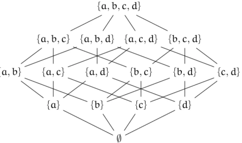
Definition 2.9 (Complete lattice). A lattice (S,≼, ⋎, ⋏) is said to be a complete lattice whenever every subset of X admits a glb. This implies that every subset of X admits a lub (and conversely). We then denote⊥ =b∅ and > =c∅, and say that (S, ≼, ⋎, ⋏, ⊥, >) is a complete lattice. Example 2.2 (Powerset lattice). For any given set X the powerset lattice (℘(X),∪, ∩, ∅, X) is a complete lattice. Figure 2.1 provides the Hasse diagram of the powerset lattice of the set {a, b, c, d}.

Definition 2.10 (Lifted lattice). Given a (complete) lattice (S,≼, ⋎, ⋏, ⊥, >) and a set X we can derive a new complete lattice: ((X→ (S \ {⊥})) ∪ ⊥, ≼, ⋎, ⋏, ⊥, >) where:

≼ ∆ ={(f, f′)| ∀x ∈ X, f(x) ≼ f′(x)} f⋎f ∆ = λx.f(x)⋎ f′(x) f⋏f ∆ = λx.f(x)⋏ f′(x) > ∆ = λx.>

and⊥ is a new element.

Remark 2.2. This last definition provides a way to lift a “value” lattice to an “environment” lattice by setting X to be a set of variables.

We now introduce vocabulary specific to abstract interpretation. Recall that instead of work-ing in the concrete world (C), our goal is to translate the computations to a simpler abstract world (A). In order to give a meaning to elements of the abstract world as abstractions of ele-ments from the concrete world, we define a concretization function, which is a function from the abstract world to the concrete one. We can then rely on the comparison operator provided by the concrete world to compare a concrete element with a concretized abstract element. As mentioned earlier, the notion of soundness is conveyed by the order relation of the concrete world, we will therefore say that an abstract element a is an sound abstraction of a concrete one c if the concretization of a is greater than c.

(22)

Definition 2.11 (Concretization, soundness, exactness). Given two posets (C,≼) and (A, v), a monotonic function γ∈ A → C is called a concretization function. Given c ∈ C and a ∈ A, we then say that:

• a is a sound abstraction of c whenever c≼ γ(a); • a is an exact abstraction of c whenever c = γ(a).

Even though the concretization is sufficient to reason about soundness (e.g. prove that an analyzer is sound in the sense that it considered the complete semantics of a program), we now define a stronger framework: Galois connections. The notion of Galois connection is used to link an abstract world and a concrete one, in addition to a concretization function, this provides an abstraction function. This function maps elements from the concrete world to elements from the abstract world. Moreover the equivalence from the next definition ensures that in a Galois connection the abstraction function provides the best possible sound abstraction (again for the order relation of the abstract world).

Definition 2.12 (Galois connections). Given two posets (C,≼) and (A, v), we say that the pair (α∈ C → A, γ ∈ A → C) is a Galois connection when:

∀a ∈ A, ∀c ∈ C, c ≼ γ(a) ⇔ α(c) v a We then write (C,≼) −−−→←−−−

α γ

(A,v)

Proposition 2.1 (Properties on Galois connections [CC77b]). Given a Galois connection (C,_{≼ ) −−−→}←−−−

α γ

(A,v) we have:

• γ and α are monotonic • _{∀c ∈ C, c ≼ γ ◦ α(c)} • ∀a ∈ A, α ◦ γ(a) v a

• γ◦ α ◦ γ = γ and α ◦ γ ◦ α = α

• _{∀c ∈ C, {a | c ≼ γ(a)} admits a glb and α(c) =}d_{{a | c ≼ γ(a)}} • ∀a ∈ A, {c | α(c) v a} admits a lub and γ(a) =b{c | α(c) v a} • Given two Galois connections (S1,≼1) −−−←−−−→

α1 γ1 (S2,≼2) and (S2,≼2) −−−←−−−→ α2 γ2 (S3,≼3) we have

the following Galois connection: (S1,≼1) −−−−−−←−−−−−−→ α2◦α1

γ1◦γ2

(S3,≼3)

• Given a Galois connection (C,_{≼) −−−→}←−−−

α γ

(A,v) between two lattices (C, ≼, ⋎, ⋏, ⊥c,>c) and

(A,v, t, u, ⊥a,>a), and a setV, we have a Galois connection between the two lifted posets

of Definition 2.10: ((X→ C \ {⊥c}) ∪ ⊥c,≼) −−−→←−−− α γ ((X→ A \ {⊥a}) ∪ ⊥a,v) where γ(f)=∆ { ⊥c if f =⊥a λs∈ X.γ(f(s)) otherwise α(f)=∆ { ⊥a if f =⊥c λs∈ X.α(f(s)) otherwise

2.2.2 An example of Galois connection: intervals [CC76]

We recall here the definition of the Galois connection between the lattice (℘(Z), ⊆, ∪, ∩, ∅, Z) and the interval lattice (see [CC76]). We define the set of intervals to be _I =∆ {[a; b] | a ∈ Z ∪ {−∞} ∧ b ∈ Z ∪ {∞} ∧ a ⩽ b} ∪ {⊥}. On I we define the concretization function γ such that

(23)

14 CHAPTER 2. BACKGROUND – ABSTRACT INTERPRETATION ⊥ . . . _{[−2; −2]} _{[−1; −1]} _{[0; 0]} _{[1; 1]} _{[2; 2]} . . . [−2; −1] [−1; 0] [0; 1] [1; 2] [−2; 0] [−1; 1] [0; 2] [−2; 1] [−1; 2] [−2; 2] ] −∞; −1] ] −∞; 0] ] −∞; 1] ] −∞; 2] [−2;∞[ [−1;∞[ [0;∞[ [1;∞[ . . . . . . ] −∞; ∞[

Figure 2.3: Hasse diagram of the interval lattice

γ([a; b]) ={x ∈ Z | a ⩽ x ⩽ b} and γ(⊥) = ∅. I is enriched with the following operators: v ∆

={([a; b], [c; d]) | c ⩽ a ∧ b ⩽ d} [a; b]t [c; d]= [min(a, c); max(b, d)]∆

[a; b]u [c; d]=∆ {

[max(a, c); min(b, d)] if max(a, c)⩽ min(b, d)

⊥ otherwise

> ∆

= [−∞; ∞]

(I, v, t, u, >, ⊥) is a complete lattice, Figure 2.3 represents its Hasse diagram. Moreover let us consider the function α∈ ℘(Z) → I defined by:

α(S) = {

[min(S); max(S)] if S6= ∅

⊥ otherwise

We then have the following Galois connection (℘(Z), ⊆) −−−→←−−−

α γ

(I, v). Note that we went from the world ℘(Z), the elements of which are not all machine representable, to the interval world I, the elements of which are machine representable. Obviously information was lost, consider for example the set 2_{Z which can not be precisely represented with an interval. Its most precise} abstraction is ] −∞; ∞[, representing Z ⊋ 2Z.

2.2.3 Operators, fixpoint theorems

The semantics of a transition system is defined using not only set-theoretic operations, but also operators, representing transition steps in the system. An operator is merely a function between two posets, we start here by providing some vocabulary on such functions.

Definition 2.13 (function properties).

• Continuity: Given two CPO (S_b 1,≼1) and (S2,≼2) (the lub of chains will be denoted resp. 1and

b

2), a function f∈ S1 → S2 is said to be continuous whenever for every chain C1

(24)

• Join-morphism: a function f between a lattice (S1,≼1,⋎1, . . . ) and a lattice (S2,≼2,⋎2, . . . )

is said to be a join-morphism when: ∀x, y ∈ A1, f(x⋎1y) = f(x)⋎2f(y). When A1 and

A2 are complete lattices and the property can be extended to arbitrary sets, we call f a

complete join morphism. A join morphism is monotonous, a complete join morphism is continuous.

We have seen how a concretization function is used to define a notion of sound abstraction of a concrete element. We now define a notion of sound operators. Informally a function fA_operating

on the abstract world is said to be a sound abstraction of its concrete counterpart f whenever the image of every abstract element is a sound abstraction of the image of the concretization of this element. This property is stable by composition, which ensures that an analyzer built as the composition of sound operators will itself be sound. Similarly a notion of exactness is defined. Definition 2.14 (Sound and exact abstraction of operators). Given a monotonic function γ from the poset (A,v) to the poset (C, ≼) and an operator f ∈ C → C. We say that fA _{is a sound}

abstraction of operator f whenever

∀x ∈ A, f(γ(x)) ≼ γ(fA_(x))

we say that is an exact abstraction of operator f whenever ∀x ∈ A, f(γ(x)) = γ(fA_(x))

Remark 2.3. When we are given a Galois connection between the concrete and abstract world: (C,≼) −−−→←−−−

α γ

(A,v), fA = α∆ ◦ f ◦ γ is a sound abstraction of f. Moreover it is the best possible abstraction of f in the sense that: if g is another sound abstraction of f then∀a ∈ A, fA_(a)_{v g(a).}

The definition of a semantics makes use of fixpoints (e.g. for the definition of the semantics of awhilestatement), more precisely it uses the notion of least fixed point, which is the smallest of all fixpoints. We provide here two fixpoint theorems that will ensure that the semantics is well-defined (there exists a least fixed point). Moreover as the definition of our abstract semantics will copy that of the original semantics we provide transfer theorems ensuring a fixpoint computed in the abstract world over-approximates the least fixed point from the original semantics. Definition 2.15 (Fixpoints). Given a poset (S,≼) and a function f ∈ S → S, we define:

• a fixpoint of f is an element x∈ S such that f(x) = x, we denote as fp(f) the set of all such fixpoints.

• lfp(f) denotes (when it exists) the least fixed point of f.

Theorem 2.1 (Tarski’s fixpoint theorem [Tar55]). If (S,≼, ⋎, ⋏, ⊥, >) is a non empty complete lattice and f is a monotonic function, then fp(f) is a non empty complete lattice, lfp(f) exists and is such that lfp(f) =c{x ∈ S | f(x) ≼ x}

Theorem 2.2 (Kleene’s fixpoint theorem [CC77b]). Given a CPO (S,≼,b,_{⊥), a continuous} func-tion f∈ S → S we have lfp(f) exists, {fn₍_{⊥) | n ∈ N} is a chain, and lfp(f) =}b_{fn₍_{⊥) | n ∈ N}.}

Theorem 2.3 (Tarski’s fixpoint approximation [Cou97]). Given a complete lattice (C,≼, ⋎, ⋏, ⊥c,>c), a poset (A,v), a concretization function γ from A to C, f a monotonic operator on C, g

an operator on A that is a sound approximation of f with respect to γ, then∀a ∈ A, g(a) v a ⇒ lfp(f)≼ γ(a).

Theorem 2.4 (Kleene’s fixpoint approximation [Cou97]). Given a CPO (C,≼,b,⊥c), a poset

with minimal element (A,v, ⊥a), a concretization function γ from A to C, f a continuous operator

on C, g an operator on A that is a sound approximation of f with respect to γ, if the sequence {gi₍_⊥

a)| i ∈ N} has a least upper bound l =

F {gi₍_⊥

(25)

2.2.4 Widening

In the introductory remarks to this chapter we underlined four difficulties encountered while trying to compute the concrete semantics. To this point we provided an answer to the first three by translating the problem to an abstract world. However there remains the problem that the least fixed point used in the concrete may not be computed in finitely many steps in the abstract. As we will see in the next section, following Kleene’s fixpoint theorem, we compute over-approximations of fixpoints of functions f by considering the iterates (fAi₍_⊥))

i∈N, where

fAis a sound approximation of operator f. The sequence (fAi₍_⊥))

i∈Nwill often be increasing.

Whenever the abstract world has finite height (meaning that there exists no infinite sequence (yi)i∈Nsuch that∀i, yiv yi+1and yi6= yi+1) the iterates (fAi(⊥))i∈Nconverges. However in

all abstractions considered in this thesis, the abstract lattice will have infinite height, therefore the sequence (fAi₍_⊥))

i∈N is not ensured to converge. For this reason we define a widening

operator, the goal of which is to stabilize sequences.

Definition 2.16 (Widening operator). Given a poset (A,v) we say that a binary operator ▽ ∈ A× A → A is a widening operator if:

1. ∀x, y ∈ A, x v x▽y ∧ y v x▽y

2. for all sequences (xi)i∈N∈ ANthe sequence (yi)i∈N ∈ ANdefined by (y0= x0)∧ (yi+1 =

yi▽xi+1) satisfies∃N ∈ N, ∀k ⩾ N, yk= yN

Theorem 2.5 (Widening ensures convergence [CC77b]). Given a complete lattice C, a poset A with minimal element⊥A, a concretization function γ from A to C, a monotonic operator f on C,

an operator g on A that is a sound approximation of f with respect to γ, then the sequence (yi)i∈N

defined by:

y0 =⊥A

yi+1 = yi▽g(yi)

is such that_{∃N ∈ N, ∀k ⩾ N, y}_k= yN. Moreover for such a N, we have lfp(f)≼ γ(yN).

2.3 Abstract Interpretation

2.3.1 By example

As abstract interpretation is a framework easing the development of static analyzers by providing sufficient conditions to ensure the soundness of the analysis, we show here an example of static analyzer defined by abstract interpretation. Let us consider a modified version of register ma-chines as toy language for this section. The reason we chose to present register machine as toy language is the fact that numerical operations are limited to incrementation and decrementa-tion. Therefore we do not have to deal with the definition of the evaluation of expressions. This language will be denoted as RM in the remainder of this section. The different points presented in the following are the classical steps followed by the definition of an abstract interpreter.

Syntax of the language. We start by providing the syntax of the language. We assume given a finite non empty set of variables (the registers) denotedR. We denote as stmt the set of all

(26)

2.3. ABSTRACT INTERPRETATION 17

statements from our language, defined by the following grammar.

stmt=∆ |while (r!=0) {stmt} r∈ R |if (r!=0) {stmt} else {stmt} r∈ R |skip |stmt;stmt | r++ r∈ R | r-- r∈ R

Memory state. The semantics of the language will operate on sets of states which are maps assigning an integer value to each of the registers. We denote asD the set of all such sets of maps: _D= ℘(∆ R → Z).

Semantics of atomic statements. As mentioned in the introductory remarks to this section, the definition of the semantics requires the definition of the transfer functions for atomic statements. Given an atomic statementstmtwe denote asSJstmtK ∈ D → D the transfer function associated to statementstmt. SJr==0K= λR∆ ∈ D.{ρ | ρ ∈ R ∧ ρ(r) = 0} SJr!=0K= λR∆ ∈ D.{ρ | ρ ∈ R ∧ ρ(r) 6= 0} SJr++K= λR∆ ∈ D.{ρ[r 7→ ρ(r) + 1] | ρ ∈ R} SJr--K= λR∆ ∈ D.{ρ[r 7→ ρ(r) − 1] | ρ ∈ R} SJskipK= λR∆ ∈ D.R

Semantics of compound statements. Now that we have provided a mathematical definition of the semantics of atomic statements, we define by induction on the syntax, the semantics of compound statements. As mentioned before, these definitions rely on the use of the mathemat-ical set union and smallest fixed points.

SJwhile (r!=0) {stmt}K= λR∆ ∈ D.SJr==0K(lfp(λS ∈ D.R ∪ SJstmtK ◦ SJr!=0K(S)))

SJif (r!=0) {stmtt} else {stmte}K= λR∆ ∈ D.SJstmttK ◦ SJr!=0K(R) ∪ SJstmteK ◦ SJr==0K(R)

SJstmt1;stmt2K=∆ SJstmt2K ◦ SJstmt1K

We mentioned that any powerset is a complete lattice. In particular hereD is a complete lattice, and we can show that for every statementstmtSJstmtK is a complete join-morphism. It follows that for every R∈ D and for everystmt∈stmtthe function F= λS∆ ∈ D.R ∪ SJstmtK ◦ SJr!=0K(S) ∈

D → D is a complete join-morphism. By application of both Theorem 2.1 and Theorem 2.2 we get that F admits a least fixed point. Therefore our semantics is well-defined.

Abstract domain. The first step in building a static analyzer by abstract interpretation is the definition of an abstract domain. An abstract domain is a structure providing all the operators re-quired for the definition of an abstract semantics. We recall that the abstract semantics is defined by following the definition of the concrete semantics and replacing some of the uncomputable operators by computable, over-approximating ones. Moreover as the least fixed point might not be reached (via Kleene’s theorem) in a finite number of iterations, we ask abstract domains to provide an operator accelerating convergence, denoted_{▽. An abstract domain therefore} pro-vides:

(27)

• A lattice (D♯_,_{v, t, u, ⊥, >);}

• A Galois connection with the concrete domain (D, ⊆) −−−→←−−−

α γ

(D♯_,_v);

• Abstract transformers for the atomic statements of the language, denoted as _S♯_J_stmt_{K ∈}

D♯_{→ D}♯_: _S♯_Jr₌₌₀_{K, S}♯_Jr_!=₀_{K, S}♯_Jr₊₊_{K, S}♯_Jr_--_K;

• A widening operator▽ ∈ D♯_{× D}♯_{→ D}♯_.

Moreover in order to ensure soundness and computability of the overall analysis, produced by the composition of such operators, we require the following to hold:

• t is a sound over-approximation of the union operator ∪ (we extend Definition 2.14):

∀R♯ 1, R ♯ 2 ∈ D♯, γ(R ♯ 1)∪ γ(R ♯ 2)⊆ γ(R ♯ 1t R ♯ 2)

• For all atomic statementsstmt,S♯_J_stmt_{K is a sound abstraction of operators SJ}_stmt_{K, in the}

sense of Definition 2.14;

• Elements fromD♯_{are machine representable;}

• ▽, t, and S♯_J_stmt_{K for any}_stmt_{are computable operators.}

Example continued: the interval domain. Let us now define an abstract domain for the RM language. Our first abstraction will be to lose the relationality of the concrete worldD = ℘(R → Z). We have shown that (℘(Z), ⊆, ∪, ∩, ∅, Z) is a complete lattice. We lift this lattice using Definition 2.10, to a lattice L1 = (R → ℘(Z) \ {∅}) ∪ {⊥}, ⊆, ∪, ∩, ⊥, >). We now define a Galois

connection between the concrete world and this lattice:

℘(R → Z) −−−→←−−− α1 γ1 ((R → ℘(Z) \ {∅}) ∪ {⊥}, ⊆) γ1(m) = { ∅ if m =⊥ {ρ ∈ R → Z | ∀r ∈ R, ρ(r) ∈ m(r)} otherwise α1(R) = { ⊥ if R =∅ λr∈ R.{ρ(r) | ρ ∈ R} otherwise

Note that this abstraction looses relations between values in registers. As an example consider the set of environments R = {(r1 7→ 1, r2 7→ 0), (r1 7→ 0, r2 7→ 1)}, we have α(R) = (r1 7→

{0, 1}, r2 7→ {0, 1}) and therefore γ ◦ α(R) = {(r1 7→ 1, r2 7→ 0), (r1 7→ 0, r2 7→ 1), (r1 7→ 0, r2 7→

0), (r1 7→ 1, r2 7→ 1)}.

Moreover we have shown in Section 2.2.2 a Galois connection between ℘(Z) and I the set of intervals ofZ. By lifting this Galois connection using Proposition 2.1 and Definition 2.10 we get a Galois connection between the lattice L1 and the lattice ((R → (I \ {⊥}) ∪ {⊥}, v, t, u, >, ⊥),

we denoteD♯_{= (R → (I \ {⊥}) ∪ {⊥}}∆

((R → ℘(Z) \ {∅}) ∪ {⊥}, ⊆) −−−→←−−−

α2

γ2

(D♯_,_v)

By the composability result provided in Proposition 2.1 we get a Galois connection between our concrete worldD and our abstract world D♯_{. Moreover please note that as}_{R is finite, elements}

from our abstract world are machine representable and our abstract operators are computable. Let us now define sound abstract transformers on_D♯_{, over-approximating the semantics of the}

(28)

2.3. ABSTRACT INTERPRETATION 19 S♯_Jr₌₌₀_K ∆ = λR♯∈ D♯. { ⊥ if R♯₌_{⊥ ∨ 0 /∈ R}♯_(r) R♯[r7→ [0; 0]] otherwise S♯_Jr_!=₀_K ∆ = λR♯∈ D♯.        ⊥ if R♯₌_{⊥ ∨ R}♯_{(r) = [0; 0]} R♯[r7→ [1; a]] else if R♯_{(r) = [0; a]}

R♯[r7→ [a; −1]] else if R♯(r) = [a; 0]

R♯ otherwise

S♯_Jr₊₊_K ∆

= λR♯∈ D♯. {

⊥ if R♯₌_⊥

R♯[r7→ [a + 1; b + 1]] otherwise when R♯(r) = [a; b] S♯_Jr_--_K ∆

= λR♯∈ D♯. {

⊥ if R♯₌_⊥

R♯[r7→ [a − 1; b − 1]] otherwise when R♯(r) = [a; b]

In order not to make the previous definitions too cumbersome, we assumed that ∞ ± 1 = ∞ and −∞ ± 1 = −∞. All above abstract operators are sound and or the best possible abstract operators that can be associated to their concrete counterpart.

We now provide a widening operator for the interval domain. As for the other set abstract operators, we define_{▽ as a lifting to maps of the following operator:}

[a; b]▽0[c; d]= [∆ { −∞ if c < a a otherwise ; { ∞ if d > b b otherwise ]

Finally please note that all soundness and computability conditions are met by our definitions. Abstract semantics. Now that we have defined an abstract domain, an abstract semantics can be automatically defined by following the definition of the concrete semantics and replacing every operator by its abstract counterpart. In the following_{v, u, t, ⊥, > denotes the abstract} operator on the lifted interval abstract domain.

S♯_J_while ₍_r_!=₀_{) {stmt}}_K ∆ = λR♯∈ D♯.S♯_Jr₌₌₀_{K( lim} n→∞F n₍_⊥)) with F(S♯_{) = S}♯_▽(R♯_{t S}♯_J_stmt_{K ◦ S}♯_Jr_!=₀_K(S♯₎₎ S♯_J_if ₍_r_!=₀_{) {stmt} t} else {stmte}K ∆ = λR♯∈ D♯._S♯_J_stmt tK ◦ S♯Jr!=0K(R♯) t S♯_J_stmt eK ◦ S♯Jr==0K(R♯) S♯_J_stmt 1;stmt2K=∆ S♯Jstmt2K ◦ S♯Jstmt1K S♯_J_skip_K ∆ = λR♯∈ D♯.R♯

Using the soundness and computability of abstract operators for atomic statements and for abstract set operators, the stabilizing property of the widening operator, and the fixpoint transfer theorems, we can show that the composition of these operators in the definition of our abstract semantics is sound and computable.

Theorem 2.6 (Soundness and computability). For every statementstmt,_S♯_J_stmt_{K is a sound and}

computable abstraction of operator_SJstmtK.

Application. Let us consider Program 2.1 written in RM where_{R = {}a,b,c}. We can show that SJaddK ∈ D → D is such that ∀x, y ∈ N, SJaddK({(a7→ x,b7→ y,c7→ 0)}) = {(a7→ 0,b7→ 0,c7→ x + y)}. Moreover if aor b is initially negative, then the set of reachable states at the end of