HAL Id: cel-01393191
https://hal.archives-ouvertes.fr/cel-01393191
Submitted on 7 Nov 2016HAL is a multi-disciplinary open access archive for the deposit and dissemination of sci-entific research documents, whether they are pub-lished or not. The documents may come from teaching and research institutions in France or abroad, or from public or private research centers.
L’archive ouverte pluridisciplinaire HAL, est destinée au dépôt et à la diffusion de documents scientifiques de niveau recherche, publiés ou non, émanant des établissements d’enseignement et de recherche français ou étrangers, des laboratoires publics ou privés.
Minimal Surfaces Embedded in Euclidean Space
Lucky Anetor
To cite this version:
Lucky Anetor. Minimal Surfaces Embedded in Euclidean Space. Master. Differential Geometry, United States. 2016. �cel-01393191�
Minimal Surfaces Embedded in Euclidean Space
Lucky Anetor ∗Department of Mechanical Engineering Nigerian Defence Academy, Kaduna, Nigeria
Abstract
The main objective of this work is to present a brief tutorial on minimal surfaces. Furthermore, a great deal of effort was made to make this tutorial as accessible and self-contained as possible. The intention of the materials presented in this work is to give some motivations for beginners to go further in the study of the exciting field of minimal surfaces in three dimensional Euclidean space and in other ambient spaces. The minimal surface equation was derived and it was used to generate some minimal surfaces on application of the appropriate boundary conditions. Further-more, the Weierstrass-Enneper equation was derived, this was again used to generate both the classical and modern minimal surfaces. Some advantages and shortcomings of the Weierstrass-Enneper equations were highlighted. Finally, it was pointed out that for generalized Gauss map of minimal surfaces in Rn, where n > 3, one does not have a unique unit normal N anymore.
Keywords: Minimal Surfaces, Mean Curvature, Gauss map and Weierstrass-Enneper representation
1
Introduction
In 1744, Euler posed and solved the problem of finding the surfaces of revolution that minimize area. The only solution found then was the catenoid. After about eleven years, in a series of letters to Euler, Lagrange, at age 19, discussed the problem of finding a graph over a region in the plane, with prescribed boundary values, that was a critical point for the area function. He wrote down what would now be called the Euler-Lagrange equation for the solution (a second-order, nonlinear and elliptic partial differential equation), but he did not provide any new solutions. In 1776, Meusnier showed that the helicoid was also a solution. Equally important, he gave a geometric interpretation of the Euler-Lagrange equation in terms of the vanishing of the mean of the principal curvatures of the surface, a quantity now known, after a suggestion of Sophie Germain, as the mean curvature [1–3].
Minimal surfaces are of interest in various branches of mathematics, science and engineering. In calculus of variations they could appear as surfaces of least or maximum area, (where the minimal surface occur with the least area, it is called the stable minimal surfaces), in differential geometry, as surface whose mean curvature is everywhere zero (vanishes). In gas dynamics, the equations of minimal surfaces is interpreted as the potential equation of a hypothetical gas, which yields flows closely approximating adiabatic flows of low Mach number. This interpretation given by Chaplygin has been used extensively in aerodynamic literatures [4]. In the general theory of partial differential
equations, the minimal surface equations appears as the simplest nonlinear equation of the elliptic type. It has the defining property that every sufficiently small piece of it (small enough, say, to be a graph over some plane) is the surface of least area among all surfaces with the same boundary. The simplest minimal surface is the flat plane, but other minimal surfaces are far from simple [5]. Minimal surfaces are realized in the physical world by soap films spanning closed curves, and they appear as interfaces where the pressure is the same on either side. Finding a surface of least area spanning a given contour is known as the Plateau problem, after the nineteenth-century Belgian physicist Felix Plateau, who posed the problem of finding a mathematical description of these solutions (and, by implication, a proof that they exist).
Surfaces that locally minimize area have been extensively used to model physical phenomena, in-cluding soap films, black holes, crystals, polymer compounds, protein folding, etc [6]. Although the mathematical field started in the 1740s it has recently become an area of active mathemati-cal and scientific study, specifimathemati-cally in the areas of molecular engineering, materials science, and nano-technology because of their many anticipated applications.
The objective of this work is to make this tutorial as accessible and self-contained as possible so that the materials will be appealing to beginners who are interested in the exciting field of minimal surfaces. This work is divided into five sections. Section 1 gives a brief introduction into the field of minimal surfaces. In section 2, a literature survey of recent works on minimal surfaces are presented. Some of the basics of differential geometry of surfaces which are relevant to this work are discussed in section 3. In section 4, examples of the classical minimal surfaces, namely, the helicoid, catenoid and the Scherks surface were presented. These surfaces were derived by imposing different conditions (algebraic and geometric) on the minimal surface elliptic partial differential equation. The Weierstrass-Enneper representation of minimal surfaces was covered in section 5 and the results were used to derive the equations for both the classical and modern minimal surfaces. Finally, some concluding remarks were stated.
2
Literature Review
The bulk of the results of the research that have been done in this field may be found in the works of Douglas [7, 8] and in the books of Rad´o, Courant and Osserman, [9–11] respectively. Of all
the research that has been carried out in the field of minimal surfaces, Bernstein’s work offered a perspective which was different from those of Rad´o and Courant [9, 10] in that he considered
minimal surfaces mainly from the point of view of partial differential equations. Recent efforts in the study of minimal surfaces have been in the areas of generalizations to higher dimensions, Riemannian spaces, wider classes of surfaces; and partly in the direction of many new results in the classical case. Most recent results on minimal surfaces, focusing on the classification and structure of embedded minimal surfaces and the stable singularities were discussed in [12]. The survey of recent spectacular successes in classical minimal surface theory were presented by [13]. For more information on the theory of minimal surfaces, the interested reader should consult the survey papers [14–17].
3
The Basics of Differential Geometry of Surfaces
What is a surface? A precise answer cannot really be given without introducing the concept of a manifold. An informal answer is to say that a surface is a set of points in R3such that, for every point
p on the surface, there is a small (perhaps very small) neighborhood U of p that is continuously
locally, unless the point p is singular, the surface looks like a plane. Properties of surfaces can be classified into local properties and global properties. In the older literature, the study of local properties was called geometry in the small, and the study of global properties was called geometry in the large. Local properties are the properties that hold in a small neighborhood of a point on a surface. Curvature is a local property. Local properties can be studied more conveniently by assuming that the surface is parameterized locally. Therefore, it is relevant and useful to study parameterized patches.
Another more subtle distinction should be made between intrinsic and extrinsic properties of a surface. Roughly speaking, intrinsic properties are properties of a surface that do not depend on the way the surface is immersed in the ambient space, whereas extrinsic properties depend on properties of the ambient space. For example, we will see that the Gaussian curvature is an intrinsic concept, whereas the normal to a surface at a point is an extrinsic concept.
In this section, we shall focus exclusively on the study of local properties.
1. By studying the properties of the curvature of curves on a surface, we will be led to the First and the Second Fundamental Form of a surface.
2. The study of the normal and of the tangential components of the curvature will lead to the normal curvature and to the geodesic curvature. But we shall not be treating geodesic curvature, since the objective of this report is to study minimal surfaces.
3. We will study the normal curvature, and this will lead us to principal curvatures, principal directions, the Gaussian curvature, and the mean curvature.
4. The study of the variation of the normal at a point will lead to the Gauss map and its derivative.
3.1 Parameterized Surfaces
In this section, we consider exclusively surfaces immersed in the affine space R3. In order to be able to define the normal to a surface at a point, and the notion of curvature, we assume that some inner product is defined on R3.
Unless specified otherwise, we assume that this inner product is the standard one, that is,
⟨(x1, x2, x3) , (y1, y2, y3)⟩ = x1y1+ x2y2+ x3y3 (3.1)
A surface is a map X : D → R3, where D is some open subset of the plane R2, and where X is at least C3-continuously differentiable. Actually, we will need to impose an extra condition on a surface X so that the tangent and the normal planes at any point p are defined. Again, this leads us to consider curves on X.
A curve C on X is defined as a map
C : t → X(u(t), v(t)) (3.2)
where u and v are continuous functions on some open interval I contained in D. We also assume that the plane curve t → (u(t), v(t)) is regular, that is,
( du(t) dt , dv(t) dt ) ̸= (0, 0) (3.3)
for all t∈ I.
For example, the curves v → X(u0, v) for some constant u0 are called u-curves, and the curves
u → X(u, v0) for some constant v0 are called v-curves. Such curves are also called the coordinate
curves.
The tangent vector dC(t)dt toC at t can be computed using the chain rule
dC(t) dt = ∂X(u(t), v(t)) ∂u · du(t) dt + ∂X(u(t), v(t)) ∂v · dv(t) dt (3.4)
are vectors, but for simplicity of notation, we omit the vector symbol in these expressions. It is customary to use the following abbreviations such that the partial derivatives
∂X(u(t), v(t))
∂u and
∂X(u(t), v(t)) ∂v
are denoted by Xu(t) and Xv(t), or even by Xu and Xv, respectively and the derivatives
dC(t) dt , du(t) dt and dv(t) dt
are denoted by ˙C(t), ˙u(t) and ˙v(t) or even as ˙C, ˙u and ˙v. When the curve C is parameterized by arc length s, we denote
dC(s) ds , du(s) ds and dv(s) ds
by C′(s), u′(s), and v′(s), or even as C′, u′, and v′. Thus, we reserve the prime notation to the case where the parametrization of C is by arc length.
Note that it is the curve C : t → X(u(t), v(t)) which is parameterized by arc length, not the curve
t→ (u(t), v(t)).
Using these notations, ˙C(t) is expressed as follows: ˙
C(t) = Xu(t) ˙u(t) + Xv(t) ˙v(t) (3.5)
or simply as
˙
C = Xuu + X˙ v˙v
Now, if we want ˙C ̸= 0 for all regular curves t → (u(t), v(t)), we must require that Xu and Xv be linearly independent.
Equivalently, we must require that the cross-product Xu× Xv ̸= 0, that is, be non-null.
Definition A surface patch X, for short a surface X, is a map X :D → R3, whereD is some open
subset of the plane R2 and where X is at leastC3-continuously differentiable.
We say that the surface X is regular at (u, v)∈ D if and only if Xu× Xv ̸= 0, and we also say that
p = X(u, v) is a regular point of X. If Xu× Xv = 0, we say that p = X(u, v) is a singular point of X.
The surface X is regular on D if and only if Xu× Xv ̸= 0, for all (u, v) ∈ D. The subset X(D) of R3 is called the trace of the surface X.
Remark: It is often desirable to define a (regular) surface patch X :D → R3 whereD is a closed
subset of R2. IfD is a closed set, we assume that there is some open subset U containing D and such that X can be extended to a (regular) surface over U (that is, that X is at least C3-continuously differentiable).
Given a regular point p = X(u, v), since the tangent vectors to all the curves passing through a given point are of the form
Xuu + X˙ v ˙v (3.6)
it is obvious that they form a vector space of dimension two isomorphic to R2, called the tangent space at p and denoted as Tp(X).
Note that (Xu, Xv) is a basis of this vector space Tp(X).
The set of tangent lines passing through p and having some tangent vector in Tp(X) as direction is an affine plane called the affine tangent plane at p.
Geometrically, this is an object different from Tp(X), and it should be denoted differently (perhaps as ATp(X)).
The unit vector
Np=
Xu× Xv
|Xu× Xv|
(3.7) is called the unit normal vector at p, and the line through p of direction Np is the normal line to X at p. This time, we can use the notation Np for the line, to distinguish it from the vector Np. The fact that we are not requiring the map X defining a surface X : D → R3 to be injective may cause problems. Indeed, if X is not injective, it may happen that p = X(u0, v0) = X(u1, v1) for
some (u0, v0) and (u1, v1) such that (u0, v0)̸= (u1, v1). In this case, the tangent plane Tp(X) at p is not well defined. Indeed, we really have two pairs of partial derivatives (Xu(u0, v0) , Xv(u0, v0))
and (Xu(u1, v1), Xv(u1, v1)), and the planes spanned by these pairs could be distinct.
In this case, there are really two tangent planes T(u0, v0)(X) and T(u1, v1)(X) at the point p where X
has a self-intersection. Similarly, the normal Np is not well defined, and we really have two normals N(u0, v0) and N(u1, v1) at p.
We could avoid this problem entirely by assuming that X is injective (homeomorphic). This will rule out many surfaces that come up in practice.
If necessary, we use the notation T(u, v)(X) or N(u, v) which removes possible ambiguities. However, it is a more cumbersome notation, and we will continue to write Tp(X) and Np, being aware that this may be an ambiguous notation, and that some additional information is needed.
The tangent space may also be undefined when p is not a regular point. For example, consider the surface X = (x(u, v), y(u, v), z(u, v)) defined such that
x = u(u2+ v2), y = v(u2+ v2) and z = u2v− v3/3 (3.8)
note that all the partial derivatives at the origin (0, 0) are zero. Thus, the origin is a singular point of the surface X. Indeed, one can check that the tangent lines at the origin do not lie in a plane.
It is interesting to see how the unit normal vector Np changes under a change of parameters. Assume that u = u(r, s) and v = v(r, s), where (r, s)→ (u, v) is a diffeomorphism. By the chain rule Xr× Xs = ( Xu ∂u ∂r + Xv ∂v ∂r ) × ( Xu ∂u ∂s + Xv ∂v ∂s ) = ( ∂u ∂r ∂v ∂s − ∂u ∂s ∂v ∂r ) Xu× Xv = det ( ur us vr vs ) Xu× Xv = ∂(u, v) ∂(r, s) Xu× Xv (3.9)
denoting the Jacobian determinant of the map, (r, s) → (u, v) as ∂(u, v)/∂(r, s). Then, the rela-tionship between the unit vectors N(u, v) and N(r, s) is
N(r, s)= N(u, v) sign∂(u, v)
∂(r, s) (3.10)
We will therefore restrict our attention to changes of variables such that the Jacobian determinant ∂(u, v)
∂(r, s) is positive.
Notice also that the condition Xu× Xv ̸= 0 is equivalent to the fact that the Jacobian matrix of the derivative of the map X : D → R3 has rank 2, that is, the derivative DX(u, v) of X at (u, v) is injective.
Indeed, the Jacobian matrix of the derivative of the map (u, v)→ X(u, v) = (x(u, v), y(u, v), z(u, v))
is
xyuu xyvv
vu zv
and Xu× Xv ̸= 0 is equivalent to saying that one of the minors of order 2 is invertible. That is,
xuyv− xvyu̸= 0, xuzv− xvvu ̸= 0 and yuzv− yvvu ̸= 0 (3.11) Thus, a regular surface is an immersion of an open set of R2 into R3.
To a great extent, the properties of a surface can be investigated by studying the properties of curves on the surface. One of the most important properties of a surface is its curvature. A gentle way to introduce the curvature of a surface is to study the curvature of a curve on a surface. For this, we will need to compute the norm of the tangent vector to a curve on a surface. This will lead us to the first fundamental form.
3.2 The First Fundamental Form (Riemannian Metric)
Given a curveC on a surface X, we first compute the element of arc length of the curve C. For this, we need to compute the square norm of the tangent vector ˙C(t).
The square norm of the tangent vector ˙C(t) to the curve C at p is
| ˙C|2=⟨(X
where ⟨⋆ , ⋆⟩ is the inner product in R3, and thus
| ˙C|2=⟨X
u, Xu⟩ ˙u2+ 2 (⟨Xu, Xv⟩) ˙u ˙v + ⟨Xv, Xv⟩ ˙v2 (3.13) Following common usage, we let
E =⟨Xu, Xu⟩, F =⟨Xu, Xv⟩, and G =⟨Xv, Xv⟩ therefore
| ˙C|2 = E ˙u2+ 2F ˙u ˙v + G ˙v2 (3.14)
Euler obtained this formula in 1760. Thus, the map
(x, y)→ Ex2+ 2F xy + Gy2
is a quadratic form on R2, and since it is equal to | ˙C|2, it is positive definite. This quadratic form plays a major role in the theory of surfaces, and deserves a formal definition.
Definition Given a surface X, for any point p = X(u, v) on X, and letting
E =⟨Xu, Xu⟩, F =⟨Xu, Xv⟩, and G =⟨Xv, Xv⟩
the positive definite quadratic form (x, y)→ Ex2+ 2F xy + Gy2 is called the First Fundamental Form of X at p. It is often denoted as Ip and in matrix form, we have
Ip(x, y) = (x, y) ( E F F G ) ( x y ) (3.15) Since the map (x, y)→ Ex2+ 2F xy + Gy2is a positive definite quadratic form, we must have E ̸= 0 and G̸= 0.
Then, we can write
Ex2+ 2F xy + Gy2= E ( x + F Ey )2 + EG− F 2 E y 2
Since this quantity must be positive, we must have E > 0, G > 0, and also EG− F2 > 0.
The symmetric bilinear form ϕI associated with I is an inner product on the tangent space at p, such that ϕI((x1, y1) , (x2, y2)) = (x1, y1) ( E F F G ) ( x2 y2 ) (3.16) This inner product is also denoted as ⟨(x1, y1) , (x2, y2)⟩p
The inner product ϕI can be used to determine the angle of two curves passing through p, that is, the angle θ of the tangent vectors to these two curves at p. We have
cos θ = √⟨( ˙u1, ˙v1), ( ˙u2, ˙v2)⟩
I( ˙u1, ˙v1)
√
I( ˙u2, ˙v2)
For example, the angle θ between the u-curve and the v-curve passing through p (where u or v is constant) is given by
cos θ = √F
EG
Thus, the u-curves and the v-curves are orthogonal if and only if F (u, v) = 0 on D. Remarks: (1)Since ( ds dt )2 =| ˙C|2 = E ˙u2+ 2F ˙u ˙v + G ˙v2
represents the square of the element of arc length of the curve C on X, and since du = ˙udt and
dv = ˙vdt, one often writes the first fundamental form as
ds2 = E du2+ 2F du dv + G dv2 (3.18) Thus, the length l(pq) of an arc of curve on the surface joining p = X(u(t0), v(t0)) and q =
X(u(t1), v(t1)), is l(p, q) = ∫ t1 t0 √ E ˙u2+ 2F ˙u ˙v + G ˙v2 dt (3.19)
One also refers to ds2= E du2+ 2F du dv + G dv2 as a Riemannian metric. The symmetric matrix associated with the first fundamental form is also denoted as
(
g11 g12
g21 g22
)
where g12= g21
(2) As in the previous section, if X is not injective, the first fundamental form Ip will not be well defined. What is well defined is I(u, v). In some sense, this is even worse, since one of the main themes of differential geometry is that the metric properties of a surface (or of a manifold) are captured by a Riemannian metric. We will not be too bordered about this, since we can always assume that X injective.
(3) Using the identity,|Xu|2|Xv|2 = (⟨Xu, Xv⟩)2+|Xu× Xv|2 for any two vectors Xu, Xv ∈ R3, it can be shown that the element of area dA on a surface X is given by
dA =|Xu× Xv| du dv = √
EG− F2du dv (3.20)
We just discovered that, contrary to a flat surface where the inner product is the same at every point, on a curved surface, the inner product induced by the Riemannian metric on the tangent space at every point changes as the point moves on the surface. This fundamental idea is at the heart of the definition of an abstract Riemannian manifold. It is also important to observe that the first fundamental form of a surface does not characterize the surface.
For example, it is easy to see that the first fundamental form of a plane and the first fundamental form of a cylinder of revolution defined by
X(u, v) = (cos u, sin u, v) (3.21)
Thus ds2= du2 + dv2, which is not surprising. A more striking example is that of the helicoid and
of the catenoid.
The helicoid is the surface defined over R× R such that
x = u1cos v1
y = u1sin v1
z = v1 (3.22)
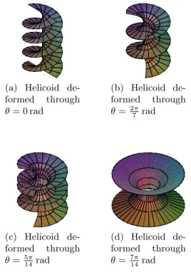
This is the surface generated by a line parallel to the xOy plane, touching the z axis, and also touching an helix of axis Oz. It is easily verified that (E, F, G) = (1, 0, u21+ 1). Figures 1a and 1b show a portion of helicoid corresponding to (0≤ v1 ≤ 2π) and (−2 ≤ u1 ≤ 2).
The catenoid is the surface of revolution defined over R× R such that
x = cosh u2cos v2
y = cosh u2sin v2
z = u2 (3.23)
It is the surface obtained by rotating a catenary about the z-axis. It is easily verified that (E, F, G) = (cosh2u2, 0, cosh2u2). Figures 1c and 1d show a catenoid corresponding to (0 ≤
v2 ≤ 2π) and (−2 ≤ u2 ≤ 2).
We can make the change of variables u1 = sinh u3, v1 = v3, which is bijective and whose Jacobian
determinant is cosh u3, which is always positive, obtaining the following parametrization of the
helicoid:
x = sinh u3cos v3
y = sinh u3sin v3
z = v3 (3.24)
It is easily verified that (E, F, G) = (cosh2u3, 0, cosh2u3), showing that the helicoid and the
catenoid have the same first fundamental form. What is happening is that the two surfaces are locally isometric (roughly, this means that there is a smooth map between the two surfaces that preserves distances locally). Indeed, if we consider the portions of the two surfaces corresponding to the domain R× (0, 2π), it is possible to deform isometrically the portion of helicoid into the portion of catenoid (note that by excluding 0 and 2π, we made a slit in the catenoid (a portion of meridian), and thus we can open up the catenoid and deform it into the helicoid). This is illustrated in Figure 2.
We will now show how the first fundamental form relates to the curvature of curves on a surface.
3.3 Normal Curvature and the Second Fundamental Form
Since the cross product of two vectors is always perpendicular to each of the vectors themselves, it follows that we can always find a unit normal vector N to the tangent plane of a surface M parameterized by X(u, v), such that
N = Xu× Xv
|Xu× Xv|
(3.25) The normal curvature in the tangent direction w is defined as follows:
Take the plane determined by the chosen unit direction vector w and the unit normal N, denoted by P = plane(w, N), and intersect this plane with surface M . The intersection is a curve α(s) (which we can assume is a unit speed curve). For unit speed curves, the curvature, κ(s) is |α′′(s)|. Therefore the curvature in the normal direction should just be the projection of the acceleration onto the normal direction. In order words,
Definition For a unit tangent vector w, the normal curvature in the w-direction is defined as
k(w) =⟨α′′(s) , N⟩, where the derivatives are taken along the curve with respect to s. Lemma 3.1 If α(s) is a curve in M , then ⟨α′′(s) , N⟩ = − ⟨α′(s) , N′⟩.
Proof We know that α′(s) is a tangent vector and N is normal to the tangent plane, so⟨α′(s) , N⟩ = 0. On differentiating both sides of this equation, we have
(⟨α′(s) , N⟩)′ = 0 =⇒ ⟨α′′(s) , N⟩ + ⟨α′(s) , N′⟩ = 0 =⇒ ⟨α′′(s) , N⟩ = − ⟨α′(s) , N′⟩ Remark
Again, the derivatives were taken along the curve with respect to s. To take N′, we again use the chain rule to get
N′ = Nuu′+ Nvv′ with u′ =
du ds, v
′ = dv
ds
We interpret⟨α′′(s) , N⟩ as the component of acceleration due to the bending of M. Recall that we assumed that α has unit speed so that the magnitude of α′(s) does not affect our measurement. By Lemma 3.1 and Remark 1, we have
k(w) = − ⟨α′(s) , N′⟩
= − ⟨(Xuu′+ Xvv′) , (Nuu′+ Nvv′)⟩
= − ⟨Xu, Nu⟩u′2− (⟨Xv, Nu⟩ + ⟨Xu, Nv⟩)u′v′− ⟨Xv, Nv⟩v′2
= e u′2+ 2f u′v′+ g v′2 (3.26)
where the coefficients e, f and g are given by
e = −⟨Xu, Nu⟩
2f = −(⟨Xv, Nu⟩ + ⟨Xu, Nv⟩)
g = − ⟨Xv, Nv⟩ (3.27)
These are the coefficients of the Second Fundamental Form. Recalling that
N = Xu× Xv
|Xu× Xv|
and using the Lagrange identity (⟨Xu, Xv⟩)2+|Xu× Xv|2 =|Xu|2|Xv|2, we see that|Xu× Xv| =
√
EG− F2 and e =⟨N , X
can be written as
e = ⟨X√u× Xv⟩ , Xuu
EG− F2 =
(X√u, Xv, Xuu)
EG− F2 (3.28)
where (Xu, Xv, Xuu) is the determinant of the three vectors. Some authors use the notation
D = (Xu, Xv, Xuu), D′= (Xu, Xv, Xu), D′′= (Xu, Xv, Xvv) with these notations, we have:
e = √ D EG− F2 f = D′ √ EG− F2 g = D′′ √ EG− F2
These expressions were used by Gauss to prove his famous Theorema Egregium.
Since the quadratic form (x, y) → e(x2) + 2f xy + g(y2) plays a very important role in the theory of surfaces, we introduce the following definition
Definition Given a surface X, for any point p = X(u, v) on X, the quadratic form (x, y) →
e(x)2+ 2f xy + g(y)2 is called the Second Fundamental Form of X at p. It is often denoted as IIp. For a curve C on the surface X (parameterized by arc length), the quantity, k(w) given by the formula
k(w) = e(u′)2+ 2f u′v′+ g(v′)2
is called the normal curvature of C at p. Unlike the First Fundamental Form, the Second Funda-mental Form is neither necessarily positive nor definite.
It is worth mentioning that the normal curvature at a point p on X can be shown to be equal to
k(w) = e( ˙u)
2+ 2f ˙u ˙v + g( ˙v)2
E( ˙u)2+ 2F ˙u ˙v + 2G( ˙v)2 (3.29)
Properties expressible in terms of the First Fundamental Form are called intrinsic properties of the surface X. Whereas, properties expressible in terms of the Second Fundamental Form are called extrinsic properties of the surface X. They have to do with the way the surface is immersed in R3.
It is pertinent to mention that certain notions that appear to be extrinsic turn out to be intrinsic, such as the geodesic and Gaussian curvatures.
3.4 Principal, Gaussian and Mean Curvatures
The results in subsection 3.3 will enable us define various curvatures which are relevant to the study of minimal surfaces.
We will now study how the normal curvature at a point varies when a unit tangent vector varies. In general, we will see that the normal curvature has a maximum value κ1 and a minimum value
κ2, and that the corresponding directions are orthogonal. This was shown by Euler in 1760.
The quantity K = (κ1· κ2) is called the Gaussian curvature and the quantity H = (κ1+ κ2)/2 is
We will compute H and K in terms of the first and the second fundamental form. We will also classify points on a surface according to the value and sign of the Gaussian curvature.
Recall that given a surface X and some point p on X, the vectors Xu, Xvform a basis of the tangent space Tp(X).
Given a unit vector ⃗t = Xux + Xvy, the normal curvature is given by
κN(⃗t) = ex2+ 2f x y + gy2 (3.30)
since Ex2+ 2F x y + Gy2 = 1
Usually, (Xu, Xv) is not an orthonormal frame, and it is useful to replace the frame (Xu, Xv) with an orthonormal frame. It is easy to verify that the frame ( ⃗e1, ⃗e2) defined such that
⃗ e1= Xu √ E and e⃗2 = E Xv− F Xu √ E(EG− F2) (3.31)
is indeed an orthonormal frame. Since ⟨⃗e1, ⃗e2⟩ = 0
With respect to this frame, every unit vector can be written as ⃗t = cos θ ⃗e1+ sin θ ⃗e2, and expressing
( ⃗e1, ⃗e2) in terms of Xu and Xv, we have
⃗t = ( w cos θ− F sin θ w√E ) Xu+ √ E sin θ w Xv, where w = √ EG− F2
We can now compute κN(⃗t), to get
κN(⃗t) = e ( w cos θ− F sin θ w√E )2 + 2f (
(w cos θ− F sin θ) sin θ
w2
)
+ gE sin
2θ
w2 (3.32)
After a lot of trigonometric and algebraic simplifications, Equation (3.32) can be written as
κN(⃗t) = H + A cos 2θ + B sin 2θ (3.33) where H = Ge− 2F f + Eg 2(EG− F2) , A = e(EG− 2F2) + 2EF f − E2g 2E(EG− F2) , and B = Ef − F e E√EG− F2
If we let C =√A2+ B2, unless A = B = 0, the function
f (θ) = H + A cos 2θ + B sin 2θ
has a maximum κ1 = H + C for the angles θ0 and θ0+ π, and a minimum κ2 = H − C for angles
θ0+ π/2 and θ0+ 3π/2, where cos 2θ0 = A/C and sin 2θ0 = B/C. The curvatures κ1 and κ2 play a
major role in surface theory.
Definition Given a surface X, for any point p on X, letting A, B, and H be as defined above, and C = √A2+ B2, unless A = B = 0, the normal curvature κ
N at p takes a maximum value κ1
and a minimum value κ2 called principal curvatures at p, where κ1= H + C and κ2 = H− C. The
directions of the corresponding unit vectors are called the principal directions at p. The average H = κ1+κ2
2 of the principal curvatures is called the mean curvature, and the product
Notice that the principal directions θ0 and θ0 + π/2 corresponding to κ1 and κ2 are orthogonal.
Note that
K = κ1κ2= (H − C)(H + C) = H2− C2 = H2− (A2+ B2)
After some laborious calculations, we get the following formulae for the mean curvature, H and the Gaussian curvature, K: H = Ge− 2F f + Eg 2(EG− F2) (3.34) K = e g− f 2 EG− F2 (3.35)
We have shown that the normal curvature κN can be expressed as
κN(θ) = H + A cos 2θ + B sin 2θ
over the orthonormal frame ( ⃗e1, ⃗e2). We have also shown that the angle θ0 such that cos 2θ0 = A/C
and sin 2θ0= B/C, plays a special role. Indeed, it determines one of the principal directions.
If we rotate the basis ( ⃗e1, ⃗e2) and pick a frame ( ⃗f1, ⃗f2) corresponding to the principal directions,
we obtain a particularly nice formula for κN. Since A = C cos 2θ0 and B = C sin 2θ0, if we let
φ = θ− θ0, we get
κN(θ) = κ1cos2φ + κ2sin2φ
Thus, for any unit vector ⃗t expressed as
⃗t = cos φ ⃗f1+ sin φ ⃗f2
with respect to an orthonormal frame corresponding to the principal directions, the normal curvature
κN(φ) is given by Eulers formula (1760):
κN(φ) = κ1cos2φ + κ2sin2φ (3.36)
3.4.1 Classification of the points on the surface
Recalling that EG−F2is always strictly positive, we can classify the points on the surface depending on the value of the Gaussian curvature K, and on the values of the principal curvatures κ1 and κ2
(or H).
Definition Given a surface X, a point p on X belongs to one of the following categories: 1. Elliptic if e g− f2> 0 or equivalently K > 0.
2. Hyperbolic if e g− f2 < 0, or equivalently K < 0.
3. Parabolic if e g− f2 = 0 and e2+ f2+ g2> 0, or equivalently K = κ1κ2 = 0 but either κ1 ̸= 0
or κ2̸= 0.
4. Planar if e = f = g = 0, or equivalently κ1= κ2 = 0.
5. A point p is an umbilical point (or umbilic) if K > 0 and κ1 = κ2. Note that some authors
Comments
• At an elliptic point, both principal curvatures are non-null and have the same sign. For
example, most points on an ellipsoid are elliptic.
• At a hyperbolic point, the principal curvatures have opposite signs. For example, all points
on the catenoid are hyperbolic.
• At a parabolic point, one of the two principal curvatures is zero, but not both. This is
equivalent to K = 0 and H ̸= 0. Points on a cylinder are parabolic.
• At a planar point, κ1 = κ2 = 0. This is equivalent to K = H = 0. Points on a plane are all
planar points. On a monkey saddle, there is a planar point. The principal directions at that point are undefined.
• For an umbilical point, we have κ1 = κ2 ̸= 0. This can only happen when H−C = H+C, which
implies that C = 0, and since C = √A2+ B2, we have A = B = 0. Thus, for an umbilical
point, K = H2. In this case, the function κN is constant, and the principal directions are undefined. All points on a sphere are umbilics. A general ellipsoid (a, b, c pairwise distinct) has four umbilics. It can be shown that a connected surface consisting only of umbilical points is contained in a sphere.
• It can also be shown that a connected surface consisting only of planar points is contained in
a plane.
• A surface can contain at the same time elliptic points, parabolic points, and hyperbolic points.
This is the case of a torus. The parabolic points are on two circles also contained in two tangent planes to the torus (the two horizontal planes touching the top and the bottom of the torus on the following picture). The elliptic points are on the outside part of the torus (with normal facing outward), delimited by the two parabolic circles. The hyperbolic points are on the inside part of the torus (with normal facing inward).
The normal curvature
κN(Xux + Xvy) = ex2+ 2f xy + gy2
will vanish for some tangent vector (x, y)̸= (0, 0) if and only if f2− e g ≥ 0 Since
K = e g− f
2
EG− F2
this can only happen if (K ≤ 0)
If e = g = 0, then there are two directions corresponding to Xu and Xv for which the normal curvature is zero.
If e̸= 0 or g ̸= 0, say e ̸= 0 (the other case being similar), then the equation
e ( x y )2 + 2f ( x y ) + g = 0
has two distinct roots if and only if K < 0. The directions corresponding to the vectors Xux + Xvy associated with these roots are called the asymptotic directions at p. These are the directions for which the normal curvature is null at p.
3.5 Surfaces of Constant Gauss Curvature
1. There are surfaces of constant Gaussian curvature. For example, a cylinder or a cone is a surface of Gaussian curvature K = 0.
2. A sphere of radius R has positive constant Gaussian curvature K = 1/R2.
3. There are surfaces of constant negative curvature, say K =−1. A famous one is the pseudo-sphere, also known as Beltramis pseudosphere. This is the surface of revolution obtained by rotating a curve known as a tractrix around its asymptote. One possible parametrization is given by: x = 2 cos v eu+ e−u, y = 2 sin v eu+ e−u, z = u− eu− e−u eu+ e−u over (0, 2π)× R The pseudosphere has a circle of singular points (for u = 0).
The Gaussian curvature at a point (x, y, z) of an ellipsoid of equation
x2 a2 + y2 b2 + z2 c2 = 1
has the Gaussian curvature given by
K = p
4
a2b2c2
where p is the distance from the origin (0, 0, 0) to the tangent plane at the point (x, y, z).
There are also surfaces for which H = (κ1+ κ2)/2 = 0. Such surfaces are called minimal surfaces,
and they show up in nature, engineering and physics. It can be verified that the helicoid, catenoid and Enneper surfaces are minimal surfaces. The study of these type of surfaces is the main objective of this report.
Due to its importance to the study of surfaces, we conclude this section of the report by stating the Theorema Egregium of Gauss without proof.
Theorem 3.2 Given a surface X and a point p = X(u, v) on X, the Gaussian curvature, K at (u, v) can be expressed as a function of E, F , G and their partial derivatives. In fact
K = 1 EG− F2 C Fv− 12Gu 12Gv 1 2Eu E F Fu− 12Ev F G − 0 12Ev 12Gu 1 2Ev E F 1 2Gu F G (3.37) where C = 1/2(−Evv+ 2Fuv− Guu)
When the surface is isothermally parameterized, E = G and F = 0, then the Gaussian curve reduces to the following
Theorem 3.3 The Gauss curvature depends only on the metric E, F = 0 and G
K =− 1 2√EG ( ∂ ∂v ( Ev √ EG ) + ∂ ∂u ( Gu √ EG )) where Ev = ∂E ∂v = ∂ ∂v (⟨Xu, Xu⟩) and Gu = ∂G ∂u = ∂ ∂u (⟨Xv, Xv⟩)
4
Minimal Surface Equation
There is a general consensus that investigations concerning minimal surfaces started with Lagrange [20] in 1760. Lagrange considered surfaces immersed in R3 that were C2-differentiable functions,
z = f (x, y). The Monge parametrization for its graph: X(u, v) = (u, v, f (u, v)). For these type of
surfaces, with its Monge parametrization, the area element is given by:
dA = |Xu× Xv| du dv = √ 1 + f2 u+ fv2du dv Hence A = ∫ ∫ (u, v)∈ R2 √ 1 + f2 u+ fv2 du dv (4.1)
He studied the problem of determining a surface of this kind with the minimum area among all surfaces that assume given values on the boundary of an open set D of R2 (with compact closure and smooth boundary).
We can use Green’s theorem to calculate the area enclosed by closed curves in the plane. Suppose P and Q are two real valued (smooth) functions of two variables x and y defined on a simply connected region of the plane. Then Green’s theorem says that
∫ ∫ (x, y)∈ R2 ( ∂P ∂x + ∂Q ∂y ) dx dy = ∫ D (− Q dx + P dy)
where the right-hand side is the line integral around the boundary D of the region enclosed by D. Since all the integrals are pulled back to the plane for computation, we will find Green’s theorem particularly useful.
Now suppose M is the graph of a function of two variables z = f (x, y) and is a surface of least area with boundary D. Consider the nearby surfaces, which look like slightly deformed versions of M:
Mt: zt(x, y) = f (x, y) + tη(x, y)
where η is a C2-function that vanishes on the boundary of D. Put differently, η is a function on the domain of f with η|D = 0, where D is the boundary of the domain of f and f(D) = D. The perturbation t η(x, y) then has the effect of moving points on M a small bit and leavingD constant. A Monge parametrization for Mt is given by
Xt(u, v) = (u, v, f (u, v) + tη(u, v)) Therefore, the area of M is given by
dA(t) = |Xtu× Xtv| du dv = √1 + f2 u+ fv2+ 2t(fuηu+ fvηv) + t2(ηu2+ ηv2) du dv =⇒ A(t) = ∫ ∫ (u, v)∈ R2 √ 1 + f2 u + fv2+ 2t(fuηu+ fvηv) + t2(ηu2+ η2v) du dv (4.2)
Recall that M is assumed to have least area, so the area function must have a minimum at t = 0 (since t = 0 gives us M ). We can take the derivative of A(t) and impose the condition that A′(0) = 0.
We were able to take the derivative with respect to t inside the integral because t has nothing to do with the parameters u and v, and using chain rule we get
A′(t) = ∫ ∫ (u, v)∈ R2 fuηu+ fvηv+ t(ηu2+ η2v) √ 1 + f2 u + fv2+ 2t(fuηu+ fvηv) + t2(ηu2+ η2v) du dv (4.3)
Since we assumed that z = z0 was a minimum, then A′(0) = 0. Therefore, setting t = 0 in
Equation (4.3), we get ∫ ∫ (u, v)∈ R2 fuηu+ fvηv √ 1 + f2 u+ fv2 du dv = 0 (4.4) If we let P = √ fuη 1 + f2 u+ fv2 and Q = √ fvη 1 + f2 u+ fv2 If we compute ∂P /∂u and ∂Q/∂v and apply Green’s theorem, we get:
∫ ∫ (u, v)∈ R2 fuηu+ fvηv √ 1 + f2 u + fv2 du dv + ∫ ∫ (u, v)∈ R2 η[fuu(1 + fv√2) + fvv(1 + fu2)− 2fufvfuv] (1 + f2 u + fv2) 3 2 du dv = ∫ D [ fuη dv √ 1 + f2 u+ fv2 −√ fvη du 1 + f2 u+ fv2 ] = 0 (4.5)
Since η|D = 0. The first integral is zero as well, so we end up with ∫ ∫ (u, v)∈ R2 η[fuu(1 + fv√2) + fvv(1 + fu2)− 2fufvfuv] (1 + f2 u+ fv2) 3 2 du dv = 0
Since this is true for all such η, we have,
fuu(1 + fv2) + fvv(1 + fu2)− 2fufvfuv= 0 (4.6) This is the minimal surface equation and they are given by real analytic functions. Lagrange observed that a linear function (whose surface is a plane) is clearly a solution for Equation (4.6) and conjectured the existence of solutions containing any given curve given as a graphic along the boundary of D.
It was in 1776 that Meusnier [20] gave a geometrical interpretation to Equation (4.6) as denoting the mean curvature, H = 1/2(κ1+ κ2) of a surface, where κ1 and κ2 are the principal curvatures
introduced earlier by Euler. Meusnier also did more work trying to find solutions to Equation (4.6) which are endowed with special properties. For example, he solved for level curves whose solutions were straight lines as follows
First he observed that when a curve is given implicitly by the equation f (x, y) = c, its curvature can be computed as
k = (− fxxf
2
y + 2fxfyfxy − fyyfx2)
|△ f|3 (4.7)
Equation (4.6) may be rewritten as
If the level curves of f are straight lines, then k≡ 0, and f is a harmonic function; that is, f satisfies the equation △ f = ∂2f ∂x2 + ∂2f ∂y2 = 0 (4.9)
The only solutions for Equation (4.9) whose level curves are straight lines are given by
f (x, y) = A tan−1 ( y− y0 x− x0 ) + B (4.10)
where A, B, x0 and y0 are constants. It is easy to check that the graphs of such functions is either
a plane or a piece of helicoid whose equation is given by
x− x0 = u cos v
y− y0 = u sin v
z− B = A v (4.11)
4.1 The Helicoid
In 1842, Catalan proved that the helicoid is the only ruled minimal surface in R3. From Equa-tion (4.11), we see that the helicoid can be described by the mapping X(u, v) : R2 → R3 given by:
X(u, v) = (u cos av, u sin av, bv) (4.12) where a and b are nonzero constants. Geometrically, the helicoid is generated by a helicoidal motion of R3 acting on a straight line parallel to the rotation plane of the motion.
The helicoid is a complete minimal surface. Its Gaussian curvature, K is K = − b2/(b2+ a2u2)2 and its total curvature, ∫AK dA =∞, that is, the total curvature is infinite.
Theorem 4.1 Any ruled minimal surface of R3 is up to a rigid motion either part of a helicoid or part of a plane.
The helicoid is shown in Figures 1a and 1b.
4.2 The Catenoid
Meusnier discovered that the catenoid is the only minimal surface of revolution in R3. The catenoid is a surface of revolution M in R3 obtained by rotating the curve,
α(x) = ( x, a cosh (x a + b )) (4.13)
x ∈ R about the x-axis. This is an imposition of geometric condition on Equation (4.6). Such a
surface is minimal and complete. Its Gaussian curvature, K is
K =− 1
a2cosh 2 (x
a+ b
)
and its total curvature, KM = ∫
M
K dM =− 4π.
Theorem 4.2 Any minimal surface of revolution in R3 is up to a rigid motion, part of a catenoid or part of a plane.
4.3 Scherk’s First surface
In 1835 Scherk discovered another minimal surface by solving Equation (4.6) for functions of the type f (x, y) = g(x) + h(y). This however, seems like a natural algebraic condition to impose on a function. It is also one of the standard multiplicative substitutions for solving partial differential equations.
If we substitute f (x, y) = g(x) + h(y) into Equation (4.6) and solve, we get
f (x, y) = 1 a loge ( cos (ax) cos (ay) ) , where a is a constant (4.14)
The surface formed by Equation (4.14) is known as Scherk’s first minimal surface. Note that Scherk’s minimal surface is only defined for
( cos (ax) cos (ay) )
> 0. If for example, we take a = 1 for convenience, a
piece of Scherk’s minimal surface will be defined over the square (− π/2 < x < π/2, − π/2 < y <
π/2). The pieces of Scherk’s surface fit together according to the Schwartz reflection principles. The
Scherk’s first surface is shown in Figure 3c.
5
Weierstrass-Enneper Representation
The Weierstrass-Enneper system has proved to be a very useful and suitable tool in the study of minimal surfaces in R3. The formulation of Weierstrass and Enneper of a system inducing minimal surfaces can be briefly presented as follows.
Let D(u, v) ⊂ R2, where u, v ∈ R2 be a simply connected open set and ϕ : D → R3 be an
immersion of class Ck (k ≥ 2) or real analytic. The mapping ϕ describes a parametric surface in R3. If
|ϕu| = |ϕv| and ⟨ϕu, ϕv⟩ = 0 (5.1)
then ϕ is a conformal mapping (that is, it preserves angles) which induces the metric
ds2 = λ2(du2+ dv2) (5.2)
where λ =|ϕu| = |ϕv|. We then say that (u, v) are isothermal parameters for the surface described by ϕ.
Theorem 5.1 Existence of isothermal parameters. Let D be a simply connected open set
and let ϕ : D → R3 be an immersion of class Ck (k ≥ 2) or real analytic. Then there exists a
diffeomorphism φ : D→ D of class Ck (k≥ 2) or real analytic such that ˜ϕ = ⟨ϕ , φ⟩ is a conformal
mapping.
Let M be a surface (that is, a 2-dimensional manifold of class Ck (k≥ 2)). Suppose M is connected and orientable and let X(u, v) : M → R3 be an immersion of class Ck. By Theorem 5.1 each point
p∈ M has a neighborhood in which isothermal parameters (u, v) are defined. The metric induced
on M by X will be represented locally in terms of such parameters by
ds2= λ2|dz|2 (5.3)
Since M is orientable, we can restrict ourselves to a family of isothermal parameters whose change of coordinates preserve the orientation plane. In terms of the variable z = x + i y, this means that such changes of coordinates are holomorphic. A surface M together with such a family of isothermal parameters is called a Riemann surface.
We can extend the notion of holomorphic mapping to such surfaces as follows: if M and M are Riemann surfaces, we could say that f : M → M is holomorphic when every of its representation, in terms of local isothermal parameters (in M and M ), is a holomorphic function.
In a Riemann surface we consider, locally the operators
∂ ∂z = 1 2 ( ∂ ∂u− i ∂ ∂v ) and ∂ ∂ ¯z = 1 2 ( ∂ ∂u + i ∂ ∂v ) (5.4) the definition of these operators is such that, if f : M → C is a complex valued differentiable function, then df = ∂f ∂udu + ∂f ∂v dv = ∂f ∂z dz + ∂f ∂ ¯z d¯z (5.5)
The function f is holomorphic if and only if ∂fd¯z = 0; and if ∂fdz = 0, we say that f is anti-holomorphic. The evaluation of many quantities in the study of surfaces are simplified when considered in reference to the Riemann surfaces. For example, the Laplacian operator becomes
∆ = 1 λ2 ( ∂ ∂u2 + ∂ ∂v2 ) = 4 λ2 ∂ ∂z ∂ ∂ ¯z (5.6)
Another example is the Gaussian curvature of M which is then given by
K =− ∆ logeλ (5.7)
For an immersion X = (X1, X2, X3) : M → R3, and if we define ∆X as the vectored valued
function (∆X1, ∆X2, ∆X3), then
∆ = 2 H N (5.8)
where H is the mean curvature of the immersion and N : M → S2(1) is its Gauss map.
The proof of Equation (5.8) is as follows: Notice that ∆X is normal to M . From Equation (5.1), we have
⟨Xu, Xu⟩ = ⟨Xv, Xv⟩ and ⟨Xu, Xv⟩ = 0 (5.9)
On differentiating Equation (5.9), with respect to u and v separately, we get
⟨Xuu, Xu⟩ = ⟨Xuv, Xv⟩ and ⟨Xvu, Xv⟩ + ⟨Xu, Xvv⟩ = 0 (5.10) Hence
⟨(Xuu+ Xvv) , Xu⟩ = ⟨Xuv, Xv⟩ − ⟨Xvu, Xv⟩ = 0 (5.11) Similarly, we can show that,
and from this we conclude that ∆X is normal to the surface M .
Recall that if N is the Gauss mapping of the surface X, and Nu = a11Xu+ a12Xv and Nv =
a21Xu+ a22Xv, the mean curvature becomes
H =−1
2(a11+ a22) (5.13)
By using Equation (5.6), we get,
λ2⟨∆X , N⟩ = ⟨(Xuu+ Xvv) , N⟩ = − ⟨Xu, Nu⟩ − ⟨Xv, Nv⟩ −
a11|Xu|2− a22|Xv|2 =− (a11+ a22)λ2= 2HN (5.14)
this proves Equation (5.8).
The proposition below is an immediate corollary of Equation (5.8).
Proposition 5.2 A mapping X : M → R3 is a minimal surface if and only if X is harmonic.
Lemma 5.3 Let us define ϕ = ∂X∂z. From Equation (5.6), we get ∂ϕ∂ ¯z = ∂ ¯∂z ∂X∂z = λ42 ∆X. Therefore,
ϕ is holomorphic if and only if X is harmonic.
Note that ϕ is a function defined locally on M with values in C3. Its image is contained in a quadric
Q of C3 and is given by:
Z21+ Z22+ Z23 = 0, (Z1, Z2, Z3)∈ C3 (5.15)
To see this, observe that if ϕ = (ϕ1, ϕ2, ϕ3), then
ϕk =
∂Xk
∂u − i
∂Xk
∂v , z = u + iv
Hence ∑3k=1 ϕ2k = 0 and∑3k=1 |ϕk|2 > 0. Thus|ϕ| > 0.
Notice that we have a mapping ϕ defined in terms of isothermal parameters, in some neighborhood of each point of M . If z = x + i y and w = r + i s are isothermal parameters around some point in
M , then the change of coordinates w = w(z) is holomorphic with ∂w/∂z̸= 0. It follows that ˜ϕ = ∂x∂z
is related to ϕ by ϕ = ∂x ∂z = ∂x ∂w ∂w ∂z = ∂w ∂z ˜ ϕ
Therefore, if we consider the vector valued differential forms α = ϕ dz and ˜α = ˜ϕ dw, we get α = ϕdz = ˜ϕ∂w
∂z dz = ˜ϕ dw = ˜α
This means that we have a vector valued differential form α globally defined on M , whose local expression is α = (α1, α2, α3), with
αk= ϕkdz 1 ≤ k ≤ 3 (5.16)
Equation (5.16) together with Proposition 5.2 and Lemma 5.3 prove the following
Lemma 5.4 Let X : M → R3 be an immersion. Then, α = ϕ dz is a vector valued holomorphic form on M if and only if X is a minimal surface. Furthermore,
Xk(z) = Re (∫ z
ϕ dz
)
, k = 1, 2, 3 (5.17)
When the real part of the integral of α along any closed path is zero, we say α has no real pe-riods. The non-existence of real periods for α is easily seen to be equivalent to Re
(∫ z
ϕ dz
) be independent of the path on M .
Theorem 5.5 Weierstrass-Enneper Representation. Let α1, α2, and α3 be holomorphic
dif-ferentials on M such that
1. ∑3k=1 ϕ2k= 0 (that is, locally αk= ϕkdz and ∑3
k=1 ϕ2k= 0);
2. ∑3k=1 |ϕk|2 > 0 and
3. each αk has no real periods on M .
Then the mapping X : M → R3 defined by X = (X1, X2, X3), with Xk(z) = Re (∫z
p0αkdz
)
, k =
1, 2, 3 is a minimal surface.
Condition (3) of the theorem is necessary in order to guarantee that Re(∫pz
0αkdz
)
depends only on the final point z. Therefore, each Xk is well defined independently of the path from p0 to z.
It is obvious that ϕ = ∂X∂z is holomorphic and so X is harmonic. Hence X is a minimal surface. Condition (2) guarantees that X is a surface.
It is possible to give a simple description of all solutions of equation α21+ α22+ α23 = 0 on M . In order to do this, assume α1 ̸= i α2. (If α1 = i α2, then α3 = 0 and the resulting minimal surface is
a plane.) Let us define a holomorphic form ω and a meromorphic function g as follows
ω = α1− i α2
g = α3
α1− i α2
(5.18) Locally, if αk = ϕkdz, then ω = f dz, where f is a holomorphic function and we have
f = ϕ1− i ϕ2
g = ϕ3
ϕ1− i ϕ2
(5.19) In terms of g and ω, α1, α2 and α3 are given by
α1 = 1 2(1− g 2) ω α2 = i 2(1 + g 2) ω α3 = g ω (5.20)
Therefore, the minimal immersion X of Theorem 5.5 is given by
X1 = Re (∫ z α1 ) = Re (∫ z 1 2(1− g 2) ω ) X2 = Re (∫ z α2 ) = Re (∫ z i 2(1 + g 2) ω ) X3 = Re (∫ z α3 ) = Re (∫ z g ω ) (5.21)
If z0 is a point where g has a pole of order m, then from Equation (5.20) it is clear that ω must
have a zero of order exactly 2m at z0, in order to have condition (2) given above satisfied and each
αk holomorphic.
Lemma 5.6 Conversely, suppose we have defined on M a meromorphic function g and a
holomor-phic form ω, whose zeros coincide with the poles of g, in such a way that each zero of order m of ω corresponds to a pole of order 2m of g. Then the forms α1, α2 and α3, as defined above are
holomorphic on M , satisfy α21+ α22+ α23 = 0 and
|ϕ|2|ds|2= 3 ∑ k=1 |αk|2 = 1 2(1 +|g| 2)2|ω|2> 0 (5.22)
Furthermore, if such forms αk (1 ≤ k ≤ 3, ) do not have real periods, then we may apply
Equa-tion (5.21) to obtain a minimal surface - X : M → R3
Equations (5.21) are called the Weierstrass-Enneper representation formulas for minimal surfaces in X. This representation provides us with a useful tool for studying many types of minimal surfaces. The metric obtained a posteriori by such representation is given by
ds2 = 1 2|f|
2(1 +|g|2)2|dz|2 (5.23)
Examples of classical minimal surfaces obtained with this formulation are sketched in Figures 1 to 3 while Costa’s surface which is the most modern is shown in Figures 4.
5.1 Complete embedded minimal surfaces using Weierstrass-Enneper data
In this section, we present examples of classical and modern complete embedded minimal sur-faces (helicoid, catenoid, Scherk’s, Enneper’s, Henneberg’s and Costa’s sursur-faces respectively) using Weierstrass-Enneper data. The first four and Costa’s surfaces are complete in the induced metric, only the Henneberg’s surface is not complete.
5.1.1 The Helicoid
Take M = C, g(z) =− iez and ω = e−zdz. Observe that g has no poles and ω has no zeros in C.
From Equation (5.20), we have
α1 = 1 2(1− g 2)ω = cosh (z) dz α2 = 1 2(1 + g 2)ω =−i sinh (z) dz α3 = g ω =− i dz (5.24)
Since cosh(z), sinh(z) and multiplication by a constant are holomorphic functions in C, then we have ∫γ αk = 0, for every closed path γ in C and k = 1, 2, 3. That is, the forms αk do not have periods. From Equation (5.21), we get
X1 = Re
∫ z
0
cosh(z) dz = Re (sinh(z)) = cos (v) sinh (u)
X2 = Re
∫ z
0
− i sinh(z) dz = Re (− i cosh(z) + i) = sin (v) sinh (u)
X3 = Re
∫ z
0
− i dz = Re (−i z) = v (5.25)
Therefore, X(u, v) = (cos (v) sin (v) sinh (u), v) describes a minimal surface – The helicoid. Fig-ures 1a and 1b show such a helicoid.
5.1.2 The Catenoid
Take M = C, g(z) =− ez and ω =− e−zdz. Observe that g has no poles and ω has no zeros in
C. From Equation (5.20), we have
α1 = 1 2(1− g 2)ω = sinh (z) dz α2 = i 2(1 + g 2)ω =−i cosh (z) dz α3 = dz (5.26)
Since cosh(z), sinh(z) and multiplication by a constant are holomorphic functions in C, then we have ∫γ αk = 0, for every closed path γ in C and k = 1, 2, 3. That is, the forms αk do not have periods. From Equation (5.21), we get
X1 = Re
∫ z
0
sinh(z) dz = Re (cosh(z)− 1) = cos (v) − 1
X2 = Re
∫ z
0
− i cosh(z) dz = Re (− i sinh(z)) = sin (v) cosh (u)
X3 = Re
∫ z
0
dz = Re (z) = u (5.27)
Therefore, X(u, v) = (cos (v) cosh (u), sin (v) cosh (u), u)− (1, 0, 0). This is up to a translation, the parametrization of the catenoid shown in Figures 1c and 1d. Such a parametrization wraps the plane C around the catenoid infinitely many times.
Another way of obtaining the catenoid is the following: Take M = C − {0}, g(z) = z and ω = dz/z2. Then α1 = 1 2(1− z 2)dz z2 = 1 2 ( 1 z2 − 1 ) dz α2 = i 2(1 + z 2)dz z2 = 1 2 ( 1 z2 + 1 ) dz α3 = 1 zdz (5.28)
The forms α1 and α2 do not have periods, but α3 has only a purely imaginary period, which can
be calculated thus I 1 zd z = ∫ 2π 0 1 re
−θ id(r eθ i) = 2πi, where z = u + i v, r =√u2+ v2 and tan θ = v
u
From Equation (5.21), we get,
X1 = − u 2 ( 1 + 1 u2+ v2 ) + 1 X2 = − v 2 ( 1 + 1 u2+ v2 ) X3 = 1 2loge(u 2+ v2) (5.29)
Equations (5.29) describe the catenoid, up to a translation. In order to see this, set:
ρ = 1 2loge(u 2+ v2) and θ = tan−1(u v ) − π.
5.1.3 The Enneper’s Surface
The simplest choice that one can make for M , g and ω is to take M = C , g(z) = z and ω = dz. This choice results in a minimal surface X : C → R3 given by
X(u, v) = 1 2 ( u− u 3 3 + u v 2, −v +v3 3 − u 2v, u2− v2 ) (5.30) which describes the Enneper’s surface shown in Figures 3a and 3b. This is a complete minimal surface. Its Gauss curvature is
K =− 16
(1 +|z|2)4, where z = u + i v (5.31)
5.1.4 The Scherk’s Surface
Consider the unit disk D = {z ∈ C; |z| < 1}. Take M = D, g(z) = z and ω = (14 dz−z4). From
Equation (5.20), we have, α1 = 2 dz 1 + z2 = ( i z + i− i z− idz ) dz α2 = 2 i dz 1− z2 = ( i z + 1 − i z− 1dz ) dz α3 = 4z dz 1− z4 = ( 2z z2+ 1− 2z z2− 1 ) dz (5.32)
It is obvious that α1, α2, and α3 have no periods inD. From Equation (5.21), we get
X1 = Re ( i loge ( z + i z− i )) =− arg ( z + i z− i ) X2 = Re ( i loge ( z + 1 z− 1 )) =− arg ( z + 1 z− 1 ) X3 = Re ( loge ( z2+ 1 z2− 1 )) = loge z 2+ 1 z2− 1 (5.33)
It is easy to see that
z + i z− i = |z|2− 1 |z − i|2 + i z + ¯z |z − i|2 and z + 1 z− 1 = |z|2− 1 |z − 1|2 + z− ¯z |z − 1|2 Since |z|2− 1 < 1 in D, we have −3π 2 ≤ xj ≤ − π 2, j = 1, 2, z = x1+ i x2. From the expressions given above, we have
cos x1 = |z| 2− 1
z2+ 1 and cos x2 =
|z|2− 1
![Figure 4: Costa Surface and its Disassembled Parts [30]](https://thumb-eu.123doks.com/thumbv2/123doknet/14467342.713723/33.892.282.645.529.956/figure-costa-surface-disassembled-parts.webp)
