Emergence of species in a Chemoton-like model: Technical issues.

(1)

RESEARCH OUTPUTS / RÉSULTATS DE RECHERCHE

Author(s) - Auteur(s) :

Publication date - Date de publication :

Permanent link - Permalien :

Rights / License - Licence de droit d’auteur :

Bibliothèque Universitaire Moretus Plantin

Institutional Repository - Research Portal

Dépôt Institutionnel - Portail de la Recherche

researchportal.unamur.be

University of Namur

Emergence of species in a Chemoton-like model: Technical issues.

Carletti, Timoteo; Fanelli, Duccio

Publication date:

2006

Document Version

Early version, also known as pre-print

Link to publication

Citation for pulished version (HARVARD):

Carletti, T & Fanelli, D 2006, Emergence of species in a Chemoton-like model: Technical issues..

General rights

Copyright and moral rights for the publications made accessible in the public portal are retained by the authors and/or other copyright owners and it is a condition of accessing publications that users recognise and abide by the legal requirements associated with these rights. • Users may download and print one copy of any publication from the public portal for the purpose of private study or research. • You may not further distribute the material or use it for any profit-making activity or commercial gain

• You may freely distribute the URL identifying the publication in the public portal ?

Take down policy

If you believe that this document breaches copyright please contact us providing details, and we will remove access to the work immediately and investigate your claim.

(2)

Emergence of species in a Chemoton-like model: Technical

issues.

Timoteo Carletti1_{and Duccio Fanelli}2,3

1 _D´_{epartement de Math´}_{ematique, Universit´}_{e Notre Dame de la Paix, 8 rempart de la}

vierge B5000 Namur, Belgium

2 _{Dipartimento di Energetica ”S. Stecco”, University of Florence and INFN, via S.}

Marta 3 50139 Firenze, Italy and INFN

3 _{Cell and Molecular Biology Department, Karolinska Institute, SE 17177 Stockholm,}

Sweden.

Abstract. – This short letter constitutes a complement to the paper From chemical reactions to evolution: emergence of species, by T. Carletti and D. Fanelli currently submitted for publi-cation in Europhys. Lett. Our aim is to provide further insight into a number of technical issues that cannot be extensively addressed in the above paper, due to size limitation. In particular, we shall focus on three specific topics: (i) mathematical representation of the membrane profile and estimate of the associate volume; (ii) role of the shape, hence the volume, in our numerical experiments; (iii) protocols adopted in the numerical simulations.

Mathematical model of the protocell membrane. – The aim of this section is to provide a detailed mathematical description of the membrane envelope that we have assumed in our study. First, let us recall the constraints that are to be verified:

1. Immediately after a division event has occurred, each offspring has a small surface S0

and it can be ideally assimilated to a sphere. In our simulations we set S0= 1.

2. The successive division takes place once the protocell under scutiny has essentially dou-bled its surface with respect to its original value. In other words, there exists a specific time T such that S(T ) = 2S0. As soon as this steric condition is fullfilled, the protocells

divides and generates two identical offsprings.

3. From the chemical equations of in Table II page 4 of [1], one can infer the concentration of the membrane molecules, thus enabling us to calculate the corresponding size of the surface, through an ad hoc proportionality constant. The volume enclosed can be estimated once a specific shape of the container is imposed, the latter providing a unique relation between the surface size and the inner volume.

4. To mimic the effect played by the division mechanism on the inner concentrations, we assume that a pinch region will eventually develop (as observed in real cells), the latter being related to the physical instability that initiates the division process. Practically,

c

(3)

2 EUROPHYSICS LETTERS

we shall hypothesize that the protocell progressively deform itself and finally assume an hourglassshape at the division time. This evolution is pictorially represented in Fig. 1 page 5 of [1] and reproduced here for convenience (see Fig. 1).

Fig. 1 – Time snapshots of the protocell evolution. At t = 0 the protocell is assimilated to a sphere whose surface is S(0) = 1. At the division time, the surface has doubled, S(T ) = 2S(0) and the shape resembles an hourglass.

Mathematically we adopted the following description. Let a be a real parameter belonging to the interval [0, 1] and introduce the following functions:

ha(z) = s −az2₊ r (1 − a)(z2_{− z}4_{) +}a 2_S2 0 16π2 and r(a) = v u u t1 − a + q (1 − a)2₊a2S20 4π2 (a2− a + 1) 2(a2_{− a + 1)} . (1) Then as a varies in between [0, 1], the rotation body with Cartesian equations:

x2+ y2= (ha(z))2 and|z| ≤ r(a) ,

exhibits the desired properties. For a = 1, it corresponds to a sphere with surface S0;

con-versely, when a = 0 an hoursand–like profile is obtained. Intermediate values of a enable to achieve a continuous transition in between the two aforementioned states. This is in turn confirmed by inspection of Fig. 2, where vertical sections are plotted for several values of a.

(4)

Thanks to the Pappus Guldino Theorems (1_{), for any given a, one can calculate the surface}

and the volume associated to the 3D profile obtained above. The following explicit formula are derived: Sa= 4π Z r(a) 0 ha(z) q 1 + (h′_a_(z))2_{dz and V}_a_{= 2π} Z r(a) 0 (ha(z)) 2 dz . (2)

To fullfill the above requirements we further impose: a= 2 − S(t)

S0

. (3)

Hence, at t = 0, when S(0) = S0, a is equal to 1 and the corresponding shape is a sphere, with

unitary surface area. On the contrary, when S(t) = 2S0, then one gets a = 0, thus resulting

in a hoursand profile. Still, the surface area associated to the final hoursand-like state is not equal to 2S0. To satisfy this latter condition, we can eventually deform the rotation body

following the prescription reported below. Let l(a) = r Sa 2 − a and fa(z) = ha(l(a)z) l(a) , (4)

then it can be shown that the rotation body defined in Cartesian coordinates by: x2+ y2= (fa(z))2 and|z| ≤

r(a) l(a), matches the required conditions.

The shape does matter. – The obtained analytical expression of the membrane volume can be directly used into the relevant kinetic equations:

dci dt = fi(¯c) − ci 1 V(t ) dV(t ) dt .

Since chemical equations provides us with the time evolution of the outer surface, we choose to explicitly introduce the dependence of the volume vs. the surface and therefore write: V = f (S), where f represents the so called shape function(2_{). The kinetic equations are hence}

modified as: dci dt = fi(¯c) − ci f′_(S(t)) f(S (t )) dS(t ) dt , where f′ _{stands for the derivative of f with respect to S.}

This term plays an essential role in our model: it enables in fact to significantly reduce the discontinuities arising at the division, as we shall discuss in the following.

In Fig. 3 we report the results of two typical runs respectively relative to our improved formulation and to the orignal Ganti model. We focus in particular on the appearance of the discontinuity at division. Both runs refer to the same initial data and parameters choise (for

(1

)The first Theorem of Pappus Guldino states that the area of a surface of revolution generated by rotating a plane curve γ about an axis external to γ and on the same plane is equal to the product of the arc length ℓof γ and the distance d1 traveled by its centroid. The second Theorem of Pappus Guldino states that the

volume of a solid of revolution generated by rotating a plane figure F about an external axis is equal to the product of the surface area of F and the distance d2traveled by its geometric centroid.

(2

)Let us note that for the case of a sphere f (S) = (6√π)−1_S3_/2

(5)

the details of the integration scheme please refer to the next section). As clearly displayed, large jumps of the concentration are found in the sphere–shaped model, the gaps being al-most eliminated when our picture is assumed to hold. This observation suggests that our formulation is indeed more realistic, hence correct, than the spherical–shaped one.

1 20 40 60 80 100 0.09 0.1 0.11 0.12 i−th generation ∆ T i 0 0.5 1 1.5 2 1.5 2 2.5 t A 1 (t) 0 20 40 60 80 100 0.09 0.1 0.11 0.12 i−th generation ∆ T i 0 0.5 1 1.5 2 1 2 3 4 t A 1 (t)

Fig. 3 – Upper panels: The hourglass shape model. On the left: the division time in function of the generation number for 100 successive divisions; observe that after a short transient the division time becomes independent on the division number and eventually reaches its asymptotic value: the division period (here 0.11359 units of time). On the right: the concentration of A1vs. time, during the

first 16 divisions. Once again after a short transient,the initial concentration reaches an asymptotic constant value (here, 1.5972 units of concentrations). Lower panels: the sphere shape model. On the left: the division time in function of the generation number, which exhibits almost the same behavior as before. In fact, it reaches the same asymptotic value 0.11359 in time–units. On the right: the concentration of A1 vs. time. Again, the qualitative behavior resembles the former one, but the

asymptotic value is lower: 1.3747 conc.–units. Observe the large jumps in the concentration value at the division step.

Protocol for a typical simulation: one protocell dynamical evolution. – The numerical results presented in Fig. 3 are obtained by integrating the kinetic equations of Table II page 4 of [1]. The aim of this section is to present the typical protocol used in our numerical experiments with reference to the material enclosed in [1] (unless differently specified in the text).

First, the parameters are to be assigned. For the reactions constants we adopted the values proposed by G´anti [2] and always used in the past literature. Their nominal values are reported in Table I. Observe that G´anti introduced these values being inspired to the following, general, criteria: (i) the direct reactions constants must be larger that the inverse ones, to emphasize a privileged direction for the chemical reactions; (ii) for these specific

(6)

values G´anti demonstrated numerically the existence of periodic solutions. As concerns our current investigation, the first motivation is indeed important. On the contrary, we will show that by varying the other parameters involved, while keeping the same values for the reactions constants, one can eventually observe irregular behaviors.

k1= 2.0 k2= 100.0 k3= 100.0 k4= 100.0 k5= 10.0 k6= 10.0 k7= 10.0 k9= 10.0

k′

1= 0.1 k′2= 0.1 k′3= 0.1 k4′ = 0.1 k5′ = 0.1 k′6= 1.0 k8= 10.0 k′9= 0.1

k10= 10.0

Table_{I – Reactions Constants. The reactions constants used in our simulations are reported.} They refer to the original choice in [2].

Secondly, one needs to fix the parameters related to the double–stranded template (namely the associated length and polymerization threshold) and the available external food. The simulations reported in Fig. 3, and other enclosed in the manuscript [1] are obtained by imposing:

N= 25 , V∗_{= 35.0 and ¯}_X _{= 100.0 .} ₍₅₎

Finally, the initial concentrations of all the chemicals are to be set. Once again, and motivated by a preliminary analysis [3] of the configurations space, we decided to resort to the original values proposed by G´anti and reported in Table II (See also Table I of [1]).

A1(0) = 1.0 A2(0) = 1.8 A3(0) = 1.9 A4(0) = 1.7 A5(0) = 10.0 V′(0) = 26.0

T∗_{(0) = 14.0} _T_{(0) = 0.0} _{R(0) = 0.0} _Y¯_{(0) = 0.1} _pV

2_N(0) = 0.01 T′(0) = 17.0

S(0) = 1.0

Table II – Initial concentrations of involved chemicals. The table reports the initial con-centrations of the chemicals involved in the chemical reactions. Ai(0), with i = 1, . . . , 5 are the

chemicals taking part to the metabolic cycle; V′ _{is the concentration of free monomers; T , T}′ _and

T∗_{denote respectively the membrane molecules and two kinds of precursors; R is a byproduct of the}

polymerization; ¯Y is the “waste”produced by the metabolic cycle; pV2N is the concentration of the

double–stranded template and S(0) stands for the initial size of the membrane.

Once all the above parameters and initial concentrations are assigned, and the maximal number of cycles specified, the kinetic equations are solved using the ode45 code in Matlab [4] V.6.5.1.199709 Rel. 13.1. When the surface size reaches the critical value S(T ) = 2.0, we “operate”the division and the halving of the inner materials accumulated during the evolution: the surface size is reset to the initial value S(T+_{) = 1.0, the concentrations are rescaled by}

a shape factor, in our case ∼ 0.9408, which accounts for the fact that we re-initiate the subsequent evolution from a sphere-like state (the discontinuities seen in the top right panel of Fig. 3). The method proceeds with the subsequent iteration step.

Protocol for a typical simulation: tracking the evolution of a population of protocells. – The aim of this section is to provide the reader with a detailed insight into the State Function concept, the main tool used in [1] for monitoring the evolution of a family of protocells.

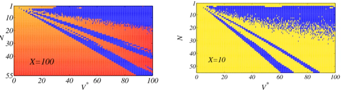
The procedure outlined in the previous section allows us to numerically construct an orbit of a single protocell. Hence we are in a position to analyze the sequence of successive division times (see top left panel of Fig. 3) and determine whether the associated behavior is regular or not. Fixing all the quantities but the ones of Eq. 5, one can construct a State Function as follows. For several values of ¯X and for each couple (N, V∗_{) defined over a large grid,}

(7)

orbit. If the latter is regular we assign to the State Function the value of the asymptotic division time, otherwise we set the corresponding case to a negative value (chosen to avoid possible superposition with the regular cases, the latter being characterized by positive division times). In Fig. 4 we report the State Functions obtained for different values of ¯X, in a typical setting. Some key qualitative features are always detected: domains of parameters (N, V∗_{) corresponding to regular and irregular behaviors coexist, being particularly well mixed}

in correspondence of specific zones. This peculiar pattern is of paramount importance and intrinsically relates to the speciation mechanism.

1 10 20 30 40 55 0 20 40 60 80 100 N V* X=100 0 20 40 60 80 100 1 10 20 30 40 50 V* N X=10

Fig. 4 – State Function. On the left: the State Function for ¯X = 100.0. On the right: the case relative to ¯X = 10.0.

Once several State Functions are stored, we can eventually simulate an open–ended Dar-winian evolution, monitoring the dynamical response of a population under the pressure of the sourrounding environment. To this end we introduce a mutation mechanism that is sup-posed to act on the double–stranded template length. In particular, we postulate that at each division (and halving) step, extra monomers are added or removed to the offsprings, according to a pre-assigned probability. Our simulations have been performed assuming a 2% mutation probability per monomer.

We then proceed as follows. For each protocell we set the template parameters. With respect to the first generation, M0(typically few units) protocells are created with an

associ-ated genoma, which follows an initial distribution. Typically, one may assume the very same genoma for all initial protocells. Consequently, the population is successfully represented by a unique vector with M0entries: each component containing the individual genoma parameters.

The initial population is supposed to live in an environment with available food, typically ¯

X = 100.0. For each protocell, we then extract from the State Function map the correspond-ing division time, if any, otherwise terminate the units that are associated to non–periodic behaviors (for a more complete discussion on the validity of this evolutionary assumption please refer to [1], [3], and [5]). The remaining protocells divide and produce two off-springs each, whose genoma can be different from the one of the mother, because of the mutation mechanism. Hence, the new population is described by a vector of length M1, of

size 2Nregular− Nirregular, Nregular and Nirregular labelling respectively the number of

reg-ular and irregreg-ular elements at the division. If the size of the population increases, then the available food for each protocell is decreased, and the next generation will be “governed”by another State Function panel (previously computed) which refers to the new food condition.

(8)

REFERENCES

[1] Carletti T and D. Fanelli, submitted to Europhys. Lett., (2006).

[2] G´anti T._{, Chemoton Theory: I) Theory of Fluid Machineries and II) Theory of Living Systems,} edited by Paul G. Mezey (Kluwer Academic/Plenum Publishers, New York) 2003.

[3] Carletti T., Stability, mutations and evolution in a population of Chemotons, submitted to J. Theor. Biol.,(2006).

[4] Matlab, The language of technical computing,http://www.mathwork.com,(2006).

[5] Carletti T. and D. Fanelli, Accepted paper BIOMAT2006 International Symposium, Novem-ber(2006) .