A Systematic Approach to Reliability Assessment of DC-DC Power Electronic Converters

(1)

HAL Id: tel-02302571

https://hal.archives-ouvertes.fr/tel-02302571v2

Submitted on 6 Feb 2020

HAL is a multi-disciplinary open access archive for the deposit and dissemination of sci-entific research documents, whether they are pub-lished or not. The documents may come from teaching and research institutions in France or abroad, or from public or private research centers.

L’archive ouverte pluridisciplinaire HAL, est destinée au dépôt et à la diffusion de documents scientifiques de niveau recherche, publiés ou non, émanant des établissements d’enseignement et de recherche français ou étrangers, des laboratoires publics ou privés.

DC-DC Power Electronic Converters

Vahid Samavatian

To cite this version:

Vahid Samavatian. A Systematic Approach to Reliability Assessment of DC-DC Power Electronic Converters. Electric power. Université Grenoble Alpes; University of Teheran, 2019. English. �NNT : 2019GREAT028�. �tel-02302571v2�

(2)

Pour obtenir le grade de

DOCTEUR DE LA COMMUNAUTE UNIVERSITE GRENOBLE ALPES

préparée dans le cadre d’une cotutelle entre la Communauté

Université Grenoble Alpes et l’Université de Téhéran

Spécialité : GENIE ELECTRIQUE

Arrêté ministériel : 25 mai 2016 Présentée par

Vahid SAMAVATIAN

Thèse dirigée par Hossein IMAN-EINI et Yvan AVENAS

préparée au sein des Laboratoires Power Electronics and Energy

systems et Grenoble Génie Electrique

dans les Écoles Doctorales School of Electrical and Computer

Engineering et Electronique, Electrotechnique, Automatique, Traitement du Signal (EEATS)

A Systematic Approach to

Reliability Assessment of DC-DC

Power Electronic Converters

Thèse soutenue publiquement le 27 mai 2019, devant le jury composé de :

M. Mahmud Fotuhi FIRUZABAD

Professor, Sharif University of Technology (Iran), Président

M. Farrokh AMINAFAR

Associate Professor, University of Tehran (Iran), Examinateur

M. Amir abbas SHAYGANI AKMAL

Assistant Professor, University of Tehran (Iran), Examinateur

M. Eric WOIRGARD

Professeur, Université de Bordeaux (France), Rapporteur

M. Laurent DUPONT

Chargé de recherche, IFSTTAR, Versailles (France), Examinateur

M. Jean-Luc SCHANEN

Professeur, Grenoble INP (France), Examinateur

Invités :

M. Hossein IMANEINI

Associate Professor, University of Tehran (Iran), Directeur de thèse

M. Yvan AVENAS

(3)

(4)

To my parents and my kind wife for their continuous

support and encouragement.

(5)

(6)

V | P a g e

Acknowledgements

Firstly, I would like to express my sincere gratitude to my advisors Dr.

Imaneini and Dr. Avenas for the continuous support of my Ph.D study and

related research, for their patience, motivation, and immense knowledge.

Their guidance helped me in all the time of research and writing of this

thesis.

Besides my advisors, I would like to thank the rest of my thesis committee:

Prof. Fotuhi Firuzabad, Prof. Bathaee, Prof. Woirgard, Prof. Schanen, Dr.

Dupont, Dr. Aminifar, Dr. Shaygani Akmal, for their insightful comments

and encouragement, but also for the hard questions which incented me to

widen my research from various perspectives.

My sincere thanks also goes to my brother, Majid, for enlightening me the

first glance of research and also his firm supporting during this research.

I am thankful to my colleagues Mr. Alexis Derbey, Mr. Benoit Sarrazin and

Mr. Florian Dumas who provided expertise that greatly assisted the

experimental aspect of our research.

I thank my fellow labmates in for the stimulating discussions, for the

sleepless nights we were working together before deadlines, and for all the

fun we have had in the last four years.

Last but not the least, I must express my very profound gratitude to my

parents and to my spouse for providing me with unfailing support and

continuous encouragement throughout my years of study, through the

process of researching and writing this thesis and my life in general. This

accomplishment would not have been possible without them. Thank you.

(7)

(8)

VII | P a g e

List of Figures

Fig. 1-1. Failure mode, mechanisms and effect analysis physics of failure reliability

assessment method ... 14

Fig. 1-2. Distribution of failure rates and their associated downtime in various part of wind turbine [40]. ... 17

Fig. 1-3. Reliability curves as a function of time for different scenarios [108]. ... 19

Fig. 1-4. Bathtub curve of failure rate [29]. ... 19

Fig. 1-5. (a) Effect of RDS-on variation of the MOSFET on the reliability of the converter. (b) Effect of capacitance C and ESR variations on the reliability of the converter [29]. ... 20

Fig. 1-6. (a) N-phase, interleaved boost converter model. (b) State-transition diagram of three-phase converter [27]. ... 21

Fig. 1-7. Flowchart to predict lifetime of power semiconductor in the operation mode [118]. ... 22

Fig. 1-8. Failure and stress distribution in power electronic components [40]. ... 24

Fig. 1-9. Abundance of power electronic semiconductors utilization [91]. ... 25

Fig. 1-10. Failure cost distribution [91]. ... 26

Fig. 1-11. Methods to improve reliability [91]. ... 26

Fig. 1-12. Correlation between various sectors and fragile components [91]. ... 27

Fig. 1-13. Correlation between various sectors and failure/cost ratio. [91]. ... 27

Fig. 1-14. Correlation between fragile components and failure/cost ratio [91]. .... 28

Fig. 1-15. Simpliﬁed IGBT device structure: a) equivalent circuit, b) PT, c) NPT, and d) TGFS [133]. ... 30

Fig. 1-16. Structure of sample discrete power devices ... 31

Fig. 1-17. Typical stress-strain (σ-ε) curve for a material. ... 32

Fig. 1-18. Damaged bonding wire. a) Cracked bonding wire full scale cross section [133], b) zoomed-in scale of (a) [133], c) foot crack [165], d) heel crack [165], e) fracture [165], f) lift off [165]. ... 37

Fig. 1-19. Damaged aluminum metallization. a) New device, b) Aged device [165, 39]. ... 37

Fig. 1-20. Solder joint. a) New device, b) Aged device [170]. ... 38

Fig. 1-21. On-state voltage drop measurement during aging test. a) PT, b) NPT, c) TGFS [134]. ... 39

Fig. 1-22. Competing physical phenomena responsible for the Vce, on variation in IGBT [134]. ... 40

Fig. 1-23. Generic variations in on-state voltage during IGBT aging. ... 41

Fig. 1-24. Strain-stress graph. (a) Typical, (b) Temperature-dependent curve of solder based on [177]. ... 43

Fig. 1-25. Coupled creep-fatigue lifetime estimation model. ... 44

(13)

XII | P a g e

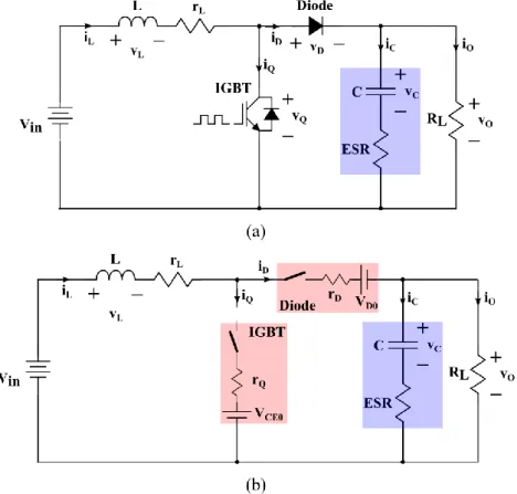
Fig. 2-2. DC-DC boost converter with parasitic components, (a) converter schematic,

(b) equivalent circuit... 54

Fig. 2-3. DC-DC boost converter key waveforms considering parasitic components. ... 55

Fig. 2-4. DC-DC boost converter with parasitic components, (a) on-state, (b) off-state equivalent circuits. ... 56

Fig. 2-5. Duty cycle command and resulted switching function. ... 58

Fig. 2-6. (a) Transient of capacitor voltage, (b) Steady state of capacitor voltage ... 63

Fig. 2-7. (a) Transient of Inductor current, (b) Steady state of Inductor current .... 63

Fig.2-8. I-V characteristics of IGBT and power diode (a) Collector-emitter voltage at 20℃, (b) Collector-emitter voltage at 175℃, (c) Diode forward voltage [213]. ... 65

Fig. 2-9. IGBT chopper driving an inductive load [214] ... 66

Fig. 2-10. Iterative algorithm for power loss calculation [215]... 68

Fig. 2-11. Thermal equivalent circuit model ... 69

Fig. 2-12. Physical configuration of IGBT and Diode. ... 71

Fig. 2-13. Assembly of chips on the heat sink ... 72

Fig. 2-14. Interested plate-fin heat sink ... 74

Fig. 2-15. Type of fluid flow [216] ... 74

Fig. 2-16. Plate-fin heat sink dimensions ... 76

Fig. 2.17. Equivalent thermal circuit of heat sink according to the various heat transfer mechanisms ... 77

Fig. 2.18. Temperature dependencies of a) heat transfer coefficients and b) heat sink thermal resistance... 78

Fig. 2. 19. Thermal model. (a) Foster model, (b) Cauer model. ... 80

Fig. 2-20. Process of thermal impedance extraction... 81

Fig. 2. 21. Thermal impedences of complete thermal model ... 82

Fig. 2. 22. 4-layer Foster thermal model expressing thermal impedances ... 83

Fig. 2. 23. Curve fitted of thermal impedances, a) ZIGBT, b) ZDiode, c) ZIGBT-Diode, d) ZDiode-IGBT. ... 84

Fig. 3-1. Thermo-sensitive electrical parameter test... 86

Fig. 3-2 TSEP voltages of a) IGBT and b) diode under 22.5mA low bias current ... 87

Fig. 3-3. Devices under test. a) Schematic circuit of IGBTs and diodes under test, b) mounted DUTs on cold plate ... 90

Fig. 3-4. Global thermal resistance. ... 91

Fig. 3-5. Implemented test bench for power cycling and thermal cycling accelerated aging tests. ... 91

Fig. 3-6. High current generator. a) schematic, b) switching pattern. ... 92

Fig. 3-7. Aging monitoring process. ... 93

Fig. 3-8. Collector-emitter Voltage during measuring period measured by 6-channel data acquisition (HBM-Gen3i_{) ... 94}

(14)

XIII | P a g e

Fig. 3-9. Number of cycles to failure of a) IGBT and b) diode exposed to APC. ... 96

Fig. 3-10. Deterioration trends of power semiconductors against various thermal cycles. a) IGBT, b) diode... 97

Fig. 3-11. Thermal cycling profile ... 98

Fig. 3-12. Parameters drifting during aging. ... 99

Fig. 3-13. Geometry of creep specimen...100

Fig. 3-14. Thermal and Electrical reliability correlations in a converter. ...100

Fig. 3-15. Conventional DC-DC boost converter equipped with auxiliary circuits. a) Schematic, b) switching pattern ...102

Fig. 3-16 Test bench of customized DC-DC boost converter ...103

Fig. 3-17. Main switching cell of the considered DC-DC boost converter ...103

Fig. 3-18. Gate driver circuit. ...104

Fig. 3-19. Schematic circuit of a) voltage clamping circuit and b) low bias current source circuit. ...105

Fig. 3-20. SEM microscopic image of solder joint, a) new device, b) aged device under APC test, c) aged device under ATC test. ...106

Fig. 3-21. 3D X-ray tomography of solder joint, a) new device, b) aged device under APC test, c) aged device under ATC test. ...106

Fig. 4-1. Time domain data versus cycle-counting domain ...110

Fig.4-2. Time domain data and its corresponding stress-strain hysteresis loop ...111

Fig. 4-3. Four-point thermal full cycle. ...113

Fig. 4-4. Flowchart of newly proposed online time-temperature-dependent creep-fatigue Rainflow counting algorithm ...115

Fig. 4-5. Sample load cycles. (a) Thermal cycles, (b) thermal cycles after creep and extremum checks ...118

Fig. 5-1. Conventional reliability assessment of critical components of power electronic systems. ...122

Fig. 5-2. A conventional DC-DC boost power converter ...124

Fig. 5-3. Mission profile, HEV speed based on WLTP-class3. ...125

Fig. 5-4. Junction temperature profiles. ...125

Fig. 5-5. Sorted junction temperature of IGBT and power diode for (a) fatigue and (b) creep lifetime models. ...126

Fig. 5-6. Frequency of damages in IGBT and diode. ...128

Fig. 5-7. Reliability function of IGBT and diode damages during one driving cycle ...128

Fig. 5.8. Reliability function of power capacitor in terms of hour ...128

Fig. 5.9. Reliability function of global multi component system, power capacitor, IGBT and power diode ...129

Fig. 5-10. A conventional DC-DC boost power converter. ...130

(15)

XIV | P a g e

case. ... 135

Fig. 5.13. Sorted junction temperature of IGBT and diode in the fully degraded case. ... 136

Fig. 5.14. Frequency of damages in IGBT and diode in fully degraded case. ... 137

Fig. 5.15. Reliability functions of IGBT and diode damages during one driving cycle in fully degraded case. ... 138

Fig. 5.16. Reliability function of global multi component system, power capacitor. ... 138

Fig. 5-17. Global flowchart of reliability assessment of n-component system ... 141

Fig. 5-18. Block diagram of the n-component system subjected to multiple failure processes. ... 142

Fig. 5-19. Degradation process of an effective item. ... 143

Fig. 5-20. Mapping matrix. a) Each state of effective items is allocated to a specific global system state, b) Three-item mapping matrix Hc where PϵΩ={M-1, M-2, …, 1}. ... 145

Fig. 5-21. Degradation processes of a) IGBT and b) power diode. ... 151

Fig. 5-22. Reliability functions of different states. ... 153

Fig. 5-23. Reliability functions. ... 153

Fig. A-1. Time-dependent duty cycle command and resulted switching function. 175 Fig. A-2. IGBT/diode layers... 178

Fig. A-3. Simulation results in ABAQUS environment based on analytic manipulations ... 178

Fig. B-1. Discrete Power semiconductor, a) structure, b) meshed model. ... 179

Fig. B-2. Accumulated strain, strain energy and stress distributions in the solder joint. ... 180

Fig. B-3. Accumulated creep strain in solder joint. ... 181

(16)

XV | P a g e

List of Tables

Table 1-1. A quantitative and qualitative comparison among five well-known

reliability handbooks ... 11

Table 1-2. Mission profiles [42] ... 13

Table 1-3. Example of Power Semiconductor failure mechanisms [43] ... 13

Table 1-4. Overview of failure modes, critical failure mechanisms and critical stressors [93] ... 48

Table. 2-1. Comparison of different approaches ... 58

Table 2-2. Working Conditions and Parameters Values ... 63

Table 2-3 Heat sink Dimensions and Thermal Parameters Values ... 78

Table 2-4. Parameters of Foster model of Thermal impedances according to equations (2-59) and (2-60) ... 82

Table 3-1. IGBT cycles to failure for power cycling accelerated tests ... 95

Table 3-2. Diode cycles to failure for power cycling accelerated tests ... 95

Table 3-3. Junction temperature of IGBT and diode ...105

Table 4.1. True table of algorithm ...119

Table 5-1Working Conditions and Parameters Values ...124

Table A-1. Rules of converting state-space model to TIMF ...176

Table A-2. Material general and thermal properties [211], [216], [219] ...177

(17)

(18)

XVII | P a g e

Abbreviations

AERs Alternative Energy Resources Al EM Aluminum Electromigration Al SM Aluminum Stress Migration Al-Caps Aluminum Electrolytic Capacitors APC Accelerated Power Cycling

ATC Accelerated Thermal Cycling BJT Bipolar Junction Transistor

CCM Continuous Conduction Mode

CTE Coefficient Of Thermal Expansion Cu EM Copper Electromigration

Cu SM Copper Stress Migration

DBC Direct Bonded Copper

DCM Discontinuous Conduction Mode DFR Design For Reliability

DUT Device Under Test

EOP Electrical Operating Point ESR Equivalent Series Resistance

FC Fuel Cell

FEA Finite Element Analysis FEM Finite Element Method FEoL Front End Of Line FFT Fast Fourier Transform

FMMEA Failure Modes, Mechanisms And Effect Analysis FSR Fourier Series Representation

GSSA Generalized State Space Averaging HEV Hybrid Electric Vehicle

i-EOP Interval Electrical Operating Point IGBT Insulated Gate Bipolar Transistors

inf Infimum

i-TOP Interval Thermal Operating Point i-ULE Interval Useful Lifetime Estimation

JEDEC Joint Electron Devices Engineering Council KBM Krylov-Bogoliubov-Mitropolsky

KCL Kirshohf Current Law

KTL Kirshoff Thermal Law

KVL Kirshohf Voltage Law

LTI Linear Time Invariant LTV Linear Time Varying

(19)

XVIII | P a g e

MPPF-Caps Metallized Polypropylene Film Capacitors

NPT Non-Punch Through

PCB Printed Circuit Board

PoF Physics-Of-Failure

PT Punch Through

PV Photovoltaic

PWM Pulse Width Modulation

RADC Rome Air Development Centre RBD Reliability Block Diagram

SAC Sn-Ag-Cu Based Solder

SAE Society Of Automotive Engineers SEM Scanning Electron Microscope SSA State Space Averaging

TDDB Time-Dependent Dielectric Breakdown TGFS Trench Gate ﬁeld Stop

TIMF Time Invariant Multi Frequency TMMC Time Mode Miller Compensation TOP Thermal Operating Point

TSEP Thermo Sensitive Electrical Parameter UGFs Universal Generating Functions

ULE Useful Lifetime Estimation

(20)

XIX | P a g e

Notations

{A1, A2, B1, B2,} System matrices

~N(μ,σ2₎ _{Normal distribution with mean value of μ and variance of σ}2 ~W(η,β) Weibull distribution of η scale factor and β shape factor < X(t)>T Average value of X on switching period

∆Theatsink Heat sink temperature swing

A Coefficient of Coffin-Manson-Arrhenius lifetime model

Af Front area of HEV

Afin Total fin area

Aplate Plates total area

Arad Total area of radiation heat transfering BS Battery share of power transferring

BVCES Breakdown voltage

C Capacitance

c Time varying trigonometric vector

CD Aerodynamic drag coefficient

chs, shs, dhs, hhs,

whs, ths, ℓhs Dimensions of heat sink (Fig. 2-16) Cies/Coes/Cres Input/output/reverse capacitances

Cσ Parasitic capacitance

D Total damage (chapter 1 and 4, 5)

D Duty Cycle (chapter 2)

d Duty cycle state variable

d(t) Duty cycle command

DCap Damage function of capacitor DDiode Damage function of diode

DIGBT Damage function of IGBT

Dj(t) Degradation process of jth_{ineffective component}

E[T] Mean time to failure

Ea Activation energy

EonD, EoffD Diode switching energy losses EonQ, EoffQ IGBT switching energy losses

F Failure state

fr Rolling resistance coefficient

fSW Switching frequency

g Gravity

Gi Threshold value of ith_{effective component} h Convective heat transfer coefficient

Hc Mapping matrix

(21)

XX | P a g e

i Inductor voltage state variables

I Unit matrix

i- ΔTj Interval temperature swing

I0(.), I1(.) The first and the second terms of Modified Bessel function of the first kind

iC(t) Capacitor current

ICrms RMS current of Capacitor

id(t) Diode current

IDav Diode average current

IDrms Diode effective current

IDUT Current of DUT

Ii Input average current

ii(t) Converter input current

IL Inductor average current

iL(t) Inductor current

ILrms RMS current of Inductor Imeas Low bias measuring current io(t) Converter output current

IP Power current

iQ(t) IGBT current

IQav IGBT average current

IQrms IGBT effective current

i-Tj Interval junction temperature

K Coefficient of thermal resistance variation (equation (3-4))

k Total number of effective items

k0(.), k1(.) The first and the second terms of Modified Bessel function of the second kind

kair` Air conductivity

KB Boltzmann’s constant (8.62×10−5_ev/K) khs Heat sink thermal conductivity

ki Integral coefficient of PI controller

KID Diode current dependency on switching energy losses KIQ IGBT current dependency on switching energy losses kp Proportional coefficient of PI controller

KVD Diode voltage dependency on switching energy losses KVQ IGBT voltage dependency on switching energy losses

L Inductance

ℓ Total number of ineffective items

L and L0 Useful lifetimes under the use condition and testing condition

(22)

XXI | P a g e

Lσ Stray inductance

M Mass of the vehicle (Mission Profile)

M Global system degradation states (Multistate degraded system)

MI Output/input converter current ratio

Mi Degradation states of ith_{effective component} Mv Output/input converter voltage ratio

n Number of distinct cycles which power semiconductors are subjected to in Palmgren–Miner’s rule

n Voltage stress exponent in capacitor lifetime model

N Order of Fourier series

NF Number of cycles to failure in Coffin-Manson-Arrhenius lifetime model

NFi Number of cycles to failure of the ith particular cycle in Palmgren–Miner’s rule

nfin Number of fins

Ni Number of the ith_{particular cycle in Palmgren–Miner’s rule}

Nub Nusselt number

Nudev Nusselt number for developing region Nufd Nusselt number for fully developed region

Nui Ideal Nusselt number

Nulaminar Nusselt number of laminar region in the external plates Nuplate Nusselt number of plates

NuTurbulent Nusselt number of turbulent region in the external plates

P(.) Probability function

Paux Auxiliary equipment power

Pb Blocking power loss

Pconv Power converter

PCQ/CD IGBT/Diode conduction power loss

PDUT Power of DUT

PG Gate driving power loss

Pi Intermediate degradation state of ith_{effective component} PLossDiode Diode total power loss

PLossIGBT IGBT total power loss

PLossrC Capacitor internal power loss PLossrL Inductor internal power loss Pmax Pointer showing the length of Smax

Pmin Pointer showing the length of Smin

Po Output power

Pr Prandtl number

(23)

XXII | P a g e

q Switching function state variables

q(t) Switching function

qconv-fin Fins convective heat transfer qconv-plate Plate convective heat transfer qrad Radiation heat transfer

Qrr Reverse recovery charge of Diode

R Load resistance

ℝ Mapping range

R(t) Global system reliability function

R*eb Channel Reynolds number

Ra Rayleigh number

rC Capacitor resistance

rD Diode internal resistance

RDS-on Drain to Source on-state resistance

Reb Reynolds number

Rg Gas constant (8.314 jmol-_1.K-₁₎

Rg Gate driving resistance

RGlobal-series(t) Global reliability function of a series system Ri(t) ith_{subset of Global system reliability function} rL Inductor equivalent series resistance

rQ IGBT internal resistance

Rth(c-h) Thermal resistance from case to heat sink Rth(h-a) Thermal resistance from heat sink to ambient Rth(j-c)Diode Thermal resistance from Diode junction to case Rth(j-c)IGBT Thermal resistance from IGBT junction to case Rth-base Thermal resistance of heat sink base

Rth-fin Thermal resistance of fins

Rth-i ith _{thermal resistance in Foster thermal model} Rth-plate Equivalent thermal resistance of plates

Rth-rad-plate Thermal radiation resistance Rth-spread Spreading thermal resistance

Rx(t) Reliability function of xth item in a series system Sj Threshold value of jth_{ineffective component}

Smax Flexible buffer for maxima

Smin Flexible buffer for minima

T Input temperature vector

t Input time vector corresponding to T

T and T0 Temperature in Kelvin at use condition and test condition

Ta Ambient temperature

(24)

XXIII | P a g e

tc Creep time

TCErr Reverse recovery energy temperature coefficient TCEts Switching energy temperature coefficient

TCrD Diode resistance temperature coefficient TCrQ IGBT resistance temperature coefficient TCVD Diode voltage temperature coefficient TCVQ IGBT voltage temperature coefficient Temean Equivalent mean temperature

tFC Full cycle time

th High time in switching function

Th Heat sink temperature

TjDiode Diode junction temperature TjIGBT IGBT junction temperature Tjmax Maximum junction temperature Tjmin Minimum junction temperature

tℓ Low time in switching function

Tm Mean junction temperature

TS Switching period

u(t) Input vector

v Capacitor voltage state variables

V HEV speed

V and V0 Voltage at use condition and test condition

vc(t) Capacitor voltage

VCE Collector Emitter voltage

Vce,on On-state collector-emitter voltage

Vce,on- Nagetive component of on-state collector-emitter voltage Vce,on+ Positive component of on-state collector-emitter voltage VCE0 Collector-emitter saturation voltage

Vcontact Electrical contact resistance voltage drop in MOSFET-BJT model of IGBT

VD Diode voltage

VD0 Diode forward saturation voltage

VDUT Voltage of DUT

Vg Gate-Emitter voltage

VG-TH Gate threshold voltage

Vi Input average voltage

vi(t) Input voltage

vL(t) Inductor voltage

VMOS MOSFET region voltage drop in MOSFET-BJT model of IGBT VNB Drift region voltage drop in MOSFET-BJT model of IGBT

(25)

XXIV | P a g e

Von On-state voltage of the power semiconductors Vpn p+_-n-_{junction voltage in MOSFET-BJT model of IGBT}

Vref Reference voltage

WMi Threshold value of state M in ith_component

x State variables (in FSR representation)

x(t) State vector

x(t) Average state vector

X Minimum value of parameter X

X Maximum value of parameter X

x(t) FSR of x(t)

x0(t) Time dependent zero component of FSR of x(t) Xfully-degraded Fully degraded component

Xnew New component

xαn(t) nth_{even component of FSR of x(t)} xβn(t) nth_{odd component of FSR of x(t)}

Yi(t) Degradation processes of ith_{effective component} ZDiode Diode thermal impedance

ZDiode-IGBT Cross coupling thermal impedance of IGBT on diode

ZIGBT IGBT thermal impedance

ZIGBT-Diode Cross coupling thermal impedance of diode on IGBT

Zth Thermal impedance

α Exponent of Coffin-Manson-Arrhenius lifetime model

βair Air density

Γ Characteristics length

γ Ratio of total heat sources surface and the heat sink base area

δ Mass factor

ΔiL Inductor current ripple

Δt Creep dwelling time

ΔTj Junction temperature swing

ΔvC Capacitor voltage ripple εrad Emissivity of Heat sink

η Converter efficiency

ηfin Fin efficiency

ηt Total efficiency of transmission system and electric motor

λ Failure rate

λ(t) Time varying failure rate

νair Air viscosity

(26)

XXV | P a g e

σ Mechanical stress (Chapter 1)

Boltzmann constant (5.669×10-8_W/m2_k4_{) (Chapter 2)} τi ith _{thermal time constant in Foster thermal model} Φ Cumulative normal distribution function

Ω Derivative matrix of c (dc/dt=-c Ω)

Ω Modified Global system state space (Chapter 5)

Ωi ith effective component state space

ωS Angular switching frequency

(27)

(28)

Introduction

On a global scale, burning of fossil fuels for supplying power are causing irreparable damage to our environment and disturbing the ecological balance. It is not possible to continue in this way without there being dire consequences. Therefore, developing alternative energy resources and full and hybrid electric vehicles (HEV) seems to be essential. Renewable energies can make a real difference as a golden opportunity. Due to the uncertain inherent of renewable energy resources, power conditioners are required for supplying the demanded power. Researchers are pushing back the frontiers of knowledge of power converters every day. Harnessing of technology in all sort of creative ways for designing reliable power converters grasps the importance. New cutting-edge design of power converters is transforming our visions from narrow-minded design to the reliable design of power converters. Importance of reliability of power converters is a widespread belief for long-term investment and stimulating the investors.

Reliability of power electronic converters plays a central role in persuading the investors and general users since renewable energy resources and other related issues have the lion’s share in supplying power demands. We also take the view that reliability assessment of a power converter is contributing factor in its design. Keen interests have been paid to the reliability of the power electronic converters either in component-level or in system-level.

Among all the power electronic converters, DC-DC power converters make a meaningful contribution in transferring and smoothing electrical power. Abundance use of DC-DC power electronic converters is a compelling reason for its importance as a reliability point of view. Several frameworks have been established for reliability assessment of DC-DC power converters and also a heated debate has been sparked off for DC-DC power converters reliability evaluation. The new reliability discipline focusing on mathematical or physical reliability assessments have been widely applied to the power converters. However, each of them has their own pros and cons. Those who support the claim of mathematical reliability evaluation advocate that this method is capable of assessing system-level reliability. On the other sides, some researchers who have taken the position of physical reliability

(29)

2 | P a g e

assessment have laid emphasize on its capability of considering the failure mechanisms and mission profiles.

In mathematical approach (called also as structural approach), collected reliability data in the specified field has been utilized. Despite its wrong basic assumption, namely an exponential distribution of failures, reliability hand books have become the almost exclusive prediction method for the reliability of electronic systems. Mathematical approach is capable of assessing reliability either in a component- or in a system-level employing some stochastic processes. This means that if a power electronic converter can roughly-appropriate works under a local failure occurrence, the method is still able to assess the reliability. The weakness point of this kind of reliability assessment is the absence of mission profile consideration such as temperature cycles and operational cycles. In addition, degradation and wearing out of one component on itself and on the other critical components is not taken into account leading to much more optimistic reliability assessment.

Physical approach or physics-of-failure (PoF) based approach is based on the knowledge of failure mechanisms by which the considered components and systems are failing. This method requires the knowledge of deterministic sciences and probabilistic variation theories. Consideration of the mission profile including both environmental and operational factors is one of the notable points of physical reliability assessment leading to much more realistic reliability estimation of a component. In addition, the wearing out of a component is also taken into account. However, in addition to its high cost and being time consuming, the detriment of this method as well as mathematical approach is the lack of consideration of mutual and self-degradation effects on itself and each other. The weakest point of this method is that it is restricted to the only component-level or multi component-level reliability assessment. Although, this method can deal with the simple reliability constructions such as series, parallel and k-out-of-n systems (multi component-level), it is not suitable for reliability evaluation of redundant system such as interleaved power converters. Because in the redundant systems, by changing the configuration of the system, operating conditions of the power converter would be varied leading to different damage models.

Thesis objectives and contribution

Lack of consideration of the dependencies (self- and mutual degradation effects) of the power converter’s components in both approaches, lack of consideration of the mission profile in mathematical approach and inability of tackling system-level reliability evaluation in physical approach as well shape our thinking to provide a rationale to meet the above mentioned challenges. The thrust of our argument is to merge all the advantages of both approaches by developing a physical reliability assessment approach.

(30)

3 | P a g e

By time passing, it is clear that the degradation process of a component or a system might be accelerated owing to the aging. Accordingly, static reliability assessment has not been able to estimate the reliability of a system and some dynamic reliability assessments seem to be required. For mitigating the problems of system-level reliability assessment, consideration of self and mutual degradation effects (dependencies), degradation levels (states) and consideration of mission profile, a new method has to be put forward.

The objectives of this thesis are to integrate the pros of both mathematical and physical methods and also tackling their detriments. In the proposed method, mission profile of undertaken system has been considered and applied to a multistate degraded system. This approach tries to consider the dependencies between the power components by defining a finite number of states for the global system. In the other word, this method converts a dependent system to a multi-state independent system by discretizing the global system states to the specific state space. In each state of the global system, detached operating conditions are assumed. Accordingly, in addition to the aforementioned challenges, this method is capable of analyzing time-varying failure rate.

Thesis framework and limitations

Two different reliability assessment frameworks will be proposed in this thesis for tackling abovementioned detriments. The first one is interval reliability analysis. By using interval reliability analysis instead of an inaccurate value for reliability, one can find an interval for the reliability of power electronic converters. Degraded and new states of the global system (power electronic converters) both are considered in this approach. The second approach is multi state degraded reliability assessment and defining a finite number of states in the global system to consider dependencies. As a case study, a conventional DC-DC boost converter is taken into account as an interface between a battery bank and a motor driver in HEV. A customized 3000W 200V/400V setup was implemented for validating the effects of degradations (dependencies) in the power electronic systems. Based on the literature review, the two most critical components in the power electronic converters are power semiconductors and power capacitors. It has to be mentioned that the customized DC-DC boost converter consists of an IGBT and a power diode as power semiconductors.

Employing the customized conventional DC-DC boost converter, we were able to observe the effects of self- and mutual degradations of the components on each other. Accordingly, the first challenge, namely dependencies, has grasped the importance. For providing aged devices (power semiconductors), an accelerated thermal cycling (ATC) aging test was performed.

(31)

4 | P a g e

For validating the new frameworks, i.e. interval reliability assessment and multi state degraded system, some aging information was extracted from an accelerated power cycling (APC) aging test. Regarding to the time limitation, the main focus of aging have been zoomed on the power semiconductor aging tests and power capacitors’ data has been extracted from literature reviews.

Thesis organization

Chapter one deals with the literature review and fundamental theories of conventional approaches. In this chapter the failure mechanisms of the critical power components and their correlations in their lifetime models have been discussed. Chapter two expresses electrical, thermal and power loss modeling of DC-DC boost power converter. In this chapter, time invariant multi frequency (TIMF) modeling capable of evaluating states’ ripples has been investigated. Iterative power loss calculation is also expressed. The chapter is ending with the forced convection heat sink design and expressing a complete dynamic thermal modeling. While, chapter three deals with the experimental procedure and their results including thermo sensitive electrical parameter (TSEP) tests, customized DC-DC boost power converter, accelerated power cycling aging test, accelerated thermal cycling aging test, scanning electron microscope (SEM) and 3D X-ray tomography microscope, a newly proposed cycle counting algorithm capable of considering time-temperature mean value and creep-fatigue failure mechanism is launched in chapter four. Chapter five is expressing the reliability assessment of 3000W 200V/400V DC-DC boost power converter as an interface power conditioner in an HEV exposing to worldwide harmonized light vehicles test procedure (WLTP) driving cycle. The reliability assessment falls into three categories, namely conventional physical approach, interval reliability analysis and multi state degraded reliability assessment, in this chapter. Finally, a conclusion and summary is drawn in the last chapter.

(32)

1

Literature review

1-1 Introduction

There is undoubtedly no dispute in the importance and necessity of the reliability of an item. Small wonder, then, that general users lay emphasize on how reliable products they utilize. In addition, some organizations such as military systems and airline companies are fully aware of the costs of their unreliable products and try their bests to make their services as reliable as it is possible. Manufacturers have also dealt with their products’ reliability and done their bests to make their business profitable. They often push up a huge cost of failure under warranty period time. Although the costumers have accepted failure occurrence in their products, they are becoming highly sensitive to the failure in warranty time. Thus, manufacturers inevitably have to estimate the reliability of their products for the warranty period. The ability of well working (without occurring any failure) of a product/system/ equipment in the certain period of time is the raised question addressing with the aid of the science of probabilities and statistics. Therefore, a clear definition of reliability engineering is [1]:

“The probability that an item will perform a required function without failure under

stated conditions for a stated period of time.”

Reliability as a simple definition is the number of failures in a specific period of time. Generally, the objectives of reliability engineering are falling into the following categories [1], [2]:

1- To apply engineering and technical knowledge in order to avoid or to decline the probability or frequency of failures.

2- To identify and to mitigate the prime causes of failures that do occur whether or not some efforts have been made to remove them.

3- To determine some ways of relieving the failures that do occur providing that their causes have not been eradicated.

(33)

6 | P a g e

Hence, reliability assessment is said to be an inseparable part in engineering fields. However, considerable challenges have been also remained and have to be wrestled [3], [4].

An engineering product could fail owing to different reasons. The main reasons are as follows: inherently capability of product design, exposing to the overstressed working environment, product wearing out, uncertainty of product strength or uncertainty of applied load (strength-stress variation), time dependency of failure mechanism, errors owing to incorrect specifications and design. Failures have various causes and effects and there are also different concepts, perceptions and definitions for categorizing the events in the failure or not [1], [4].

Reliability history belonged to the much earlier time. However, the new reliability discipline focusing on one of the Rome Air Development Centre (RADC) objectives, namely “developing prediction methods for electronic components and systems”, launched in early 1960s [2]. Two launched approaches fell into two following categories:

1- Statistical approach (also called mathematical approach): in this method, collected reliability data in the specified field has been utilized. MIL-HDBK-217A is the first reliability prediction handbook published in December 1965 by the US Navy. It shed the light being well accepted by all designers of electronic systems, owing to its flexibility and ease of use. Despite its wrong basic assumption, namely an exponential distribution of failures [5], MIL-HDBK-217A became the almost exclusive prediction method for the reliability of electronic systems, and subsequently other sources of prediction methods gradually disappeared [6]. 2- Physic of failure approach (PoF and also called physical reliability): it is based on

the knowledge of failure mechanisms by which the considered components and systems are failing. This approach was firstly taken into account in Physics of Failure in Electronics symposium sponsored by the RADC and the IIT Research Institute (IITRI), in 1962. However, this symposium worked in the different name of International Reliability Physics Symposium (IRPS) which was the most influential scientific event in failure physics.

The two approaches seemed to be distinctive; system engineers were focused on the ‘statistical approach’ while component engineers working on PoF. However, both groups realized that two methods were complementary and attempted to unify the two approaches.

In 1974, the RADC as a promoter of PoF approach became responsible for providing the second version of MIL-HDBK-217, and of also its subsequent successive versions (C to F). In the latest versions, they tried to update the handbook by considering new advances in fabrication technology. However, more complex models were extracted which made the new models too complex, too costly and unrealistic [6]. In the 1980s,

(34)

7 | P a g e

a lot of manufacturers of electronic systems had tried to develop specific prediction methods for reliability such as proposed models for automotive electronics by the Society of Automotive Engineers (SAE) Reliability Standards Committee and for the telecommunication industry (Bellcore reliability-prediction standards).

1-1-1 Statistical method

In this approach, mathematical models based on the experimental and/or test data has been used for reliability assessment of an item, especially, electronic components such as different types of transistors, capacitors, etc. These models and data as well could be found in different reliability handbooks. Reliability assessment based on the reliability handbooks has two features as follows [7], [8]:

1- Failure rates are sorted and listed in the “Failure Rate Table” based on the components type.

2- Correction factors are being prepared for modifying the failure rates in the different conditions.

Accordingly, statistical method has tried to estimate the reliability of a specified item (here it can be considered as an electronic component) utilizing constant failure rates during their performances. Heretofore, a huge number of reliability handbooks have been provided by various organizations (but mostly military organizations) in order to evaluate and estimate reliability of electronic components [7]–[11]. Some of them are explained here as a snapshot.

1-1-1-1 MIL-HDBK217 reliability handbook

MIL-HDBK217 is one of the most important reliability hand books and has been extensively applied in electronic equipment and components reliability assessment. It has been published in 1965 by US navy [2]. It comprised a significant number of electrical components and devices and thus, its importance and ease of use being grasped by various military and commercial organizations [12]–[15]. Nevertheless, its proceeding versions have been published in the different periods of time regarding ever-increasing new electronic components production. The latest version was published in1995 and never has been updated yet. However, it has to be mentioned that there are still substantial number of studies employing such reliability models based on MIL-HDBK217 [15]–[17].

Two estimation models, namely part count and part stress, have been provided in MIL-HDBK217. Part count model is applied in the initial design phases in which the number of components and their quality levels are specified [7]. In this model, there is no detailed information about the components and stress level they are exposed to. Part stress model is based on the effects of mechanical, electrical and environmental stresses such as temperature and humidity on the failure rates. This model is used whenever the design has been roughly completed and the details of

(35)

8 | P a g e

applied stresses has been determined. Since much more information is in access, more precise estimation is achieved in comparison with part count model.

In this model, environmental coefficients indicates the environmental stresses on the components or equipment. Almost all of the environmental stresses have been considered in the latest version [7]. Part stress model, in the component level (but not in the system level), calculates the component failure rate of a component regarding to the applied environmental stresses. For instance, a component failure rate can be estimated as follows:

P b Q E A T V

        _(1-1)

where _bis the base failure rate extracted from experimental tests in an specified condition. Correction factors are including _T (temperature coefficient), _A

(application coefficient), _V (voltage stress coefficient), _Q (quality coefficient) and

E

 (environment coefficient). Equipment failure rate (at the system level) can be predicted using part count models as follows:





n EQUIP part i g _{Q i} i 1 N _   



  (1-2)

where _EQUIP is the equipment failure rate. _gand _Q are the general failure rate and quality coefficient for the ith_{component, respectively. Npart-i is the number of i}th component in the system and n is the total number of different components in the system.

MIL-HDBK-217 has provided a considerable database for many different types of parts including capacitors, switches, relays, magnetic devices, printed circuit board (PCB), etc. This reliability handbook prepares a uniform reliability assessment database without emphasizing on significant reliability experiences as a particular component [13], [14]. However, this reliability handbook does have limitations [7]. Assuming a constant failure rate for different components during their useful lifetimes is one of the main limitation this reliability handbook confronts to [3]. Field experiences show that the reliability estimation of either components or systems have been significantly optimistic. Furthermore, it does not reflect the temperature swing effects (or any other mission profile which are completely important to power electronics converter) leading to an inaccurate life estimation. Failure rate models and database of some components such as insulated gate bipolar transistors (IGBT) have not been included and thus the other switches have been considered instead.

1-1-1-2 IEC-TR-6238 reliability handbook

This reliability handbook was published in 2004 and aimed to assess the reliability of power electronic components and equipment [8]. Environmental and performance stresses have been also considered in power electronic components’

(36)

9 | P a g e

reliability assessment as it has been done in the MIL-HDBK-217. With regard to the application, level of effectiveness of these kinds of environmental stresses (mechanical, chemical, etc.) has been launched [18].

In addition to the above-mentioned parameters and coefficients, another parameter called “mission profile” parameter has been also seriously contemplated through reliability assessment in order to increase the accuracy of reliability estimation of power electronic components. In fact, mission profile reflects loading level of power electronic components (regarding to their application and the converter topology). For example, irradiation level is being identified during the year regarding the global irradiation map [19]. Hence, in the photovoltaic (PV) applications, the power which can be harvested from the sun irradiation and transferred to the grid utility via a PV inverter might be specified. Accordingly, one can calculate the electrical stresses (finally resulting to thermo-mechanical stresses in PV inverter components) during a year or any other specified period of time. This weakness (lack of considering mission profile) is evident in MIL-HDBK-217 reliability hand book. It generally means that the correction factors have only effects on the base failure rate of the component under specified conditions (stresses). For instance, πTis considered as a constant temperature coefficient assuming that the component is exposed to the specified stresses in MIL-HDBK-217 reliability handbook. Thus, it is not the case in the real applications in which the component confronts various stresses (mission profile). Furthermore, a much more reliability estimation is achieved regarding the consideration of failure sites e.g. package or chip (die) in this reliability handbook. For example, a mathematical model of power diode gives:





 

   





y i t i z 0.68 3 i 1 0 U i n _i B ₉ i 1 on off I EOS 2.75 10 T 10 / h            _ _{ }_ _ _ _  _{  }_ _{ }_ _ _ _ _ __ _               __ __         



_(1-3)

where πU is the utilization coefficient, λ0 the base failure rate of chip, (πt)i the ith temperature coefficient corresponded to the ith_{diode junction temperature in} mission profile, τi the ith_{working time of diode for the i}th_{diode junction temperature} in mission profile, τon(=Σyi=1 τi)and τoff the on and off working time of the diode, (πn)i the ith_{temperature cycling impact factor seen by the component package with} temperature cycle of T_i in the mission profile. _B, _I and _EOS are base failure rate

of packaging, utilization impact factor of diode and failure rate related to over stresses regarding the application, respectively.

Although, a considerable number of studies have made effort to assess the reliability of their systems by this reliability handbook [18]–[20], lack of consideration of

(37)

10 | P a g e

manufacturing technology and various types of power electronic devices result in inefficiency.

1-1-1-3 Other reliability handbooks

TELCORDIA-SR-332, BT-HRD-5, NTT, CNET, RDF93, RDF2000, SAE, SIMENS-SN-29500, 217-PLUS and FIDES are the other reliability references, especially employed in electronic and power electronic components’ reliability assessment, which have been developed their data based on the US army, transportation and telecommunication industries [21]–[24].

TELCORDIA-SR-332 is related to the telecommunication components and equipment and provides Bayesian analysis for reliability assessment. The principle of mathematical models of TELCORDIA-SR-332 is based on black box approach [24]. This part count approach defines steady state failure rate of equipment and based on the experimental data gives mathematical models for reliability assessment. Discussing other reliability references is beyond this study and hence interested readers are referred to [24], [25].

1-1-1-4 Comparison of reliability assessment based on the aforementioned reliability references

Table 1-1 indicates a quantitative and qualitative comparison among five well-known reliability handbooks, namely MIL-HDBK-217, TELCORDIA-SR-332, IEC-TR-62380, 217-PLUS and FIDES2004. Regarding this Table, one can find that 217-PLUS has paramount features in comparison with the other reliability references [26]. Numerous studies have been estimated reliability of power electronic converters by employing mathematical approach [20], [27]–[30]. These studies have been applied the above-mentioned reliability handbooks for calculating failure rates of different components and finally predicted system level reliability using stochastic processes (or other probabilistic methods). These probabilistic methods have been extensively used in reliability assessment and risk taking analysis in power electronic systems [3].

1-1-2 Physics of failure method

Despite that this approach has been extensively used in microelectronic reliability for the plenty of years, power electronic researchers have opened up a new issue in reliability assessment employing this method [31]–[39]. In power electronic systems, this method has been gained considerable interests among the researchers owing to the limitation of a systematic design for reliability (DFR) and optimistic reliability assessment by the other approaches [40].

(38)

11 | P a g e Table 1-1. A quantitative and qualitative comparison among five well-known reliability handbooks

Reliability references MIL-HDBK-217 IEC-TR-62380 TELCORDIA-SR-332 217-PLUS FIDES

Version F Edition 1 Issue 1 Edition 1 Issue A

Date of publication 1995 2004 2001 2006 2004 Failure rate Unit Failure in 106 hours Failure in 106 hours Failure in 109 hours Failure in 106_hours Failure in 109 hours

Software Yes Yes Yes Yes No

Default environmental

options

14 12 5 37 7

Component

model Multiplication Multiplication Multiplication Sum sum

Mission Profile No Yes No Yes Yes

Temperature

cycling No Yes No Yes Yes

Temperature rise in the component

Yes Yes Yes No Yes

Failure in

soldering No Yes No Yes Yes

Failure in off No No Yes Yes Yes

Bayesian

analysis No No No Yes No

On the contrary to the statistical method, PoF does not concentrate on a constant failure rate model of component and takes into account the mission profile in which the components are exposed to. Physics of failure is based on deterministic sciences (such as material and chemical sciences) and is able to assess the component reliability applying probabilistic and statistic sciences. Not only does this method assist in performance recognition and risk reduction in the design phase, but also models the failure root causes including fatigue, creep, fracture, corrosion, etc [41]. PoF based reliability assessment aims to find failure mechanisms and investigate the effects of mission profile on the critical failure mechanisms. This leads to transfer reliability analysis from component level to the failure mechanism and enhances it from reliability prediction to DFR [38].

In other words, physics of failure of electronic devices have been initially determined and then the failure root causes have been recognized. Based on the determined failure root causes (such as power cycling or temperature swing) and the mission profile (of the considered component) and employing reliability models, one can estimate component’s aging and useful lifetime regarding its mission profile.

(39)

12 | P a g e

In addition, by identifying the failure mechanisms and their corresponding root causes, one can use this data for condition monitoring of considered power electronic components. As an example, bonding wire lift off in a power semiconductor can decrease useful lifetime of the device. Thus, on-state voltage of power semiconductor (Von) can be utilized as a failure indicator providing that there is sufficient data about the relevance of this voltage to the aging of device [36].

1-1-2-1 Physics of failure terminology

In this section, some expressions which are commonly used in physic of failure method will be discussed.

 Mission profile (Load cycle): It is related to all operational or environmental (non-operational) conditions affecting the device. There exist numerous load cycles that can be individually or simultaneously applied. One can find some examples in Table 1-2.

 Failure mode: It is the effect by which a failure is observed including short circuit, open circuit, loss of gate control, parameter drift (RDS-on, ESR, C and …), etc. The permissive value of parameter drift is denoted through Failure criteria. In addition, one can use these parameter drifting as indicators. For example, 20% increase in RDS-on in power metal oxide field effect transistors (MOSFETs) is considered as the failure criterion.

 Failure mechanism: The physical, chemical, thermodynamic or any other processes which results in the failure. The failure mechanisms fall into two main categories, overstress and wear-out. Some examples are listed in Table 1-2 [42].

 Root cause (failure cause): A specific process, design and environmental factors that initiated the failure whose removal will eliminate failure. Some examples are listed in Table 1-3 [43].

 Failure site: A location in component which a specific failure occurs in it. Some examples are listed in Table 1-3.

 Failure criteria: Criteria or standards, with regard to applications, define or denote the failure boundaries. It is totally different from one component to the others and also from one failure mechanism to the other failure mechanisms. For example, a failure criterion is 100% increase of ESR in capacitor.

 Failure model: It relates to either deterministic or stochastic models (even both simultaneously) governing the failure mechanisms. Maybe, in the system level reliability assessment, newly established models are required.

 Damage indicator: It is in charge of indicating the degradation level of component required for maintenance or reliability evaluation. These damage indicators can be employed for condition monitoring. It is often used to stop the aging tests before failure using the Failure criteria.

(40)

13 | P a g e Table 1-2. Mission profiles [42]

Load Load conditions

Thermal steady state temperature, temperature swing (cycling), temperature gradient , _{temperature swing rate, thermal loss} Mechanical Pressure magnitude, pressure gradient, vibration, stress, strain

Chemical Humidity level, pollution, particles

Physical Radiation, magnetic interface, altitude

Electrical Current, voltage, power, frequency

Table 1-3. Example of Power Semiconductor failure mechanisms [43]

Failure Mechanism Failure Site Root Cause Failure Models

Fatigue

Die attach, wire bond/TAB, solder leads,

bond pads, traces, vias/PTHs, interfaces ΔT, Tmean, dT /dt, dwell time, J ΔV and ΔH Nonlinear power law (Coffin–Manson)

Corrosion Metallization M, ΔV , T Eyring (Howard)

Electro-migration Metallization T , J Eyring (Black)

Conductive filament

formation Between metallization M, ∇V Power law (Rudra)

Stress driven diffusion

voiding Metal traces S, T

Eyring (Okabayashi) Time-dependent

dielectric breakdown

Dielectric layers V, T Arrhenius (Fowler–

Nordheim) M: Moisture V: Voltage H: Humidity J: Current Density S: Stress T: Temperature

Failure modes, mechanisms and effect analysis (FMMEA) has been extensively used in PoF reliability assessment approaches as shown in Fig. 1-1 [32], [44], [45]. Firstly, the system and the components and the functions having to be analyzed are defined. Then, the potential failure mode is identified. Based on the mission profile (either operational or environmental) the potential failure causes are also identified. Next, the failure mechanisms and their associated failure models such as Coffin-Manson law are identified. Failure models are curve fitted by some accelerated aging tests. Finally, one can prioritize the most critical failure mechanism and begin PoF reliability assessment approach. Thus, identifying the critical failure mechanisms and their root causes as well is paramount of importance in reliability assessment based on the PoF algorithm.

1-1-3 Pros and cons of the two reliability assessment methods

As seen above, two distinct methods, namely mathematical approach and physics of failure based approach have been launched for years and years. However, none of them is capable of mitigating the challenges raising in this field.

On one side, as a mathematical reliability assessment point of view, this method is capable of assessing reliability either in a component- or in a system-level employing some stochastic processes. This means that if a system (power electronic

(41)

14 | P a g e

Fig. 1-1. Failure mode, mechanisms and effect analysis physics of failure reliability assessment method

converter as an example) can roughly-appropriate works under a local failure occurrence (one of the components fails during the normal working but the system is well working so far owing to the fault tolerance of system design), the method is still able to assess the reliability. Another weakness point of this kind of reliability assessment is absence of mission profile consideration such as temperature cycles and operational cycles. In other words, the failure rate (λ) is supposed to be constant during the systems’ performances.

DFR is one of the other important aspects in the reliability assessment which is playing a major role in the design of a reliable system. Since in the mathematical approach there is no consideration on root causes’ identification, thus there is no ability to enhance the reliability of the system in the design phase and the reliability assessment output is only and only a number. In addition, degradation and wearing out of one component on the other critical components is not taken into account leading to much more optimistic reliability assessment. Last but not least is the consideration of the components’ manufacturing technologies which is still lacking in the mathematical reliability assessment.

On the other side, consideration of the mission profile including both environmental and operational factors is one of the notable point of PoF based reliability