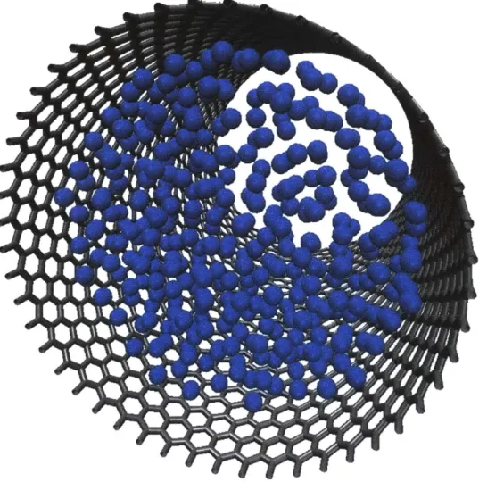
Atomistic engineering of fluid Structure at the fluid-solid interface

(line + symbol) for five aerosol components at 532 nm; (b) extinction Ångström exponents at 355–532 nm obtained from lidar observations and modeled by MERRA-2 for pure dust

convincing figures showing sections through the ditch (fig. 52) and questions relating to the nature and origin of the rubbish layer predating the use of this area as a military

On a remarqué que les données exposent des localités différentes et le cache de données unifié n’exploitent pas les localités exhibées par chaque type de

In fact, the Smirnov distribution of total amounts of time spent in the bulk af'ter n steps, equation (21), can provide us with such an expression for r (r, t if we make use of the

Whereas for submicellar solution, common non-ionic surfactants molecules usually undergo a diffu- sion limited adsorption, we showed that the adsorption of free surfactants from

Abstract : This study is devoted to the calculation, in transient mode, of the ultrasonic field emitted by a linear array and reflected from a fluid-fluid interface thanks to a

2shows the reflected pressure at a fixedheight h=2mm from the interface and at two different axis positions x=0mm and x=8mm.Differentpulses results, they corresponds to the direct

Thus the dependence of the dynamic contact angle on the three-phase line velocity appears to be frequency dependent above I Hz in our experiment. Moreover, the fact