HAL Id: hal-00302053
https://hal.archives-ouvertes.fr/hal-00302053
Submitted on 1 Jan 2001
HAL is a multi-disciplinary open access
archive for the deposit and dissemination of
sci-entific research documents, whether they are
pub-lished or not. The documents may come from
teaching and research institutions in France or
abroad, or from public or private research centers.
L’archive ouverte pluridisciplinaire HAL, est
destinée au dépôt et à la diffusion de documents
scientifiques de niveau recherche, publiés ou non,
émanant des établissements d’enseignement et de
recherche français ou étrangers, des laboratoires
publics ou privés.
ECMWF ensemble
C. Ziehmann
To cite this version:
C. Ziehmann. Skill prediction of local weather forecasts based on the ECMWF ensemble. Nonlinear
Processes in Geophysics, European Geosciences Union (EGU), 2001, 8 (6), pp.419-428. �hal-00302053�
Nonlinear Processes in Geophysics (2001) 8: 419–428
Nonlinear Processes
in Geophysics
c
European Geophysical Society 2001
Skill prediction of local weather forecasts based on the ECMWF
ensemble
C. Ziehmann
Nonlinear Dynamics Group, Institute of Physics, Potsdam University, Germany
Present address: Risk Management Solutions Ltd, 10 Eastcheap, London EC3M 1AJ, UK Received: 15 September 2000 – Accepted: 29 January 2001
Abstract. Ensemble Prediction has become an essential part
of numerical weather forecasting. In this paper we investi-gate the ability of ensemble forecasts to provide an a priori estimate of the expected forecast skill. Several quantities de-rived from the local ensemble distribution are investigated for a two year data set of European Centre for Medium-Range Weather Forecasts (ECMWF) temperature and wind speed ensemble forecasts at 30 German stations. The results indi-cate that the population of the ensemble mode provides use-ful information for the uncertainty in temperature forecasts. The ensemble entropy is a similar good measure. This is not true for the spread if it is simply calculated as the vari-ance of the ensemble members with respect to the ensemble mean. The number of clusters in the C regions is almost un-related to the local skill. For wind forecasts, the results are less promising.
1 Introduction
“No forecast is complete without a forecast of forecast skill!”
This slogan was introduced by Tennekes et al. (1987) dur-ing a workshop held at the ECMWF and has since then be-come a standard phrase in the context of ensemble predic-tion. By predicting the forecast skill we mean in this paper to provide a priori, i.e. together with each individual fore-cast, an individual estimate about the expected quality of this forecast. But while ensemble forecasting has developed into an integral part of numerical weather forecasting (Toth and Kalnay, 1993; Palmer et al., 1992; Houtekamer et al., 1996), skill forecasts are not yet always provided “operationally” by the national weather services. One exception is Meteo-France, issuing a 5 category confidence index (Atger, 2000). The results presented in this paper were achieved under a contract with the German weather service (DWD) with the aim to investigate the possibility of deriving skill forecasts
Correspondence to: C. Ziehmann
for weather parameters at German stations from the ECMWF ensemble.
Recently, the need for skill forecasts in its original mean-ing in terms of providmean-ing a forecast of the second moment of the distribution has been questioned as the forecast prob-lem could be set up completely probabilistically1. In many cases, however, a combination of a single forecast and its corresponding skill forecast may be still preferable, where the “single” forecast can be either a statistic based on the ensemble, such as the ensemble mean or a forecast which is independent of the ensemble. First, a joint forecast/skill fore-cast may be more rapidly understood and interpreted than probabilistic forecasts. Second, most numerical weather pre-diction (NWP) centers still run the ensemble forecasts with a model simpler than their best high resolution forecast model. Thus, the forecast could be based on the “best” model, while an estimate of the expected forecast skill could be derived from the ensemble. Hence, we focus our interest in this pa-per on the feasibility of first order skill forecasts based on ECMWF ensemble forecasts. In contrast to many other in-vestigations of this type, we analyze real weather forecasts at stations and not upper air fields; another difference is the verification method applied to quantify skill predictability.
2 Data
The results shown in this article are based on a 2 year data set between May 1997 and May 1999. It consists of the 50 ECMWF ensemble forecasts issued at 12:00 of temperature and wind speed2 for validation times 12:00 and 00:00 at 30 German stations. In addition, the corresponding observa-tions, the unperturbed control forecast, and the high
resolu-1See van den Dool (1992) and also related papers of Tennekes
(1992), Smith (1995, 1997), and Popper (1982) where the prob-lems of accountability, simplicity of the models, infinite regress, and higher order skill prediction are discussed.
2Precipitation and cloud-cover will be addressed in a follow up
0 0.5 1 1.5 2 2.5 3 3.5 4 4.5 -15 -10 -5 0 5 10 15 20 25 30 35 spread [C]
ensemble mean temperature [C]
spread versus forecast temperature 5 day forecasts Dresden
Jul 04 2000 0 2 4 6 8 10 12 14 -15 -10 -5 0 5 10 15 20 25 30 35 error [C]
ensemble mean temperature [C]
error versus forecast temperature 5 day forecasts Dresden
Jul 04 2000 0 2 4 6 8 10 12 14 1 2 3 4 error [C] spread [C]
error versus spread 5 day forecasts Dresden
Jul 04 2000
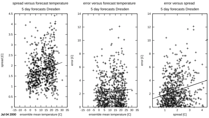
Fig. 1. Scatter plots of 5 day forecast errors of the high resolution forecast and ensemble spread (standard deviation with respect to the
ensemble mean). The left panel shows the spread as a function of the forecast ensemble mean temperature, the middle panel, the same for the error, and the right panel shows error versus spread. In all cases, a linear regression has been performed. Note the different scale of the ordinate in the left panel.
tion operational forecasts (T213 and T319) are used. Finally, the so-called Kalman filtered ensemble mean forecasts were also used in some cases in order to reduce the effect of sys-tematic model errors. Several changes in the Ensemble Pre-diction System (EPS) fall into this period: the introduction of evolved singular vectors (25 March 1998), the introduc-tion of a stochastic representaintroduc-tion of model uncertainty (21 October 1998), and the change in the number of vertical lay-ers from 31 to 40 (22 October 1999). The analysis, however, has not been performed separately for these sub-periods.
3 Quantifying skill predictability
Obviously, an ensemble which “spreads” out quickly in time indicates an uncertain forecast. In this paper, we investigate different definitions of the skill predictor “spread” and test their ability to stratify forecasts into certain and uncertain forecasts.
3.1 The traditional spread approach
Frequently, the variance of the ensemble with respect to a single valued forecast (for example, the control or the ensem-ble mean forecast) has been used as a measure of “spread”, which then has been related to the (absolute) error of this particular forecast. Not only variance-like measures but also correlation-type quantities are used for spread and skill (see, for example, Moore and Kleemann, 1998). The strength of
this relation is quantified either by the error-spread corre-lation (Barker, 1991; Whitaker and Loughe, 1997; Buizza, 1997; Ziehmann, 2000) or by contingency tables (Barkmei-jer et al., 1993; Houtekamer, 1992; Molteni et al., 1996; Whitaker and Loughe, 1997). Often, just scatter plots be-tween error and spread are shown, or they are processed into more informative conditional probability diagrams, as shown in Moore and Kleemann (1998). Common to all of these “traditional” approaches is that when calculating the spread, it is not taken into account whether the ensemble forecasts fall close to a climatologically mean value or to an extreme situation. This may turn out to be crucial, as will be shown below.
To give a first impression of this traditional approach, error and spread of 5 day temperature forecasts at the station Dres-den (station ID 10488) are shown in a scatter plot in the right panel of Fig. 1. In this case, the error of the high resolution forecast is shown together with the standard deviation of the ensemble members with respect to the ensemble mean. No stratification according to season has been made. A linear fit shows, as expected, a tendency for larger errors to occur at larger spread values. The error spread correlation coeffi-cient is about 0.3, thus the linear relation appears to be weak. For most spread values, almost the entire range of errors can occur. Only the smallest spread values seem to give rather certain indication for small errors.
Figure 2 displays the statistical relation between error and spread in these data as a function of forecast lead time, while
C. Ziehmann: Skill prediction of local weather forecasts based on the ECMWF ensemble 421 0 0.1 0.2 0.3 0.4 0.5 0.6 0.7 0.8 0.9 1 0 2 4 6 8 10 12 14 16 18 20 rel. frequency 12 h forecast steps SMALL spread 10488 t err1_spr1_3ec May 11 2000 p(small error) p(large error) 0 0.1 0.2 0.3 0.4 0.5 0.6 0.7 0.8 0.9 1 0 2 4 6 8 10 12 14 16 18 20 rel. frequency 12 h forecast steps MEDIUM spread 10488 t err1_spr1_3ec May 11 2000 p(small error) p(large error) 0 0.1 0.2 0.3 0.4 0.5 0.6 0.7 0.8 0.9 1 0 2 4 6 8 10 12 14 16 18 20 rel. frequency 12 h forecast steps LARGE spread 10488 t err1_spr1_3ec May 11 2000 p(small error) p(large error)
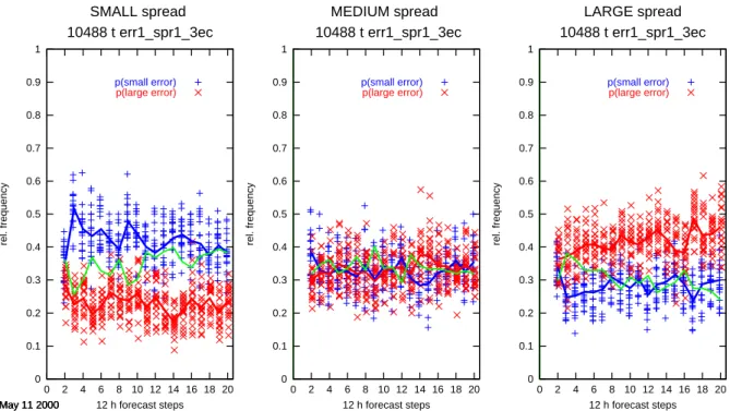
Fig. 2. Conditional relative frequencies for small (+, blue), large (×, red) and medium (green line) errors of the high resolution 2 m
temperature forecasts for the station at Dresden depending on the observed spread as a function of forecast lead time. The spread is the standard deviation with respect to the ensemble mean. The three panels show the results for the small, medium, and large spreads separately. Each of the symbols “+” and “×” corresponds to an independent evaluation of the data with a fit set of 500 cases drawn at random to define the threshold values of three equally likely classes of small, medium, and large spread and errors, respectively. The average of these repetitions is shown as a solid line. The data have not been stratified according to season.
-10 -5 0 5 10 15 20 25 30 1 2 3 4 5 6 7 8 9 10 11 12 temperature [C] month
10 - 90 % temperature percentiles for 0000h
-10 -5 0 5 10 15 20 25 30 1 2 3 4 5 6 7 8 9 10 11 12 temperature [C] month
10 - 90 % temperature percentiles for 1200h
Fig. 3. Boundaries of the ten equally likely temperature intervals at station Dresden (station ID 10488); on the left for the midnight
tempera-tures and on the right for the generally larger noon temperatempera-tures. Since no long temperature record was available when preparing this article, the climatology for each month was determined from the same 2 year data set of observations, leading to some wiggles in the nine 10% – 90% temperature percentiles.
also quantifying the confidence in this relation. In this case, the error of the high resolution forecast was contrasted with the standard deviation with respect to the ensemble mean. Each of the symbols “+” for small errors and “×” for large errors corresponds to an independent evaluation of the data with a fit set of 500 cases drawn at random to define the threshold values of three equally likely classes of small, medium, and large spread and errors, respectively. These thresholds are then applied to the independent test set of the remaining 200 cases to determine the relative frequencies of the occurrence of small, medium, and large errors when a small, medium, or large spread in the ensemble has been ob-served. The evaluation is repeated a couple of times, each time using new randomly determined fit and test sets, and the solid lines are the averages of these random samplings. Obviously, the definition of the spread used here does dis-criminate between cases with small and large errors. For ex-ample, when the spread is small (left panel), the chance of finding a small error is around 45% for the day 2 and 3 fore-casts, which is significantly larger than the 33% of finding a small error by chance. For medium spread, no conclusion can be drawn for the forecast error, and when the spread is large, again the frequencies for small and large errors differ from their random expectation values. Interestingly, the de-pendence of the forecast lead time appears to be weak and for the short term forecasts of 1 day the spread seems to provide almost no information.
The results above indicate that the ECMWF ensemble pro-vides information about the expected forecast error: here, even about the error of a forecast which is independent of the ensemble3 and thus, the ensemble appears to reflect the
at-mosphere’s inherent predictability. In the following, we will first show that quantifying skill predictability using spread and error as applied above may not be optimal and then we discuss an alternative approach originally suggested by Toth et al. (2000).
Both error and spread depend on the forecast state. One might expect that both quantities show larger values at the margins of the climatological distributions and smaller values when the forecast falls close to the climatological mean (Toth, 1991a,b). This is also the case in a maxi-mum simplification of a forecast/observation system with a red noise atmosphere and persistence forecasts (Fraedrich and Ziehmann-Schlumbohm, 1994); in this toy system, the amount of the error is directly proportional to the amount of the anomaly from the climatological mean. The left and middle panels of Fig. 1 show the observed spread and error values as a function of the forecast temperature and indeed suggest a behaviour with large values at the margins of the distribution which, in addition, seems to be superposed by a general but weak increase in error and spread with increasing temperature.
These results suggest that the projection of the
comprehen-3
Independent in the sense that the high resolution forecast is nei-ther a member of the ensemble nor a forecast derived from the en-semble.
sive information provided by the ensemble onto the scalar quantity spread is insufficient. The same spread value may indicate a large error if the forecast is near the climatologi-cal mean but a small error when the forecast is close to the margins of the distribution. Similarly, the same spread may indicate different forecast uncertainties for different times of the year. In the next section, we discuss an alternative. 3.2 Mode population as a predictor of forecast uncertainty The dependence of spread and error of the forecast state is taken into account by the method recently introduced by Toth et al. (2000) to quantify the ability of the ensemble to dis-tinguish between forecasts with small and large uncertainty. Both the ensemble forecast data and the observations are pro-jected into a given number of climatologically and equally probable intervals. Assuming a roughly Gaussian shaped tribution, the bins are wider towards the margins of the dis-tribution and narrower close to the mean. Figure 3 displays the nine class bounds which define ten equally likely 10%-intervals for temperature in Dresden for each month, with the generally lower midnight values on the left and the noon temperatures on the right.
Next, the number of ensemble members that fall into each interval is evaluated, as well as the interval corresponding to the observation. The mode of the ensemble is the most populous interval. The mode population is now used as the
skill predictor to stratity the forecasts according to their
ex-pected uncertainty. A high population reflects a certain or highly predictable forecast, while a small population indi-cates that there is only little agreement among the ensemble members, and thus a potentially poor forecast. When the en-semble mode agrees with the interval of the observation, the forecast has skill and is called a success, otherwise it has no skill. The skill predictor and “success” is thus a binary vari-able. The relative frequency of successful cases in the total sample is called the success rate. The success rate of a subset of forecasts, for example, for those forecasts with an espe-ciallly large mode population, is a conditional success rate. If these conditional success rates differ significantly from the average, the respective skill predictor is skillful.
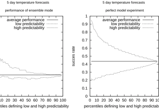
For 5 day forecasts, for example, the average success rate is about 28%, as shown by the horizontal solid line in the left panel of Fig. 4. The figure also shows conditional success rates for the highly predictable cases (with large mode pop-ulations) and the poorly predictable cases (with small mode populations), both depending on the thresholds used to de-fine high and low predictability. If one evaluates the success rate for those forecasts which belong to the top 10% with the largest mode populations, the success rate increases to about 45%. For the top 5% of mode populations, the success rate increases even more; however, one has to trade this increased success rate against the smaller number of cases in which one can issue such a “warning”. When the percentage ranges used to define unusual predictability approach 100%, the av-erage success rates are recovered. Figure 5 is directly related to Fig. 4 and shows the corresponding two threshold values in
C. Ziehmann: Skill prediction of local weather forecasts based on the ECMWF ensemble 423 0 0.1 0.2 0.3 0.4 0.5 0.6 0.7 0.8 0.9 1 0 10 20 30 40 50 60 70 80 90 100 succes rate
percentiles defining low and high predictability 5 day temperature forecasts
performance of ensemble mode average performance low predictability high predictability 0 0.1 0.2 0.3 0.4 0.5 0.6 0.7 0.8 0.9 1 0 10 20 30 40 50 60 70 80 90 100 succes rate
percentiles defining low and high predictability 5 day temperature forecasts
perfect model experiment average performance
low predictability high predictability
Fig. 4. Performance of the 5 day temperature forecasts at Dresden averaged over all cases (solid line) and those cases which are classified
as highly (dotted) or poorly (dashed) predictable. The results are presented as a function of the size of these classes. For example, the results shown at 10% use the 10% and 90% of the mode population to define the poorly (highly) predictable cases. The threshold values corresponding to these percentiles are shown in Fig. 6. The left panel shows results when verifying against the real observations in Dresden. The right panel displays a perfect model simulation of the same data, where the observation has been replaced by a randomly drawn ensemble member.
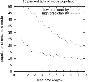
the mode population used for the stratification into high and poor predictability, as a function of the percentage of cases which are classified. For the 5 day forecasts and the top 10%, for example, the ensemble mode needs to exceed 35 ensem-ble members in order to be identified as a highly predictaensem-ble case, while it may contain at most 13 members for the 10% low predictable cases. Naturally, the population thresholds vary for a given percentage with forecast lead time as shown in Fig. 6. Now the two marginal percentage ranges used to define unusual predictability are fixed to 10%4. While for the 1 day forecasts, a top 10% predictability case requires that all 50 forecast members fall into one single interval, whereas on day 10 an ensemble mode with more than 18 members is al-ready considered as a highly predictable case, since in only 10% of the cases, the ensemble is still so tightly bound af-ter 10 days. Note that for a completely random forecast, one should expect 5 members per interval, on average.
When returning to the left panel of Fig. 4 the results for the poorly predictable cases appear to be not as pronounced as the cases where the ensemble mode has a large population. This suggests that it may be better to use non-symmetric per-centages when defining the thresholds for high and low pre-dictability and possibly issue a “poor prepre-dictability warning”
4
Note that Toth et al. (2000) define these thresholds such that 75% of all forecasts with medium predictability remain unclassi-fied.
only in the very few cases where the ensemble mode popu-lation is exceptionally small. The right-hand side of Fig. 4 shows the same analysis but under perfect model and perfect ensemble conditions, which have been simulated by draw-ing the “observation” at random from the ensemble (see also Molteni et al., 1996; Buizza, 1997). In this perfect case, the average success rate is notably increased and in partic-ular the poorly predictable cases are more distinguishable from the average than in the real world analysis. But even in the perfect model simulation, the figure is not symmetric with respect to the average success rate, and the information gain appears to be larger for large mode populations than for the small mode populations. This demonstrates once more (Molteni et al., 1996) that when spread is small, the forecast trajectory is constrained to be close to the observation; how-ever, when the spread is large, the forecast is not constrained to be far from the observation.
3.3 Other stratifications of ensemble forecasts
Before we compare the performance of the “normal spread” and the alternative approach using the ensemble mode popu-lated described in the previous section, we consider four ad-ditional scalar quantities which might also prove worthwhile for the stratification of ensemble forecasts into high and poor predictability. First, we introduce a bin spread, BS, which is similar to the standard spread but based on the ensemble
0 10 20 30 40 50 0 10 20 30 40 50 population threshold
percentile of mode population 5 day temperature forecasts Dresden
low predictability high predictability
Fig. 5. Mode population thresholds as a function of the percentage
ranges used to define poor and high predictability for 5 day fore-casts. The corresponding conditional success rates are shown in Fig. 4.
histogram with nbin intervals of varying width and their rel-ative frequencies fi, BS =P
nbin
i=1 fi|imode−i|, where imode
is the interval belonging to the mode. BS vanishes when all ensemble members fall into one bin. Thus, the smaller BS is, the smaller the uncertainty in the forecast. The entropy of the ensemble is S = −Pnbin
i=1 filog(fi) with filog(fi) = 0,
its limiting value, if fi = 0. It is also inversely oriented to
the mode population with a vanishing entropy when all en-semble members fall into one interval (then all intervals are empty and only fimode = 1) and it reaches the maximum
value Smax = log(nbins) when the ensemble distributes
uniformly into the nbin intervals. The number of non-zero bins N Z =Pnbin
i=1 H(fi), where H(x) = 1 for x > 0 and H(x) = 0 for x = 0, may also serve as an indicator for
skill predictability with a large number indicating reduced predictability. And finally, the number of clusters in the C region, as provided by the ECMWF, might give an indica-tion for forecast uncertainty with a large number of clusters indicating an uncertain forecast. Note that cluster informa-tion is based on the ECMWF ensemble as well, but on the geopotential for a region the size of Europe, on upper air data and on a fixed forecast time window. We have used the number of clusters in the C region (15◦W – 17.5◦E, 32.5◦– 57.5◦N, covering West and Central Europe), as provided op-erationally by the ECMWF. The ECMWF operational clus-tering is performed on the 51 ensemble forecasts, including the control of the 500 hPa geopotential fields in a time win-dow from 120 to 168 hours using a hierarchical cluster algo-rithm and a RMS similarity measure among the cluster mem-bers. For details, see the technical report (ECMWF).
All six scalar quantities are now used to stratify the ensem-ble forecasts and tested for their potential to indicate unusual
0 5 10 15 20 25 30 35 40 45 50 0 1 2 3 4 5 6 7 8 9 10
population of ensemble mode
lead time (days)
10 percent tails of mode population low predictability high predictability
Fig. 6. Mode population thresholds as a function of forecast lead
time when the top and bottom 10% of the ensemble mode popula-tion distribupopula-tion are used to classify poor and high predictability.
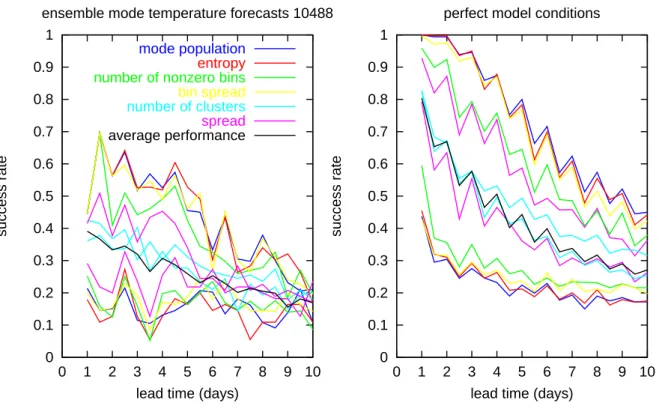
predictability. In each case, the 10% and 90% of these distri-butions are determined and used as thresholds for poor and high predictability. Then the respective conditional success rates have been determined, as well as the independent av-erage success rate. The results are shown in Fig. 7. Note that since we use 10 intervals, each covering 10%, a suc-cess rate of 10% is to be expected by chance. Again, the left panel of Fig. 7 displays the results for Dresden temperature forecasts and the perfect model simulations are shown on the right. The peaks in the curves at every second 12 hour in-terval result from forecasts for the two different verification times at 00:00 and 12:00. Note that the success rates of the real forecasts appear to be systematically larger for the mid-night verification time, while under perfect conditions, the midday temperatures show the larger success rates. Starting with the left panel, three quantities appear to be best suited for stratifying the ensembles forecasts: the mode population, the entropy, and the bin spread, since their conditional suc-cess rates differ most from the average sucsuc-cess rate. The number of non-zero bins provides only an intermediate re-sult, and the standard spread seems even less suited. Note that results might change for the normal spread if one would take the seasonal dependence into account; however, this has not been further addressed in this project. Almost no dis-crimination between certain and uncertain forecasts is made by means of the number of clusters. Thus, for local temper-ature skill forecasts, the local ensemble appears to be most relevant; however, alternative clusterings based on different algorithms (see, for example, Atger, 1998), variables, spatial domains, or time windows might provide more information about the local skill.
When using the three suitable skill predictors to stratify the ensemble forecasts, the gain in the success rate for the
C. Ziehmann: Skill prediction of local weather forecasts based on the ECMWF ensemble 425 0 0.1 0.2 0.3 0.4 0.5 0.6 0.7 0.8 0.9 1 0 1 2 3 4 5 6 7 8 9 10 success rate
lead time (days) perfect model conditions
0 0.1 0.2 0.3 0.4 0.5 0.6 0.7 0.8 0.9 1 0 1 2 3 4 5 6 7 8 9 10 success rate
lead time (days)
ensemble mode temperature forecasts 10488 mode population
entropy number of nonzero bins
bin spread
number of clusters spread
average performance
Fig. 7. Conditional success rates of the top 10% and bottom 10% predictable cases when classified using the 6 different “skill predictors”
with line types shown in the figure, as well as the average performance for temperature forecasts at the station Dresden. The right panel shows again, the perfect model simulation and hence, the potential improvement.
0 0.1 0.2 0.3 0.4 0.5 0.6 0.7 0.8 0.9 1 0 1 2 3 4 5 6 7 8 9 10 success rate
lead time (days) perfect model conditions
0 0.1 0.2 0.3 0.4 0.5 0.6 0.7 0.8 0.9 1 0 1 2 3 4 5 6 7 8 9 10 success rate
lead time (days)
wind forecasts Dresden biasfree mode population
entropy number of nonzero bins
bin spread
number of clusters spread
average performance
Fig. 8. Same as Fig. 7 but for wind speed forecasts at Dresden. In this case, each ensemble member has been corrected by the difference
highly predictable cases can be larger than 20%, compared to the average success rate. Alternatively formulated, the per-formance of the 10% highly predictable cases for lead times between 6 and 8 days compares to the average quality of 1 to 3 day forecasts, which is astonishing. The results for the en-semble mode population agree qualitatively very well with those reported by Toth et al. (2000), who contrast 500 hPa height ensemble mode forecasts with ensemble mode popu-lation. In their study, however, the conditional success rates for the highly predictable cases differ by as much as 35% from the average success rates which is likely due to the bet-ter performance, in general, of the 500 hPa forecasts com-pared to the surface variables.
Note that the forecasts have not been post-processed in this case and no calibration was necessary here. This was possi-ble since the temperature forecasts for the station at Dresden are “well behaved” and do not suffer from significant model errors. Other stations, for example, the Wendelstein (station ID 10980) at an elevation of 1832 m, show a large system-atic error and the skill forecasts are not nearly as good as for Dresden. But when correcting each ensemble member by the difference between the ensemble mean and a post-processed ensemble mean (a so-called Kalman filtered ensemble mean is operationally performed at DWD), skill forecasts also be-come feasible.
The results in the left panel of Fig. 7 are influenced to a large extent by model errors. The perfect model simulation results are shown in the right panel. Naturally, the overall results are better, but the relative differences between the 6 skill predictor remain more or less unchanged. Entropy, bin spread, and mode population appear to be best suited, with the mode population providing the absolute best results. This is to be expected under ideal conditions as the ensemble mode population indicates the likelihood of the verification falling into that bin, while entropy and bin spread approxi-mate this characteristic.
In another verification setup, these 6 scalar quantities de-rived from the ensemble have been used as indicators for the predictability of the high resolution model forecasts which are not directly linked to the ensemble. Also in this case, some of the 6 quantities provide useful information for the skill of this independent forecast. The success rates are only a little smaller and in this case, the entropy performs (marginally) better than all other skill predictors (figures not shown).
Next, we analyze another weather parameter at the same station. The results for 10 m wind speed are given in Fig. 8. Although each ensemble member has been corrected for the bias, the overall results, including the average success rate, are not as good as for temperature. This is consistent with the general result that wind speed belongs to those parame-ters which are quite difficult to predict (Balzer et al., 1998), as wind speed is very sensitive to local properties and the vertical stability of the atmosphere, both of which are not well represented in medium range forecast models. The best skill predictor cannot be uniquely identified, as is the case for temperature. The bin spread appears to be the best for most
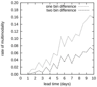
0.00 0.02 0.04 0.06 0.08 0.10 0.12 0.14 0.16 0.18 0.20 0 1 2 3 4 5 6 7 8 9 10 rate of multimodality
lead time (days) one bin difference
two bin difference
Fig. 9. Relative frequency of “multi-modality” of the temperature
ensemble forecasts at Dresden, when multi-modality is defined by finding a second, almost equally populated bin separated by at least two intermediate bins from the mode (long dashed). A weaker def-inition which requires only one intermediate bin leads to a larger fraction of multi-modal cases (short dashed).
but not all forecast lead times. The perfect model results on the right-hand side do not differ much from those for temper-ature and they show the same order for the skill predictors. These results also show that model errors are responsible for the poor results for wind speed, which cannot simply be re-duced by subtracting a constant value from each ensemble member. Thus, post-processing of the direct ensemble fore-casts at stations might be necessary as well as worthwhile, but this problem has not been systematically investigated in this study.
3.4 A closer look at the ensemble distributions
One might wonder why the bin spread, the entropy and the ensemble mode population perform similarly well, although the ensemble mode population seems to contain a smaller amount of information than the other two quantities, as it only requires the frequency in one single bin. Does this mean that in most cases, the ensemble is unimodal with no further peaks of similar height in the distribution? A simple test on multi-modality has been applied here. Whenever the second most populated bin was separated by at least 2 intervals from the ensemble mode and displayed a population of at least 90% of the mode population, the distribution was defined as multi-modal.
The rate of such cases is shown in Fig. 9 for Dresden tem-perature forecasts as a function of lead time. Although the average rate of multi-modality increases with increasing lead time, the occurrence of multiple modes is a rare event. But note that this definition of multi-modality relies on the pre-defined climatological temperature classes. It might be cer-tainly possible to observe a “truly” bimodal distribution, but
C. Ziehmann: Skill prediction of local weather forecasts based on the ECMWF ensemble 427 with both modes falling into a single bin. Such cases cannot
be detected and are not relevant in this investigation. Returning to the question of the good performance of the ensemble mode in identifying unusual predictability, it turns out that (as to be expected) no single case with multi-modality has been found among the highly predictable cases when defined by mode population. The same is true for the highly predictable cases according to entropy. A difference arises for the poorly predictable cases. For these, the multi-modal cases provide a much larger fraction among the poorly predictable cases according to mode population than accord-ing to entropy.
4 Discussion and conclusions
Skill prediction needs to be understood probabilistically, oth-erwise one could correct the forecast by the predicted fore-cast error (Houtekamer, 1992). Here, an approach intro-duced and demonstrated for NCEP ensemble forecasts by Toth et al. (2000) has been applied to ECMWF ensemble forecasts at German stations. The crucial step in this analy-sis is a verification method based on climatologically equally likely classes, where one indirectly retains the information about the forecast state of the system, at least in terms of whether one deals with an average or an extreme weather sit-uation.
The skill predictor “ensemble mode population” of Toth et al. (2000) has been contrasted with a couple of additional predictors which were also derived from the distribution of the ensemble members with respect to climatologically, equally likely classes. It could be shown that within this ver-ification setup, the “traditional spread” performs worse than the skill predictors based on the climatological distributions, while mode population, bin spread, and the classical measure of predictability, the entropy, perform similarly well. A less strict definition of “success”, with the observation still con-sidered a success when it falls into a neighbouring interval, raises the success rates significantly (figures not shown), but does not provide qualitatively new results. Note that the skill
predictor and “success” used in this study only reflects one
aspect of forecast quality. For a comprehensive assessment of forecast quality, a large set of forecast attributes needs to be investigated, as suggested by Murphy (1993). This is, however, beyond the scope of this paper.
When comparing the absolute success rates in our study with those of Toth et al. (2000), weather forecasts at stations appear to be more difficult than the prediction of upper air fields. This is not surprising as local properties near the sta-tions and the vertical stability both play a crucial role for local temperature and wind speed, possibly leading to large systematic errors at certain stations. Post-processing of the direct ensemble forecasts might, therefore, be necessary be-fore using the “spread” information for skill be-forecasts. The relative gains in the increase (or decrease) of the conditional success rates, however, appear to be of similar magnitude as those shown in Toth et al. (2000). This demonstrates that
skill prediction of station weather based on local ensemble forecasts is possible; in particular, high predictability “warn-ings” in those cases when the ensemble dispersion is unusu-ally small, appear to be reliable.
Acknowledgements. I like to thank Zoltan Toth and Leonard Smith
for the invitation to contribute to this special issue on predictability. The suggestions of Prof. Dr. W. B¨ohme, Dr. J. Tribbia, and an anonymous referee are highly appreciated.
References
Atger, F.: Tubing: an alternative to clustering for EPS classification, ECMWF Newsletters, 1998.
Atger, F.: (personal communication), 2000.
Balzer, K., Enke, W., and Wehry, W.: Wettervorhersage, Springer, Berlin, Heidelberg, New York, 1998.
Barker, T.: The relationship between spread and error in extended range forecasts, J. Climate, 4, 733–742, 1991.
Barkmeijer, J., Houtekamer, P., and Wang, X.: Validation of a skill prediction method, Tellus, 45A, 424–434, 1993.
Buizza, R.: Potential forecast skill of ensemble prediction and spread and skill distributions of the ECMWF ensemble predic-tion system, Mon. Wea. Rev., 125, 99–119, 1997.
DWD: Kalmanfilterung der Ensemblevorhersagen, Tech. rep., Deutscher Wetterdienst, Kaiserleistr. 42 D-63067 Offenbach. ECMWF: User guide to ECMWF products, Meteorological
Bul-letin M3.2 editions 2.1 (1995) and 3.1 (edited by Anders Persson 2000), available from ECMWF, Shinfield Park, Reading RG2 9AX, UK.
Fraedrich, K. and Ziehmann-Schlumbohm, C.: Predictability exper-iments with persistence forecasts in a red noise atmosphere, Q. J. R. Meteorol. Soc., 120, 387–428, 1994.
Houtekamer, P.: The quality of skill forecasts for low-order spectral model, Mon. Wea. Rev., 120, 2993–3002, 1992.
Houtekamer, P., Lefaivre, L., Derone, J., Ritchie, H., and Mitchell, H.: A system simulation approach to ensemble prediction, Mon. Wea. Rev., 124, 1225–1242, 1996.
Molteni, F., Buizza, R., Palmer, T., and Petroliagis, T.: The ECMWF ensemble prediction system: Methodology and vali-dation, Q. J. R. Meteorol. Soc., 122, 73–119, 1996.
Moore, A. and Kleemann, R.: Skill assessment for ENSO using en-semble prediction, Q. J. R. Meteorol. Soc., 124, 557–584, 1998. Murphy, A.: What is a good forecast? An essay on the nature of goodness in weather forecasting, Wea. Forecasting, 8, 281–293, 1993.
Palmer, T., Molteni, F., Mureau, R., Buizza, R., Chapelet, P., and Tribbia, J.: Ensemble prediction, Tech. rep., Research Depart-ment Tech. Memo. No. 188, 45 pp., available from ECMWF, Shinfield Park, Reading RG2 9AX, UK, 1992.
Popper, K.: The open Universe, Hutchinson, London, 1982. Smith, L.: Accountability and error in ensemble forecasting, in
Pre-dictability, Seminar Proceedings, pp. 351–369, ECMWF, Shin-field Park, Reading, Berkshire, RG29ax, 1995.
Smith, L.: The maintanence of uncertainty, in: Proceedings of the International Summer School of Physics “Enrico Fermi” Course CXXXIII, Nuovo Cimento, D. Reidel, 1997.
Tennekes, H.: Karl Popper and the accountability of numerical fore-casting, in: New developments in Predictability, ECMWF, Read-ing, UK, 1992.
Tennekes, H., Baede, A., and Opsteegh, J.: Forecasting forecast skill, in: Proc., ECMWF Workshop on predictability, ECMWF, Reading, UK, 1987.
Toth, Z.: Estimation of atmospheric predictability by circulation analogs, Mon. Wea. Rev., 119, 65–72, 1991a.
Toth, Z.: Intercomparison of circulation similarity measures, Mon. Wea. Rev., 119, 55–64, 1991b.
Toth, Z. and Kalnay, E.: Ensemble forecasting at NMC: The gener-ation of perturbgener-ations, Bull. Am. Meteorol. Soc., 74, 2317–2330, 1993.
Toth, Z., Zhu, Y., and Marchok, T.: On the ability of ensembles to
distinguish between forecasts with small and large uncertainty, Wea. Forecasting, (under review), 2000.
van den Dool, H.: Forecasting forecast skill, probability forecast-ing, and the plausibility of model produced flow, in: New devel-opments in Predictability, ECMWF, Reading, UK, 1992. Whitaker, J. S. and Loughe, A. F.: The relationship between
en-semble spread and enen-semble mean skill, Mon. Wea. Rev., 126, 3292–3302, 1997.
Ziehmann, C.: Comparison of a single-model eps with a multi-model ensemble consisting of a few operational multi-models, Tellus A, 52, 280–299, 2000.