Binary phase diagrams from a cubic equation of state

(1)

SUBMITTED TO THE DEPARTMENT OF CHEMICAL ENGINEERING IN PARTIAL

FULFILLMENT OF THE REQUIREMENTS FOR THE

DEGREE OF

DOCTOR OF SCIENCE

at the

MASSACHUSETTS INSTITUTE OF TECHNOLOGY August, 1981

Massachusetts Institqte of Technology 1981

Signature of Author . , Department Certified by Accepted by of Ch ical Engineering August 27, 1981 Michael Modell Thesis Supervisor Glenn C. Williams

List of Tables

Description

Physical Constants of Pure Components Proposed Supercritical Fluid Proces Physical Constants of Supercr

Solvents

Physical Properties of Gases, Lib and Supercritical Fluids

Literature Sources for Supercr Water

Equation of State Comparison

Criteria for Phase Diagram Features Pure Component Constants

ses itical quids, itical Physical Constants Carbon Dioxide Physical Constants Carbon Dioxide Naphthalene - CO2 Physical Constants Ethylene Naphthalene - C2H4 Physical Constants of n-Hexadecane of Naphthalene and and

Critical End Points of Naphthalene and

Critical End Points of Benzene and Water 1.1 2.1 2.2 2.3 2.4 2.5 3.1 4.1 19 73 75 76 82 141 211 213 5.1 6.1 6.2 7.1 7.2 8.1 235 287 334 346 356 384

(7)

1.2 P-T projection for a system with miscible 24 liquid phases and immiscible solid phases.

1.3 P-T projection for a system with miscible 25 liquid phases and a supercritical fluid

region.

1.4 fH-xH plot at 300 K and 0.1 atm. 28 1.5 fH-xH plot showing closed loop. 31 1.6 Upper critical line for n-hexadecane - 35

carbon dioxide.

1.7 Lower critical line for n-hexadecane - 37 carbon dioxide.

1.8 Qualitative T-x section for n-hexadecane - 38 carbon dioxide at 70 atm.

1.9 Predicted T-x section for n-hexadecane - 40 carbon dioxide at 70 atm.

1.10 T-x section for n-hexadecane - carbon 41 dioxide at 70 atm showing metastable and

unstable binodals.

1.11 f -x plot showing the numbering of the 42 H H

monotonic segments.

1.12 P-x section for n-hexadecane - carbon 43 dioxide at 463.1 K.

(8)

1.13 Solubility of naphthalene in carbon dioxide at 45 C. 1.14 Solubility of naphthalene in carbon dioxide at 55 C. 1.15 Solubility of naphthalene in 0 carbon dioxide at 55 C, P-R unstable solutions included. 1.16 Solubility of naphthalene in at 64.90C, P-R metastable solutions included.

1.17 Predicted solubility map for

supercritical supercritical supercritical metastable and carbon dioxide and unstable naphthalene -carbon dioxide.

1.18 P-T projection for naphthalene - carbon dioxide.

1.19 P-T projection for naphthalene - ethylene. 1.20 P-x projection for naphthalene - ethylene. 1.21 P-T projection of the lower critical line

for naphthalene - ethylene.

1.22 P-x section for naphthalene - ethylene at 318.85 K.

1.23 P-x section for naphthalene - ethylene at 313.85 K.

1.24 P-T projection of the benzene - water upper critical line.

1.25 Experimental lower critical line for benzene - water.

1.26 Experimental Px section for benzene

-46 46 47 48 50 51 53 54 56 57 57 59 60 62

(9)

2.1 Experimental solubility map, naphthalene - 78 carbon dioxide.

2.2 P-T-x diagram and P-T sections for a 86-87 completely miscible system.

2.3 P-T projections for six types of critical 90 curves.

2.4 P-T projection and P-T-x diagram for a 92-93 system with a liquid immiscibility dome.

2.5 P-T projection and P-T-x diagram for a 95-96 system with a UCST line.

2.6 P-T projection and P-T-x diagram for a 97-98 system with immiscibility near the critical

point of the light component.

2.7 P-T projection and P-T-x diagram for a 100-101 system with immiscibility near the critical

point of the light component.

2.8 P-T projection and P-T-x diagram for a 102-103 system whose upper critical line has a

pressure maximum and a pressure minimum.

(10)

temperature minimum.

.pressure minimum and a temperature minimum.

2.11 P-T projection and P-T-x diagram for a 108-209 system whose upper critical line has only a

temperature minimum.

2.12 P-T projection and P-T-x diagram for a 110-11 system whose upper critical line has no

maxima or minima.

2.13a P-x sections for azeotropic behavior in the 113 critical region.

2.13b Azeotropic P-x and T-x sections. 114 2.14 Different types of azeotropic behavior. 116 2.15 P-T projection and P-T-x diagram for a 118-119

system with miscible liquid phases and immiscible solid phases.

2.16 P-x sections for 2.15. 121

2.17 P-T projection for a system with miscible 123 liquid phases and a supercritical fluid

region.

2.18 P-T projection, P-T-x diagram, and P-x 125-127 section for a system with a liquid

immiscibility dome interrupted by solid formation.

2.19 P-T projection of a system with liquid 129 immiscibility near the light component

(11)

critical line has a pressure maximum and a pressure minimum, and is interrupted by solid formation.

2.22 P-T projection and P-T-x diagram for a system whose upper critical line has no maxima or minima and is interrupted by

solid formation. An SCF region exists. 2.23 P-T projection for a system whose SLF curve

has a temperature minimum.

3.1 Stable and unstable critical points. 3.2 P-v isotherm for a pure component.

3.3 fH-xH plot at 300 K and 0.1 atm. 3.4 fH-H plots.

3.5 _{fH-xH plot showing metastable states.} 3.6 fH-XH plot showing closed loop.

3.7 _{fH-XH plots.}

3.8 fH-H plot showing open loop. 3.9 Ll-x_H plots.

4.1 P-v diagrams for pure components. 4.2 P-T diagrams for pure components. 4.3 Naphthalene triple point.

5.1 Upper critical line for n-hexadecane - CO₂.

133-134

135 167

170

172

175-178

181

184

187-194

197

199-206

215-220

224-229 232 236 I

(12)

Temperature dependence of interaction parameter.

T-x sections for n-hexadecane - CO₂ showing L1=0 and M1=0 curves.

fH-X_H plots showing stable and unstable regions.

Lower critical line for n-hexadecane - C ₂. T-x section for n-hexadecane - CO₂ at 210 atm.

T-x sections for n-hexadecane - CO₂ at 70 atm.

5.8a T-x section for n-hexadecane - CO₂ at 70 atm showing metastable and unstable

binodals.

5.8b,c fH-xH plots showing the numbering of the monotonic segments.

5.8d fH-x plot showing the three-phase tieline. H H

5.8e T-x section for n-hexadecane - CO₂ at 70 atm near the CO₂ axis.

5.9 P-x sections for n-hexadecane - CO₂ at 300 K.

5.10 P-x sections for n-hexadecane - CO2 at

305 K.

5.11 P-x sections for n-hexadecane - CO₂ at 311 K.

5.12 P-x section for n-hexadecane - CO2 at 313.5 K. 5.2 5.3 5.4 5.5 5.6 5.7 237 239-245 249-251 253 255 257 258 259-260 261 262 266-267 268-269 271-272 274

(13)

542.9 K. 5.16 P-x section

623.6 K.

for n-hexadecane - CO at

2

5.17a,b P-x sections for n-hexadecane - CO 650 K.

5.17c,d f -x plots at 650 K. H H

5.18 P-x section for n-hexadecane - CO

2

663.8 K.

6.1 T-x section for naphthalene - CO at 75

2

showing L1=0 and M=0 curves.

6.2 P-T projections for naphthalene - CO 6.3 Qualitative P-x sections for naphthalene

6.4a 6.4c 6.5a

6.5b

6.6

6.7 6.8 CO2

,b P-x sections for naphthalene -CO at 300

2

f -x plot showing metastable states. N N

P-x section for naphthalene - CO at 290 2

P-x section for naphthalene - CO at 304

2

P-x sections for naphthalene - CO 2

305.3 K.

P-x section for naphthalene - CO at 311

2

P-x section for naphthalene - CO

2 325.3 K. at at atm K. K. K. at K. at 278 280-281 282-283 285 289 291-292 294

299-300

301 305 306

307-308

310 312

(14)

6.9 P-x sections for naphthalene - CO

2

340 K.

6.10 P-x section for naphthalene - CO

2

at

at 354.5 K.

6.11 P-x section for naphthalene - CO at 360 K. 2

6.12 P-x and T-x projections of the SLF region for naphthalene - CO .

6.13 Solubility of naphthalene in supercritical CO.

2

6.14 T-x projection of the SLG region for

naphthalene - CO2.

6.15 Experimental solubility map for naphthalene

- CO2.

6.16 Predicted solubility map for naphthalene -CO 2'

6.17 T-x section at 65 atm for naphthalene -CO

co2

21

6.18 Solubility of naphthalene in CO near the 2

UCEP.

6.19 Solubility of naphthalene in CO2

2

near the UCEP, P-R metastable and unstable solutions

included.

6.20 Solubility of naphthalene in compressed CO₂ gas.

7.1 Solubility of naphthalene in supercritical ethylene.

P-T projections for naphthalene - ethylene.

313-314 316 317 319-324 322-324 326 327 328 330 331-332 336-338 341-343 347-351 7.2 353-354

(15)

P-x sections for naphthalene - ethylene 278.5 K. 7.7 P-x section 283.2 K. 7.8 P-x section 288.7 K. 7.9 P-x section 313.85 K. 7.10 P-x section 318.85 K. 7.11 P-x section 340 K. 7.12 P-x section 354.5 K. 7.13 P-x section 360 K. for naphthalene -for naphthalene -for naphthalene -for naphthalene -for naphthalene -for naphthalene for naphthalene -ethylene ethylene ethylene ethylene ethylene ethylene ethylene

P-T projection of the upper for benzene - water.

Experimental P-T projection critical line for benzene -Predicted P-T projection

critical

of the water. of the critical line for benzene - water.

7.6 at 372-373 at at at at 374 375 377 378 at 379 at 381 at 8.1 8.2 8.3 382 line lower lower 386 388 390

(16)

8.4 Experimental P-x sections for benzene - 392-397 water.

8.5 T-x projection for a heteroazeotropic 401 system.

8.6 P-x sections for benzene - water at 402-403 528.15 K.

8.7 P-x section for benzene - water at 404 541.45 K.

8.9 P-x section for benzene - water at 554 K. 408 8.10 P-x sections for benzene - water at 409-411

568.15 K.

8.12 P-x section for benzene - water at 580 K. 415 8.13 P-x sections for benzene - water at 416-417

603.15 K.

8.14 fB-xB plots at 568.15 K. 419-424

B.1 _{Matrix of fH-xH plots; 7} _temperatures _and _441-468 16 pressures.

C.1 Numbering of monotonic segments in f-x 470 plots.

C.3 Subroutine zer. 474

C.4 Main program pure. 477

C.5 Function zrp. 481

(17)

C.12 Subroutine sol. 505

C.13a Subroutine peq. 508

C.13bc Phase equilibrium search. 509

C.14 Function f. 517

(18)

Chapter 1 Summary

1.1. ntroduction

This thesis is concerned with the generation of binary phase diagrams from a cubic equation of state over extensive ranges of temperature and pressure. Research on this topic was motivated by the unique solvent properties exhibited by a substance somewhat above its critical temperature and pressure, known as a supercritical fluid. Supercritical fluid technology is a relatively recent development. Effective evaluation and use of the technology is aided by knowledge of a system's overall phase behavior, and it is the object of this work to show how such a knowledge may be acquired for binary systems. The techniques developed illustrate the need for careful application of the mathematical criteria which define phase equilibrium. The systems covered are n-hexadecane - C0₂, naphthalene - C0₂, naphthalene - ethylene, and benzene - water. Each has been

characterized by a complete set of P-T-x diagrams. For reference in the following discussion, Table 1.1 lists physical constants of the compounds considered.

(19)

a Q 0 0 t L. U -_{_E} rg= ,a -. T a rl co 4. .6 -UVI N .~* aD _aU ₀ cl _ s -O o E 02 0 0 4) E l r \ V L.-a. >o 0 -2 . E * u N 4.4 1 -U- _ E (O 'a > 0 0f 0 0 O O \o o cr S N O cN m m m UN 0 C,% r- c-~ N 0 N o 0 o 0 I -_{C."_} co r- _: - o \ I r-'0 - -U- _. _-'D -oJ N r O 0 -wT 0 CI Q Q0 I 4 -L- XC- -4 -4) Sv r m I z : C z ,O E 4 3 Q) 0 CL 0 0. 2 I- 0 I-0 C H C 'a U₀ u-O O 0 U 0 Vl O O C9 cc .-0 C-f U o C-C 0. IE r, 4.1 0 u _VI-w U a. _ cc _- N co_. CO -r N Q) ) C C a 0 U >. v 0 z O0 -o C *u (a

(20)

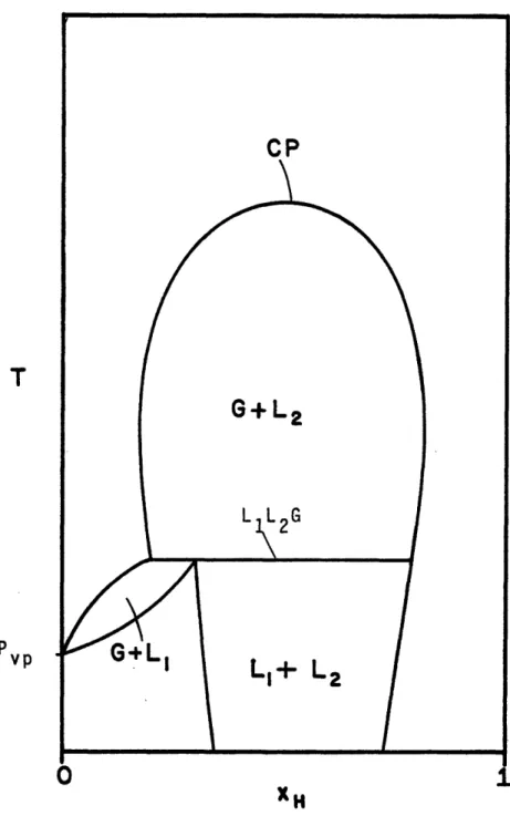
Solubility effects in a supercritical fluid are best illustrated by example. Figure 1.1 gives a solubility "map" for the system naphthalene - carbon dioxide near the critical point of carbon dioxide. Tracing a particular isobar in this diagram shows how the concentration of naphthalene in the carbon dioxide fluid phase varies with temperature. The lines in the diagram represent saturated solutions, i.e., there is always a pure solid naphthalene phase present (naphthalene's normal melting point is 80°C). Above about 75 atm an isobar gives the composition of a saturated CO₂ fluid in equilibrium with solid naphthalene. For any lower pressure, there is a temperature at which three phases coexist - pure solid, saturated liquid, and saturated vapor. The composition of the saturated liquid and vapor at 65 atm are shown in the figure by a tieline; the locus of all these tieline compositions for various pressures is given by the dashed line. If 'the solid-liquid-vapor (SLV or SLG) locus is traced to higher temperatures (and pressures), it is found that the liquid-vapor tielines converge to the critical point labelled in the diagram. At this point the near-critical liquid and near-critical vapor phases become indistinguishable, or, in other words, the vapor-liquid critical phenomenon is observed in the presence of a solid phase. The occurrence of the critical phenomenon between two phases in the presence of a third characterizes a special class of critical points known as critical end points. The critical point in Figure 1.1 is known as a lower critical end

(21)

Liquid

Critical Point(LEP·

/ J / / / / 90 80 70 atm.

tie line

Figure 1.1. The experimental solubility map for the

naphthalene (N) - carbon dioxide system. Isobars indicate the mole fraction of naphthalene in solution. The dashed line corresponds to a three-phase solid-liquid-vapor equilibrium. This equilibrium terminates at LCEP, the lower critical end point.

10

10- 3

)

I

(22)

point (LCEP), a designation which will become clear in the following sections.

The effects of temperature and pressure on solubility may be observed in Figure 1.1. Along the 300 atm isobar, solubility increases continuously with temperature due to the increasing activity of the solid phase. At 55 C, the concentration of naphthalene in the supercritical fluid phase is about 5 mole percent, or 15 weight percent. While this compares unfavorably with traditional nonpolar solvents, it is nevertheless a significant quantity of naphthalene.

At 80 atm, solubility decreases sharply with temperature at about 35 C. This is the near critical region, where a slight increase in temperature leads to a large decrease in the density of the fluid. The fluid phase naphthalene concentration drops as the CO₂ loses much of its solvent power. Moving beyond the critical region toward higher temperatures, the density changes again become small and the isobar reverts to a positive slope.

1.3. Phase Diagram

A full understanding of phase behavior in the supercritical fluid region requires an understanding of its

(23)

figure contains the P-T diagrams of the two pure components A and B which comprise the system, and these are of the usual shape. The sublimation, fusion, and vaporization curves for each component meet at the triple point. The vaporization curves terminate at pure component critical points. The other lines in the diagrams represent univariant states of mixtures of A and B. The dashed line connecting CPA and CPB represents the mixture critical line. Composition varies along this line from pure A to pure B. There are four three-phase lines shown, SASG S SBL (eutectic line), SALG, and S LG. These lines all intersect at the quadruple point

B

Q, where the four phases S , G, L, and S all coexist at the

A B

same temperature and pressure.

For systems where the solubility of solid B in the liquid phase is very low, and the temperature of TPB is higher than that of CP , the S LG liquid phase near the

A B

quadruple point is almost pure A. When this low solubility persists to temperatures above the critical point of A, the SLG line cuts the LG critical locus to give a lower critical end point (LCEP) as shown in Figure 1.3. The segment of the SBLG line starting from TPB similarly intersects the

(24)

T

Figure 1.2. The P-T projection for a system in which the liquid phases are completely miscible, and the solid phases are completely immiscible. Triple points are denoted by TP and the quadruple point by Q. S_A and S_B are the pure solids.

(25)

Figure 1.3. The P-T projection of a system in which the gas-liquid critical line is cut by the SBLG line. The length of the lower critical line has been greatly exaggerated. The LCEP is typically within a few C of CPA .

(26)

critical line at an upper critical end point (UCEP). At temperatures between the critical end points, the fluid phase critical phenomenon is not observed at any pressure. Consequently, this region is designated as the supercritical fluid region. The critical point in Figure 1.3 was, as noted, a lower critical end point. An upper critical end point did not appear in that diagram.

1.4. The Euation f State

Generation of phase diagrams of the type shown in the previous section requires fugacity expressions for the solid phase and for a component in a fluid phase. The first of these is easily obtained from an equation for the sublimation pressure of the 'solid. To represent the gaseous, fluid, and liquid phases present, the Peng-Robinson (P-R) equation of state was used. This equation was felt to represent the best compromise between simplicity and accuracy in attaining the desired goal.

The P-R equation is

RT a

(27)

pressure and temperature are specified. Using equation (1.1), an expresssion for the fugacity of a component in a mixture may be derived and used in the calculation of phase equilibria. For a binary system, an empirical interaction parameter, 612 must often be employed to obtain reasonable agreement with experimental data.

1.5. Theoretical Aects

Equilibrium of phases requires that the phases be of equal temperature and pressure, and that the fugacity (or chemical potential) of a given component be the same in every phase. It has been found that plots of fugacity versus composition, at constant temperature and pressure, provide an excellent means of visualizing the criterion of equal fugacities. Consider Figure 1.4, which is a plot of n-hexadecane (subscript H) fugacity versus n-hexadecane mole fraction for the n-hexadecane -carbon dioxide system, at a temperature of 300 K and a pressure of 0.1 atm. The systems represented by this diagram are a result of mixing liquid

(28)

V1 V2

X X X

log xH

Figure 1.4. An f-x plot for n-hexadecane - carbon dioxide. Segment G is the gaseous root, segment U is the mechanically unstable root, and segment L is the liquid root. Segments U and L start at the slope infinity and continue to the pure hexadecane axis.

(29)

unity and an intercept at the pure C16 axis of 0.1 atm. This is the equivalent of ideal gas behavior, since

fH HP =PH (1.2)

where PH is the partial pressure of C16. The second curve appears when the cubic equation (1.4) gives three real

df

roots. In the composition range from the infinity in to dxH xH= 1, segment G corresponds to the high volume (gaseous) root, segment L to the low volume (liquid) root, and segment U to the middle volume root. Between the slope infinity and

df

x ,

-

for segment L is negative, indicating that the

man dxH

liquid phase is materially unstable in this composition

range. For xH greater than xmin, dx_H and segment L represents a stable or metastable liquid phase. Segment U appears to be materially stable in this plot. As with the middle volume root for pure component systems, however, it violates the criterion of mechanical stability (i.e.,

(30)

(p)

> 0) and thus does not represent stable conditions. As indicated by the crossing of segments G and U in the graph, the middle volume root does not always give the middle fugacity root.

Suppose now that suitable quantities of C and CO

16 2

are present in the system so that two phases exist with compositions x and x , and fugacity f H The f-x plot shows that xL must lie between xmin and xH = 1, and furthermore, that fH is between f (xmin) and fH(XH = 1). For the

H H min H H

coexisting vapor phase, which must lie on the straight line segment, equality of fugacities requires that

V < < (1.3)

This limiting procedure illustrates the usefulness of the f-x plots in determining two phase equilibrium, and is one of the steps in the phase equilibrium algorithm developed in this thesis. To find the actual compositions for VLE, it is of course necessary to match partial fugacities of carbon dioxide as well.

Fugacity-composition plots may have many shapes other than that given in Figure 1.4. Figure 1.5 depicts an f-x curve with a closed loop, chosen to illustrate a special case of phase stability discovered in this work. Generally speaking, if one starts with a stable system and moves

(31)

f Un 2

0

x 0 .w~ _l.0010 _.0015 .0020 XH

Figure _{1.5. A Cartesian plot illustrating the closed} loop behavior of the fH- _{xH curve at conditions near CO2's vapor}

pressure.

(32)

continuously toward the limit of stability, the highest order stability criterion will be the first (or among the first) to be violated. For binary systems, this means that a stable system will violate the criterion of material stability before the criterion of mechanical stability, so that it is sufficient to check only the former to ascertain phase stability. This is shown in Figure 1.5 by tracing the stable gaseous root with increasing x. At fmax' the material

dfH

stability criterion is violated as dx becomes negative. dxH

The mechanical stability criterion is not violated until the composition of the slope infinity is reached. A special case arises, however, when the stable gaseous or liquid root is traced with decreasing x_{H .} Since all three roots join at the origin, it is possible to follow segment G or L to xH = 0, and then proceed with increasing xH along segment U. In this instance, the mechanical stability criterion has been violated without a violation of the material stability criterion. In light of this possibility, a discontinuity in

df

dH must be treated as a violation of the stability dxH

criterion. Upon tracing a stable system through such a discontinuity, it is necessary to evaluate all stability criteria, not just the one of highest order, to determine phase stability.

Fugacity-composition plots may be used in the

(33)

Axx xv 2

L1

= A A x A A - A > 0 (1.4)

Ax A XV

XV VV

For a stable system, L>O. At the limit of stability, i.e., on the spinodal curve, Ll=O. Spinodal points correspond to extrema in an f-x plot. The L1 criterion is not strictly

df_H

equivalent to the H criterion since these two quantities dXH

differ in sign in a region of mechanical instability. For this reason, it is best to treat material stability as undefined in a region of mechanical instability. The second criterion of criticality is

A A

VV XV 2

Ml=a1

_Ml

_Ll

_aL

L=A A

_AXXX

_VV

A -

_VVVXXXV

AvvvAxxAxv

3A Avv

_VVXVVXX

xvAvxx

av ax

2

+ 2Ax + A

wAvvxAxx

-

(1.5)

Points of M=0 correspond to inflection points in an f-x plot. At a critical point, both L1 and M equal zero. This

(34)

work has shown that the M=0 criterion may be replaced by the

criterion aL1 = 0 in critical point determinations. T,P

This must be so because a critical point is a terminus of a spinodal surface. As the critical temperature and pressure are approached, two points of L1=0 may be brought arbitrarily close to one another in composition. At the critical point, the two L1 zeroes coincide (see Figure 1.10).

1.6. The n-Hxadecane - Carbon Dioxide System

The considerations of the preceding sections make it possible to determine overall phase behavior in binary systems, provided sufficient data is available to allow the choice of an appropriate interaction parameter. For the C_{1 6} - CO2 system, P-T measurements along the upper critical line provide the requisite information. Figure 1.6 shows the upper critical line generated for various values of 612

(using the L1=0 and M1=0 criteria), and illustrates the marked effect of this parameter on the predictions. The experimental upper critical line starts from the critical point of C_{1 6}, rises to a pressure maximum, falls to a pressure minimum, and thereafter runs steeply to higher pressures and temperatures. On the basis of this curve, a

(35)

30

E

O-20

10

300

400

500

600

700

T, K

Figure 1.6. The P-T projection for the C_{1 6}-C0₂ system showing the effect of 612 on the predicted upper critical line. The pure C 2 critical point has also been included, although it is

(36)

No solids form in this pressure and temperature regime.

Figure 1.6 includes the critical point of C0₂, which serves as a starting point for the lower critical line. Figure 1.7 is an enlargement of the P-T projection in this region. The lower critical line intersects the three-phase L₁L₂G line at an LCEP analogous to that shown in Figures 1.1 and 1.3. Now, however, the liquid-vapor critical phenomenon

occurs in the presence of a second liquid phase. The critical line continues past the LCEP in a metastable fashion, until being terminated at a cusp by the unstable critical line. The unstable critical line is the terminus of an unstable binodal surface.

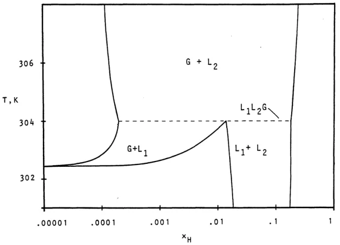
The three-phase line in Figure 1.7 is predicted by noting the intersection of binodal curves at a given temperature or pressure. Figure 1.8 illustrates qualitatively the shape of the T-x section expected on the basis of the measured critical loci. The three binodal regions intersect at a common temperature to give a three-phase L₁-L₂-G tieline. At the high temperature end, the G-L₂ region terminates at a point along the upper critical line. The G-L₁ region, on the other hand, terminates at the CO2 vapor pressure point (i.e., the boiling point of C2 at 70 atm). The L1-L₂ region extends off the plot to lower temperatures, where it will eventually terminate due to solid formation.

(37)

80 P(atm) 75 70 65 300 305 310 315 T(K)

Figure 1.7. The P-T projection of the lower critical line for C16-C02. The stable critical line is metastable between LCEP

(38)

P

XH

(39)

predicted at 304 K. Although the predicted diagram is qualitatively correct, it is incomplete, because the P-R equation generates metastable and unstable phase equilibrium solutions in addition to the stable solutions which are shown.

Figure 1.10 gives the T-x section when all phase equilibrium solutions from the P-R equation are drawn in. The binodal curves are labelled by number pairs which refer to particular monotonic segments of the f-x curve from which the equilibrium arises. Figure 1.11 gives a typical f-x plot for this region' showing the numbering of the monotonic segments. Comparison of Figure 1.10 with Figure 1.9 indicates that the G-L2 region is represented by the (1,7) binodals, the G-L1 region by the (1,5) binodals, and the L -L region by the (5,7) binodals. Note that a significant

1 2

portion of the stable (1,5) binodals falls in a region bounded by two spinodal curves. Stable solutions appear in this nominally unstable region because of the existence of multiple roots to the cubic. Each of the stable binodals

(1,5), (1,7), and (5,7) continue in a metastable fashion past the three-phase line to reach a maximum or minimum

(40)

.00001 .0001 .001 .01 .1 1

XH

Figure 1.9. The predicted T-x section for C16-C02 at 70 atm, in the vicinity of the three-phase line.

306

T,K 304

(41)

.0001 .001 .01 .1

x

H

Figure 1.10.The T-x section at 70 atm showing the continuation of the predicted binodal curves. Each binodal is labelled with a number pair to indicate which segments of the f-x curve the equilibrium is derived from. To determine the compositions of coexisting phases, a tieline is drawn at constant temperature

joining binodals labelled with the same number pair. Note that the three-phase tieline (dashed) joins the two curves labelled (1,7), the two curves labelled (1,5), and the two curves labelled (5,7). The spinodal curve (Ll=0) is given by the heavy lines. At the

/

a(L1=0)

unstable critical point, both

)

and - are zero.

ax T,P ax TP 307 306 305 304 303 302 301 . OD0I

(42)

0.00001 0.0001 0.001 0.01 0.1 1

XH

Figure 1.11. An f-x plot in the three-phase region, showing the

numbering of the seven monotonic segments.

-3 -4 -5 0 -6 -7 -8 -9

(43)

0.00001 0.0001 0.001 0.01 0.1

Figure 1.12. The P-x section at 463.1

E

4-QO_v

K.

(44)

temperature. At a temperature extremum, the metastable binodal joins an unstable binodal locus. There are three

separate continuous curves in Figure 1.9. The first two follow the course (1,7)-(3,7)-(4,7)-(5,7), and the third the course (1,5)-(1,6)-(3,6)-(4,6)-(4,6)-(3,6)-(1,6)-(1,5). This last curve exhibits an unstable critical point where the two (4,6) branches join. Reference to Figure 1.11 shows that both segments 4 and 6 are materially unstable.

A small amount of low pressure P-T-x data is available for the C1 6 - C02 system. Figure 1.12 gives a typical comparison between this data and predictions with 612 = 0.081. On the basis of the lean component, errors in the C02-rich phase are less than fifteen percent, while those in the C -rich phase are less than twenty-five percent. On

16

the basis of the rich component, the errors are less than 1 and 5 percent, respectively. This agreement is quite good considering that no composition data was used in the determination of the interaction parameter.

1.7. The Naphthalene - Carbon Dioxide System

The naphthalene (N) - carbon dioxide system adds the complication of pure solid formation to the phase diagrams.

(45)

parameter. The predicted curves all have the correct general shape and for the most part are within a factor of two of the experimental values. It is evident that a pressure dependent

interaction parameter is needed for quantitative agreement. Figure 1.14 shows the comparison of predictions and experiment at 550C. The three lowest values of the interaction parameter predict a sudden jump in the solubility of naphthalene and thus show a large discrepancy with the measurements. The solubility jump occurs because the P-R equation predicts a phase transition. Figure 1.15 gives a more complete picture of the P-R predictions at 55 C for a value of 612 - 0.11. The solubility jump is seen to correspond to the S-L-F tieline, as the equilibrium system shifts from solid-fluid to solid-liquid. Note that the data are well correlated by the metastable S-F line to pressures over 300 atm.

The solubility jump of Figure 1.14 is experimentally observed at temperatures above 550C. Figure 1.16 compares predictions and measurements at 64.90C. Data taken after the solubility jump exhibited a great deal of scatter due to the presence of more than one phase in the CO2 stream being

(46)

250 ]o

P (atm)

solubility of naphthalene in supercritical

P (atm)

Figure 1.14. CO₂ at 550C. is predicted

The solubility of naphthalene in supercritical For 12' 0.09, 0.10, and 0.11, a solubility jump by the P-R equation. log xN 10n seo Figure CO2 at 1.13. The 450c. log xH

(47)

O A U) C --o/ 0. C D Cb m OUN O 0 Q-U) - ) - _ L N I I I I

0

o Hl U-' U' 1I. I rl 54 CY0 .4 N r-n II 54

(48)

0 r Nr r ! I I I I t~3 0 Hl El 0 0 cq CD c -o c e4-0 -o -0 el

7

_a)

(49)

L-With the same interaction parameter, the P-R equation generates the solubility map shown in Figure 1.17 This is to be compared with Figure 1.1. The qualitative picture of phase behavior in the S-L-G and supercritical fluid regions is excellent. The P-R prediction of an S-L-F three-phase region terminated by an upper critical end point (cf. Figure 1.3) has been included. The UCEP pressure and mole fraction of naphthalene are both much higher than for the LCEP.

Figure 1.18 shows the naphthalene - CO₂ P-T projection, which is to be compared with Figure 1.3. For

naphthalene - CO 2, the critical line is tending toward higher

pressures at the UCEP. This indicates that, even had the solid phase not precipitated out, liquid-liquid immiscibility would preclude the occurrence of a continuous critical line between the two pure component critical points. The inset shows the course of the lower critical line (dashed) which terminates at the LCEP. This is the LCEP which appears in Figures 1.1 and 1.17. Unfortunately, there is no data available over most of the pressure and temperature range covered by Figure 1.18. To allow some judgment of its

(50)

T (K)

280 290 300 310 320 330 340 350 360

Figure 1.17. The predicted solubility map for naphthalene - CO

2 .

0 -1 -2 log XN -3 -4 -5

(51)

700 600 500 400 300 200 100 n 300 400 500 600 700 T(°K)

Figure 1.18. The P-T projection for the naphthalene - carbon dioxide system. The range of temperatures between the LCEP and the UCEP is the supercritical fluid region.

(52)

accuracy, the naphthalene-ethylene system was studied.

1.8. The Nahthalene - Ethvlene System

Considerably more experimental data is available for naphthalene - ethylene than for naphthalene - CO2, allowing a better evaluation of the correctness of the predicted P-T-x space. In order to draw an analogy between the predictions for naphthalene - ethylene and those for naphthalene - CO2, the interaction parameter for this system was selected on the basis of data in the supercritical fluid region. A value of

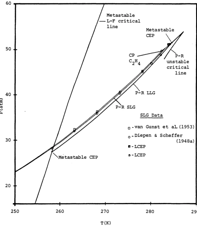
612 = 0 is found to give predictions and agreement similar to Figures 1.13 and 1.14. Figure 1.19, generated with 612 = 0, shows that qualitative agreement is quite good over the entire range of temperatures and pressures. Unlike the naphthalene - CO₂ system, at the UCEP the upper critical line is tending toward lower pressures. As shown by the metastable continuation of this line, however, there again would be liquid-liquid immiscibility if the solid were not present. The qualitative accuracy of Figure 1.19 is an indication of the qualitative accuracy of Figure 1.18. Figure 1.20, the P-x projection for naphthalene-ethylene, shows the semiquantitative agreement of predicted and experimental phase compositions for the S-L-F three-phase line and the L-F critical line.

(53)

, JI 200 -. 100 300 400 500 600 700 T,K

Figure 1.19. The P-T projection of the naphthalene - ethylene system. The inset shows the region near ethylene's critical point (see also Figure 1.21). Experimental curves are from van Welie and Diepen (1961).

(54)

0 .1 .2 .3 .4 .5 .6 .7 .8 .9 1.0

XN

Figure 1.20. The P-x projection of the upper critical line and the SLF region for naphthalene - ethylene.

300 200 P (atm) 100 CPN TPN

(55)

starts at the solvent critical point and is terminated when it meets the unstable critical line at a cusp. The diagram also depicts the metastable LLG line and metastable L-F critical line. The metastable LLG line terminates at a metastable CEP at either end.

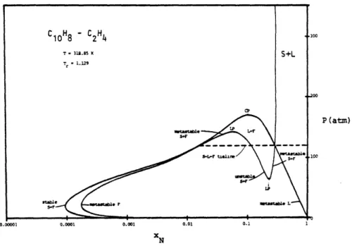
Figure 1.22 illustrates a P-x section for this system at a temperature between the UCEP and naphthalene's triple point. The S-L-F tieline corresponds to a point along the three-phase S-L-F line in Figure 1.19. Note that the solid-liquid and solid-fluid binodals are part of a single curve with metastable and unstable portions. The L-F binodal has a stable critical point, but is metastable below the tieline. At the UCEP the L-F binodal falls entirely within the S-F binodalt except for the critical point, which intersects the S-F binodal at a point of horizontal inflection. This is shown in Figure 1.23. The horizontal inflection point in the stable binodal is a necessary and sufficient criterion for the occurrence of a critical end point. This is true not only for SLF or SLG critical end points, but also for LLG critical end points in the C - CO

16 2

(56)

Mu 50 40 Pi 30 20 250 260 270 280 290 T(K)

Figure 1.21. The P-T projection of the naphthalene - ethylene system in the vicinity of ethylene's critical point.

(57)

Figure 1.22. A P-x section between the UCEP and naphthalene's triple point.

XN

Figure 1.23. The P-x section temperature (approximately). of horizontal inflection.

at the upper critical end point The S+F binodal exhibits a point

(58)

The presence of the LLG line in Figure 1.21 and the liquid-fluid binodals in Figure 1.22 emphasize the fact that the P-R equation predicts a complete fluid phase diagram for the system, and does not indicate the formation of solid. Solid phase equilibrium lines only result when the expression for solid fugacity is introduced, and these lines are in essence superimposed on the fluid phase diagram.

1.9. The Benzene - ater System

An interaction parameter for the benzene - water system was determined by matching the P-T coordinates of a single point along the experimental upper critical line. Figure 1.24 shows the critical line predicted for two different values of _{1 2}; the value chosen was 612 = 0.052. Although the upper critical line apparently exhibits the correct behavior, some qualitative discrepancies are encountered in the region of the lower critical line. Figure 1.25 shows the experimental P-T projection in the vicinity of benzene's critical point. The lower critical line begins at the benzene critical point, reaches a minimum temperature, and shortly thereafter intersects the LLG line at a critical end point. The dashed line represents the metastable continuation of the critical line. This "hypothetical"

(59)

H20 2-.052 O Alwani 570 580 590 600 610

T(K)

620 630 640

Figure 1.24. The P-T projection of the upper critical locus for benzene - water. The predicted curves are actually two separate segments (see Figures 125 and 1,27),

600, 500 P(atm) 400. 300. 200. 100-n C6H6 0critical point 560 VZ _ _ . . _ . I _

(60)

a)

0 r f

o a Um 0 0 - *H 4 -4 cJ r 0 0 O ) *, 0 ,-- *H U I ) H P4 N H a) o a o , *r _{4 4} O~ a) a) a 0 * *H = H CN 04) P II I

(61)

regions, rather than three binodal regions as in Figure 1.8. As such, three phases would not coexist along this line. However, the line is continuous with the stable LLG line, and represents the course of that line had the critical phenomenon not intervened. The metastable LLG line

terminates at a critical solution end point, simultaneously intersecting the L-L and L-G critical lines. The transition between the L-L and L-G critical lines has been drawn as smooth, although experimental measurements indicate that this is not actually true. No measurements of the L-L critical line are available in this region to indicate its correct shape, however.

Figure 1.27 gives the calculated P-T projection in the vicinity of benzene's critical point. The critical curve starting from the pure water critical point (cf. Figure 1.24) does not intersect the liquid-liquid critical line, but rather reaches a minimum in temperature and then returns to the benzene critical point. The liquid-liquid critical line on the other hand reaches a minimum in pressure shortly before being terminated by an unstable critical line. The figure also shows the three-phase LLG line which terminates

(62)

0 10 20 30 40 50 60 70 80 90 100 wt % H20

Figure 1.26. A P-x section between the LCEP and benzene's critical point.

(63)

.) al -,4 G; o .) Ln N ia ur ID 4Z O u U o 4 0 Pi &

o

0 * 0 n _UE D ₀ X o ea 0 v-LA 4. o . -4 -'O 4.) 0 -S.) 2 . 04

(64)

0 10 20 30 40 50 60

wt ; H20₂

70 80 90 100

Figure 1.28. A P-x section slightly above the temperature minimum in the G-L critical line of Figure 1.27.

130 120 110 100 90 P(atm) 80 70 60 50 40

(65)

The experimental and predicted P-T projections differ in that the former depicts a metastable portion of the LLG line, corresponding to the intersection of two binodal regions. However, data were taken on a fairly coarse grid, and a third binodal region of limited extent may well have gone undetected. The equation of state predictions indicate that very careful measurements are necessary to determine the stability or metastability of the LLG line up to the critical solution end point. At present it is not possible to say which of the two P-T projections is correct.

Figure 1.28 'gives a predicted P-x section for this system, at a temperature slightly above the temperature minimum in the G-L critical line of Figure 1.27. Note the prediction of a stable azeotrope. Although the experiments were not detailed enough to verify this, a stable azeotrope

necessarily exists in this system.

(66)

Knowledge of the overall phase behavior of systems is of importance in process design, since it indicates under what conditions a phase equilibrium process is most favorably carried out. For example, supercritical extraction of naphthalene with ethylene should probably be carried out near the UCEP rather than the LCEP. Although the pressures required are 3.5 times as high (174 atm versus 51 atm), the solubility of naphthalene is 85 times as high (0.17 versus 0.002 mole fraction). As a further example, suppose it was desired to dissolve benzene in water. The shape of the upper critical line for this system shows that conditions of about 300 C and 170 atm are sufficient to yield complete miscibility of these two substances.

In developing a methodology to predict overall P-T-x diagrams, a number of significant results were obtained. These are as follows:

-Fugacity-composition plots provide an excellent means of representing the possible types of stable and metastable phase equilibrium at a given temperature and pressure.

-If the material stability criterion reaches a point of discontinuity in the tracking of a stable system, that point may represent a limit of mechanical stability. This is true even if the material

(67)

give conflicting information in such a region.

-When the cubic equation has multiple roots, P-x and T-x sections may correctly indicate the existence of stable states within a region bounded by spinodal curves.

-In critical point determinations, the criterion Ml=O may be replaced by the alternate criterion

aLl\

0.

T,P

-An unstable critical point may be identified as the terminus of an unstable binodal locus.

Alternatively, ( x )is TP greater than zero for

a stable critical point and less than zero for an unstable critical point.

-A necessary and sufficient criterion for the existence of a critical end point is the occurrence of a horizontal inflection point in the stable binodal locus in a P-x or T-x section.

-Solution of the two-phase equilibrium problem is sufficient for the determination of three-phase equilibrium, since three-phase equilibrium results

(68)

from the intersection of binodal loci.

From the systems investigated, the following conclusions have been drawn:

-The Peng-Robinson equation, with a single, constant interaction parameter, gives a qualitatively correct representation of phase behavior over the entire fluid region for nonpolar binary systems. The system may be nonideal with respect to molecular size of the

components.

-The Peng-Robinson equation, with a single, constant interaction parameter, gives a reasonably correct representation of phase behavior over the entire fluid region for binary systems with one polar component. The qualitative picture may be incorrect in certain minor details.

-Semiquantitative predictions may be obtained in any region of interest by choosing an appropriate interaction parameter. In particular, the supercritical fluid region is amenable to such treatment.

-Analysis of fugacity-composition plots allows the development of phase equilibrium algorithms suitable

for any region of the phase diagram.

-Metastable and unstable solutions to the phase equilibrium equations are always associated with

(69)

The significance of the last two conclusions for computer calculations of phase equilibrium must be strongly emphasized. Algorithms which fail to account for the behavior of the fugacity functionality are liable to experience convergence problems when this functionality takes on a complex shape. Complex shapes are found in three-phase regions, as well as near azeotropic coordinates and pure vapor pressure curves. Similarly, algorithms which fail to account for all phase equilibrium solutions to an equation of state may converge to an incorrect result. Erroneous prediction of both binodal curves and critical lines may occur. Careful development and application of phase equilibrium algorithms is necessary to avoid these difficulties.

Taken as a whole, the above conclusions indicate that a simple, cubic equation of state is well suited to an orienting or preliminary study of binary phase behavior. The minimal computing time required by these equations makes them an excellent choice for such an application. The preliminary study maps out regions where more detailed investigation, in both the theoretical and experimental sense, is warranted.

(70)

From the theoretical standpoint, once these regions have been defined, it may in some cases be desirable to switch to a more accurate equation of state. In other cases the cubic equation will provide sufficient accuracy with only a change in the interaction parameter. From the experimental standpoint, the preliminary study indicates the regions where further data should be taken, and how carefully it need be taken. It also serves as a check on the consistency of experimental results.

(71)

was motivated by the unique solvent properties exhibited by a substance somewhat above its critical temperature and pressure, known as a supercritical fluid. Supercritical fluid technology is a relatively recent development. Effective evaluation and use of the technology is aided by knowledge of a system's overall phase behavior. The generation of phase diagrams requires firstly a familiarity with the diagrams, and secondly, a mathematical model, the equation of state, as a means of prediction. This chapter includes a survey of these topics.

Chapter 2 considers the theoretical basis for phase equilibrium predictions, and Chapter 3 illustrates these as applied to pure component systems. Chapters 4 through 7 present the results of this work, calculated phase diagrams covering the complete range of fluid phase behavior for four binary systems. Chapter 8 sums up the conclusions drawn from these results, and gives recommendations for future work.

(72)

2.1 Supercritical Fluids

The first published observation of the solubility of solids in supercritical fluids was given by Hannay and Hogarth in 1879. Working with a number of different solutes and solvents, they noted the high sensitivity of the solubility to changes in temperature and presssure. Geochemists, concerned with the transport of minerals below the earth's surface by pressurized steam, were probably the first to realize the practical importance of supercritical phase behavior. Niggli discussed this topic as early as 1912, and by the 1930s, considerable experimental work had been undertaken.

Table 2.1 lists some proposed uses of supercritical fluids which are of interest to the chemical processing industries. Messmore (1943) was apparently the first to suggest an engineering application of supercritical solvents, a process for the removal of heavy components from crude oil. Since that time a number of other supercritical fluid processes have been proposed, but only within the past two decades have these proposals been economically practicable. A milestone was reached in June of 1978, with the convening of the first symposium on extraction with supercritical fluids (Wilke, 1978). That year also saw the industrial commercialization of a coffee decaffeination process using supercritical carbon dioxide, a process discovered by Zosel

(73)

Extraction of lanolin from wool grease Supercritical fluid

chromatography Decaffeination of

coffee

Extraction of coal Enhanced oil recovery Supercritical fluid

chromatography Removal of nicotine

from tobacco

Extraction of 'flavor components from hops, spices & cocoa

Extraction of oil seeds

Regeneration of

activated carbon

Purification of dredge

spoils

Reforming of forest produc

Hydroca rbons

Carbon Dioxide

Toluene Carbon Dioxide Various solvents, e.g.

Pentane, Isopropanol Carbon Dioxide Carbon Dioxide Carbon Dioxide Carbon Dioxide Water :ts Water

Zhuse, Yushkevic, & Gekker (1958) Sie, et al. (1966)

Zosel (1970)

Wise (1970) Huang & Tracht (1974) Klesper (1978)

Hubert & Vitzthum (1978)

Hubert & Vitzthum Modell Modell Modell (1978) (1978) (1979) (1980)

(74)

in 1970.

In theory, any solvent with a chemically stable critical point may be used as a supercritical solvent. Table 2.1 includes the examples of water, toluene, and other hydrocarbons. However, the class of supercritical solvents also includes substances which are gaseous at normal conditions, such as carbon dioxide and ethylene. Table 2.2 (Klesper, 1978) lists critical data for some of the substances which have been suggested for use as supercritical solvents. The state of each substance at ambient conditions is indicated by its boiling point.

Supercritical solvents possess physical properties ranging between those of gases and liquids, and it is for this reason that the term fluid is used. Table 2.3 (Gouw and Jentoft, 1972) lists some typical physical properties of gases, liquids, and supercritical fluids. Note that the table only gives ranges for the properties of supercritical fluids; an important characteristic of a supercritical fluid is that its properties are highly variable for small changes in temperature and pressure.

Table 2.3 indicates that supercritical solvents have a substantially higher self-diffusivity than normal liquids. Higher rates of mass transfer are to be expected in a supercritical solvent, and such an effect has indeed been

(75)

NH3 -33.4 H₂0 100.0 Methanol 64.7 Ethanol 78.4 Isopropanol 82.5 Ethane -88.0 n-Propane -44.5 n-Butane - 0.5 n-Pentane 36.3 n-Hexane 69.0 2,3 Dimethylbutane 58.0 Benzene 80.1 Dichlorodifluoromethane -29.8 Di ch 1 orofl uo romethane 8.9 Trichlorofluoromethane 23.7 1,2-Dichlorotetrafluoroethane 3.5 Chlorotrifluoromethane -81.4 Nitrous oxide -89.0 Diethyl ether 34.6

Ethyl methyl ether 7.6

132.3 111.3 240 374.4 226.8 344 240.5 78.9 272 243.4 63.0 276 253.3 47.0 273 32.4 48.3 203 96.8 42.0 220 152.0 37.5 228 196.6 33.3 232 234.2 29.6 234 226.8 31.0 241 288.9 48.3 302 111.7 39.4 558 178.5 51.0 522 196.6 41.7 554 146.1 35.5 582 28.8 39.0 580 36.5 71.4 457 193.6 36.3 267 164.7 43.4 272 a - Klesper (1978)

(76)

(jl Q) a-r U 0 L CU Ci -I L U LI Q 0 cn cO L I I _· _- I O O O O I I O O O

0

,-._ O _ C -3

₀

o

_o

X 0 Ln l u, -E U, U, E

;L

E 0o ~ ~ I-0 0. i E 4-., - .- U Q t 4- , .-O C _ C > a _{e o}m a _, 9 _{0 0} r0' LL U I.-U 0. :3 , .I -Q) L r ) . CU rC 4-0 t, 4 0y

(77)

I-affinity for a given solute, which determines the solubility of the solute. This affinity, a result of intermolecular attractive forces, is highly dependent upon the distance between molecules. Near the critical point, small changes in temperature or pressure lead to sizeable changes in the fluid density, with concomitant changes in solubility characteristics. This phenomenon is best illustrated by an example.

Figure 2.1 (Modell, 1979) is a solubility "map" for the system naphthalene (C0Hs) - carbon dioxide (CO₂) near the critical point of CO_2. Tracing a particular isobar in this diagram shows how the concentration of naphthalene in the carbon dioxide fluid phase varies with temperature. The lines in the diagram represent saturated solutions, i.e., there is always a pure solid naphthalene phase present

(naphthalene's normal melting point is 800C). Above about 75 atm an isobar gives the composition of a saturated CO₂ fluid in equilibrium with solid naphthalene. For any lower pressure, there is a temperature at which three phases coexist - pure solid, saturated liquid, and saturated vapor. The composition of the liquid and vapor at 65 atm are shown

(78)

0 10 20 T(°C)

30 40 50

Figure 2.1. The solubility map for the naphthalene (N) -carbon dioxide system. Isobars indicate the mole fraction of naphthalene in solution. The dashed line corresponds to a three-phase solid-liquid-vapor equilibrium. This equilibrium

terminates at LCP, the lower critical end point. 10- 1 10-2 XN -3 10 -I I I I I I tm. / tie line I _ ) ]o

(79)

in the diagram. At this point the near-critical liquid and near-critical vapor phases become indistinguishable, or, in other words, the vapor-liquid critical phenomenon is observed in the presence of a solid phase. The occurrence of the critical phenomenon between two phases in the presence of a third characterizes a special class of critical points known as critical end points. The critical point in Figure 2.1 is known as a lower critical end point (LCEP), a designation which will become clear in the discussion of phase diagrams

(Section 2.2).

The effects of temperature and pressure on solubility may be observed in Figure 2.1. Along the 300 atm isobar, solubility increases continuously with temperature due to the increasing activity of the solid phase. At 55 C, the concentration of naphthalene in the supercritical fluid phase is about 5 mole percent, or 15 weight percent. While this compares unfavorably with traditional nonpolar solvents, it is nevertheless a significant quantity of naphthalene.

At 80 atm, solubility decreases sharply with temperature at about 35°C. This is the near critical region, where a

(80)

slight increase in temperature leads to a large decrease in the density of the fluid. The fluid phase naphthalene concentration drops as the C02 loses much of its solvent power. Moving beyond the critical region toward higher temperatures, the density changes again become small and the isobar reverts to a positive slope.

The solubility phenomena in the supercritical fluid region provide the basis for the processes in Table 2.1. With the aid of Figure 2.1, it is easy to imagine how a supercritical fluid extraction process might work. At a supercritical temperature of 450C, for example, CO2 is compressed to 150 atm where it dissolves 2 mole percent of naphthalene from an inert substrate. The SCF carries the naphthalene to a collection vessel, at which point the pressure is reduced to 70 atm or less. The naphthalene solubility is lowered by a factor of 50, and it precipitates out as a pure solid. The CO2 may now be pressurized and recycled. The fact that no distillation or purification step is required for solute recovery often results in an energy savings over conventional extraction operations.

It is important to note the modest pressures and temperatures at which a supercritical CO2 extraction can be carried out. In the example of Figure 2.1, pressures below 300 atm and temperatures in the range of 300C to 600C would be suitable. The low temperature of this process is a main

(81)

This fact is evidenced in Table 2.1. Availability of CO is

2

also a prime consideration in the enhanced oil recovery process of Table 2.1. The American petroleum companies researching this application intend to utilize CO2 from natural underground reservoirs (Stalkup, 1978). The C02 will be pumped from the reservoir to an oil field, where it is injected into the oil bearing substrate. There it solubilizes and displaces the oil to bring it to the surface.

Water is another supercritical solvent with great promise. Its role in geochemical phenomena has been mentioned. Two applications, which appear in Table 2.1, have recently been suggested by Modell. Table 2.4 also gives a number of literature sources pertaining to the solvent properties of supercritical water. The solubility of a hydrocarbon in water will be investigated in Chapter 7, which deals with the benzene-water system.

The preceding paragraphs have indicated the importance and potential of supercritical fluids for chemical engineering applications. Evaluation of new and existing

(82)

Table 2.4

Literature Sources for Supercritical Water

Application Solubility of wood

Solubility of glass (silica) Solubility of hydrocarbons Solubility of argon Solubility of nitrogen Solubility of salts Geochemical aspects Reference Woerner (1976) Martynova (1976) Connolly (1966)

Lentz & Franck (1969)

Tsiklis & Maslennikova (1965) Niggli (1912)