Publisher’s version / Version de l'éditeur:
Journal/American Water Works Association, 98, May 5, pp. 107-115, 2006-05-01
READ THESE TERMS AND CONDITIONS CAREFULLY BEFORE USING THIS WEBSITE.
https://nrc-publications.canada.ca/eng/copyright
Vous avez des questions? Nous pouvons vous aider. Pour communiquer directement avec un auteur, consultez la
première page de la revue dans laquelle son article a été publié afin de trouver ses coordonnées. Si vous n’arrivez pas à les repérer, communiquez avec nous à [email protected].
Questions? Contact the NRC Publications Archive team at
[email protected]. If you wish to email the authors directly, please see the first page of the publication for their contact information.
NRC Publications Archive
Archives des publications du CNRC
This publication could be one of several versions: author’s original, accepted manuscript or the publisher’s version. / La version de cette publication peut être l’une des suivantes : la version prépublication de l’auteur, la version acceptée du manuscrit ou la version de l’éditeur.
Access and use of this website and the material on it are subject to the Terms and Conditions set forth at
Optimizing source water blends for corrosion and residual control in distribution systems
Imran, S. A.; Dietz, J. D.; Mutoti, G.; Xiao, W.; Taylor, J. S.; Desai, V.
https://publications-cnrc.canada.ca/fra/droits
L’accès à ce site Web et l’utilisation de son contenu sont assujettis aux conditions présentées dans le site LISEZ CES CONDITIONS ATTENTIVEMENT AVANT D’UTILISER CE SITE WEB.
NRC Publications Record / Notice d'Archives des publications de CNRC:
https://nrc-publications.canada.ca/eng/view/object/?id=07e3c8c6-f25e-432d-9505-8b8480ce8316 https://publications-cnrc.canada.ca/fra/voir/objet/?id=07e3c8c6-f25e-432d-9505-8b8480ce8316
http://irc.nrc-cnrc.gc.ca
O p t i m i z i n g s o u r c e w a t e r b l e n d s f o r c o r r o s i o n
a n d r e s i d u a l c o n t r o l i n d i s t r i b u t i o n s y s t e m s
N R C C - 4 9 2 6 2
I m r a n , S . A . ; D i e t z , J . D . ; M u t o t i , G . ; X i a o ,
W . ; T a y l o r , J . S . ; D e s a i , V .
A v e r s i o n o f t h i s d o c u m e n t i s p u b l i s h e d i n
/ U n e v e r s i o n d e c e d o c u m e n t s e t r o u v e
d a n s : J o u r n a l / A m e r i c a n W a t e r W o r k s
A s s o c i a t i o n , v . 9 8 , n o . 5 , M a y 2 0 0 6 , p p .
1 0 7 - 1 1 5
OPTIMIZATION OF SOURCE-WATER BLENDS FOR CORROSION AND RESIDUAL CONTROL IN DRINKING WATER DISTRIBUTION SYSTEMS
Syed A. Imran1, John D. Dietz2*, Ginasiyo Mutoti3, Weizhong Xiao4, James S. Taylor5 and V.
Desai6
1
National Research Council of Canada,
1200 Montreal Rd, Bldg. M-20, Ottawa, ON, K1A 0R6, Canada
2,5
Department of Civil and Environmental Engineering, University of Central Florida P.O. Box 162450, Orlando, FL, 32816, USA
3
Timmons Group,
1001 Boulders Pkwy., Suite 300, Richmond, VA 23225, USA
4
Z-Facilitators Inc.,
3251 Progress Dr., Orlando, FL 32826, USA
6
Advanced Material Processing and Analysis Center
University of Central Florida, P.O. Box 162455, Orlando, FL, 32816, USA
* Corresponding Author: Tel (407)8235304, Fax (407)8233315, E-mail: [email protected]
ABSTRACT
Understanding the issues involved when multiple source waters are blended, particularly impact to distribution system water quality is important. A multi-objective technique is demonstrated that will aid in evaluating blends to identify acceptable water quality for simultaneous control of lead, copper, iron and monochloramine levels in distribution systems. Blends of three different
source waters (groundwater, surface water and desalinated water) are evaluated. The modeling results indicate that the different pipe materials often have conflicting water quality requirements for release abatement. Corrosion of copper and lead pipes for instance was increased by increasing alkalinity, whereas increasing alkalinity was beneficial in reducing the release of iron corrosion products from pipes. Increasing sulfates was found to reduce the release of lead, while iron release increased. These conflicting water quality requirements for lead, copper and iron release necessitate the evaluation of the tradeoffs between water quality and the corrosion response.
BACKGROUND
Tampa Bay Water (TBW) is a wholesale supplier of drinking water to six member governments in Florida. TBW was required by the Southwest Florida Water Management District (SWFWMD) to reduce groundwater withdrawals from 158 million gallons per day (MGD) to 121 MGD (1 MGD = 3785.4 m3/d). In order to comply, TBW completed the construction of a 66 MGD surface water
plant and a 25 MGD desalination plant. The present study is part of a tailored collaborative project (TCP) sponsored by American Water Works Association Research Foundation (AwwaRF) and Tampa Bay Water (TBW) to evaluate the effect of blending groundwater, surface water and desalinated water on the deterioration of water quality within the distribution systems. The ongoing TCP uses pipes extracted from actual distribution systems, which are exposed to historical and new water supplies.
The pilot distribution system (PDS) was constructed of aged pipes that were obtained from existing utility distribution systems. The pipes were removed from the member government’s distribution networks, wetted, capped and transported to the pilot site. Once onsite, the pipes were assembled and allowed to equilibrate with groundwater over a period of 5 months. After equilibrium was
established, different blends were introduced into the PDS. The project was divided into 6 phases; each of three months duration (Phase I to Phase VI). Similar blends were used in alternate phases to evaluate the effect of seasonal conditions on the PDS and related water quality impacts.
Pilot source waters. The pilot facility was constructed such that different source waters having
chemical characteristics that simulate different processes could easily be produced. The different pilot processes and their mode of production are shown in Table 1. The finished water qualities from these pilot processes were set to match the existing and future sources of water proposed by TBW. All the source waters were chloraminated and stabilized to maintain a positive Langelier Index.
Pilot distribution system (PDS) design. The pilot distribution system (PDS) was composed of
eighteen different distribution lines. PDS line 1 to PDS line 14 were hybrid lines that have four different materials: PVC, unlined iron, lined iron and galvanized iron pipes. The average length of each hybrid PDS was 91 ft (27.7 m) and was composed of 19 ft (5.8 m) of PVC, 19 ft (5.8 m) of lined iron, 13 ft (4 m) of unlined iron and 40 ft (12.2 m) of galvanized iron pipes in that order. The diameter of the PVC, lined iron and unlined iron pipes was 6 inch (0.15 m) and the diameter of the galvanized iron pipe was 2 inch (0.05 m). PDS line 15 was composed entirely of unlined iron pipe. Similarly PDS lines 16, 17 and 18 were composed of lined iron, PVC and galvanized iron pipes, respectively.
Pilot distribution system operation. The pilot distribution system was operated at a 5 day
hydraulic retention time (HRT) initially (Phase I to III) to simulate dead end conditions. The HRT was changed to 2 days during Phase IV through VI to permit maintenance of chloramine residual. Different source waters and their blends were introduced into the PDS by dosing pumps feeding
individual influent standpipes for each PDS line. The PDS were flushed once a week during the 5 day HRT period and once every two weeks for the 2 day HRT period. The flush velocity was 1 ft/s (0.3 m/s) for at least 3 pipe volumes. Sampling was done once a week at the influent and effluent standpipes for a number of water quality parameters.
Lead and copper corrosion loops. Corrosion loops, which consisted of a 30 ft (9.1 m) copper
tubing of 5/8-inch (0.016 m) diameter, were constructed at the end of the each PDS. A lead coupon was inserted in each of the tubing to simulate the release of lead from solders. To simulate water delivered to the customers, the corrosion units received water after it passed through the associated pipe distribution system. The corrosion loops were flushed with 2 gallons of PDS water every morning. Samples for lead and copper analysis were collected after a 6 hour stagnation time after flushing.
Statistical water quality models. Data obtained from two years of continuous operation was used
to develop statistical nonlinear relationships that described the metal release and residual chloramine in terms of source water quality (single source or blends). This approach aids in making quantitative evaluations based on the blended water quality at any point in the pilot distribution system. It should be noted that the models described here were developed to correspond to the specific operating conditions and geometry of the hybrid pilot distribution systems (PDS). Any extrapolation or predictions for utility use requires a detailed calibration procedure described elsewhere (Taylor et al., 2005).
Copper release model. Based on the PDS data, a nonlinear model was developed for the release
22 . 0 2 1 . 0 2 4 86 . 2 73 . 0 72 . 0 ( ) ( ) ( ) ( ) ) ( − − − = T Alk pH SO SiO Cu (1)
Where, Cu, is the total copper released in mg/L, Alk is alkalinity measured in mg/L as CaCO3,
− 2 4
SO and SiO3 are the sulfates and silica respectively in mg/L, T is temperature in oC. The Lead and Copper Rule (LCR) action level for copper stipulates that 90% of samples have a copper level less than 1.3 mg/L. Therefore the goal would be to find water quality blends that would minimize the release of copper, preferably at some value below the action level. The standard deviation of the copper data was 0.22 mg/L. Based on the standard deviation; a one-tailed Z-statistic for 90% compliance would be 1.28. Assuming a normal distribution, the maximum target average copper release is obtained at 1 mg/L.
Lead release model. A nonlinear model, which incorporates the significant water quality
parameters for lead release was developed from the PDS data as (Taylor et al, 2005)
228 . 0 2 4 462 . 1 726 . 2 677 . 0 ) 25 ( ( ) ( ) ( ) ( ) 027 . 1 − − − − = Alk pH Cl SO Pb T (2)
Where, Pb is total lead released in µ g/L, 2− 4
SO , Cl are the sulfates and chlorides in mg/L and Alk
is alkalinity in mg/L as CaCO3. The model predictions of lead release are specific to the lead
coupon area used in this research. For actual utility use, the model predicted lead release should be multiplied by the ratio of the historical lead release to model predicted lead release for the historical water quality. The action level for lead is 15 µ g/L. A 90% compliance level for lead (standard deviation = 7 µ g/L), would stipulate a goal of 6 µ g/L. Comparison with actual member government lead release data indicated that the model over-predicted the lead release. For purposes of this discussion, this inherent bias in the model towards higher lead values was overcome by
setting the maximum permissible lead release at a value of 10 µ g/L. This modification of the 90th
percentile lead value is believed to better reflect the distribution of lead concentrations that have been experienced in the member governments’ distribution systems.
Apparent color (iron) release model. The unlined iron pipes represent a major source of iron in
the water due to corrosion and release of corrosion products. For the conditions of the study a strong relationship exists between the total iron (Fe) concentration (mg/L) and apparent color (chloroplatinate units or cpu) in the pilot distribution system. This relationship is given as (Imran et al, 2005b; Imran, 2003)
Color Apparent
Fe=0.0132× (3)
Due to the high coefficient of correlation (R2 = 0.82) between apparent color and total iron
concentrations for the conditions of this study, apparent color was used as a substitute measurement for total iron. A color (iron) release model was developed for the hybrid PDS as (Taylor et al, 2005; Imran et al, 2005a; Imran, 2003)
912 . 0 321 . 1 836 . 0 813 . 0 967 . 0 118 . 0 2 4 561 . 0 485 . 0 ) ( 10 ) ( ) ( ) ( ) ( ) ( ) ( Alk HRT T DO SO Na Cl C − =
∆
(4)Where,
∆
C is the increase in apparent color (cpu), Na, 2− 4SO , Cl are the sodium, sulfates and
chlorides respectively in mg/L. Alk is the alkalinity in mg/L as CaCO3, DO is the dissolved oxygen
content in mg/L, T is the temperature in oC and HRT is the hydraulic retention time in days. The
SMCL for iron is 0.3 mg/L and 15 cpu for apparent color. Based on the relationship between total iron and apparent color (Equation 3) the SMCL of 0.3 mg/L would correspond to an apparent color of 22 cpu. However, since the SMCL for color is less than the corresponding level for iron control,
a value of 15 cpu will be sufficient for satisfying both the iron and apparent color SMCL. The model given by Equation 4, predicts the change in color rather than effluent color. Therefore, assuming an influent color of 5 cpu, the maximum permissible color release within the distribution system was set at 10 cpu.
Monochloramine dissipation model. A nonlinear kinetic model for the decay of monochloramine in the PDS was developed based on the PDS data as (Taylor et al, 2005; Arevalo, 2003) ) * * ) 254 * ( exp( ( 20) 2 2Cl NH Cl K UV K A t NH i B W T− + − = (5)
Where KB is the bulk decay constant (cm/hr), KW is the wall decay constant (hr-1), NH2Cl is the
monochloramine concentration at time t (hr) in mg/L as Cl2, NH2Cli is the initial monochloramine
concentration in mg/L as Cl2, T is the temperature in oC and A is the temperature correction
coefficient. Based on the PDS data the bulk decay constant KB was 0.1796 cm/hr, the wall decay
constant KW was 0.0121 hr-1 and A was 1.11 for unlined cast iron pipes. Data from the PDS
indicated that the heterotrophic plate count (HPC) population exhibits an exponential growth when the PDS effluent residual is less than 0.3 mg/L as Cl2 (Taylor et al, 2005). A conservative
chloramine residual of 0.5 mg/L as Cl2 is therefore used as the minimum residual level in this
study. It should be noted that the color release and monochloramine dissipation model were developed for a particular pipe material, geometry and flow conditions that simulate low-flow regions of the distribution system. Any application to the full-scale distribution system requires the model to be calibrated for different flow conditions and pipe geometries. Adjustment of the prediction model for alternative flow conditions and pipe geometries are described elsewhere
(Taylor et al, 2005).
CONFLICTING ASPECTS OF WATER QUALITY GOALS
Traditional optimization involves optimizing water quality, sources and costs of water treatment and supply (Elzenga et al, 1987; Liand and Nnaji, 1983). However, there is no comparable study that evaluates the simultaneous impact of blending water sources on different material in the distribution system. Water quality considerations for the minimization of water quality deterioration within the distribution system raise a number of interesting observations. Corrosion of copper and lead pipes for instance is increased by increasing alkalinity, whereas increasing alkalinity was beneficial in reducing the release of iron products from pipes. Increasing sulfates was found to reduce the release of lead, while iron release was increased. These conflicting water quality requirements for lead, copper and iron release necessitate the evaluation of the tradeoffs between water quality and the corrosion response.
The present study recognizes the need to operate within a range of feasible blends of the three source waters, rather than at a single optimum blend. Depending on the demand and operation of the surface water and desalination plants, different points of connection in the distribution system will receive a different blend of the three sources. Therefore the need is to find a feasible range of blends that would not cause problems of copper, iron or lead release.
CALCULATION OF BLEND WATER QUALITY
The water quality of a blend (WQpB) can be calculated using the mass balance on conservative species (alkalinity, sulfates and chlorides). This can be mathematically expressed as:
∑
= = n i i p i B p xWQ WQ 1 (6) 0 . 1 1 =∑
= n i i x (0≤ xi ≤1.0) (7)where, p denotes the water quality parameter (alkalinity, sulfate, etc.); i denotes the source water (groundwater, surfacewater or desalinated water) and xi is the fraction of the sourcewater i.
For non-conservative species (pH) a different solution technique is required due to interaction with the carbonate system (Trussell, 1971). The pH of blend is usually obtained from a mass balance on the [H+] ions using the relationship H+ −pH
= 10 ]
[ . However, due to the sensitivity of the models for copper (Equation 1) and lead (Equation 2) a more rigorous approach to evaluating the pH of blends was used (Trussell, 1971). This iterative method, demonstrated by Trussell (1971), evaluates the pH of blend of different source waters as function of initial pH, alkalinity, temperature and ionic strength.
Three source waters were selected for the purpose of evaluating the blends. These are conventional groundwater source (GW), surface water (SW) and desalinated water (RO). The water quality of these sources is given in Table 2.
RESULTS AND DISCUSSIONS
The corrosion product release for a particular water quality is estimated using the empirical models developed for copper (Equation 1), lead (Equation 2) and apparent color (Equation 4). The monochloramine decay model (Equation 5) is used to characterize the level of residual needed for microbiological control. Based on action levels for copper and lead, the maximum copper and lead
release were set at 1.0 mg/L and 10 µ g/L respectively. The maximum apparent color release was established at 10 cpu in accordance with the SMCL for both color and total iron release. The minimum monochloramine residual was set at 0.5 mg/L as Cl2 to control heterotrophic plate counts
(HPC).
The variable parameter set in this problem was the fraction of different source waters. The solutions represent different blend ratios for the three different source waters which would consider the conflicting water quality requirements for corrosion control of copper, lead and iron simultaneously. A number of different scenarios were evaluated to determine the feasible blends for each case.
Base Scenario. The TBW surface water plant and desalination plant capacities are 66 and 25 MGD respectively. Assuming that these plants are fully operational and functioning at 100% capacity, the maximum share of demand for the surface water and desalinated water is approximately 41% and 16% respectively of the predicted 158 MGD total demand. However, a study conducted for TBW by the Black and Veatch Corporation modeled the TBW transmission system under a range of conditions (Black and Veatch, 2000). Water quality was predicted throughout the TBW service area. The results of these simulations indicate that some connections could receive desalinated water in the range of 0 – 81%. Similar variations in the range of surface water (0 – 90%) were demonstrated. A distribution system may experience different blends of source waters based on where it is located on the transmission systems. Therefore it was decided that a constraint on source water percentages was not appropriate as long as there is no centralized point of blending.
increments of 2% was evaluated (for example, 0%, 2%, … 100%). For the three source waters a total number of 1325 blend increments were evaluated per scenario. However, for brevity only a few blend combinations are presented here.
Examination of the feasible blends of the three source waters indicates that the maximum contribution of GW should be 60% for control of copper release (Table 3). The upper limit on GW contribution is attributed to the increased copper release at higher alkalinities associated with the GW source. The maximum contribution of RO at any point should not exceed 56% for control of color release. Whenever the contribution of groundwater is below 40%, the corresponding contribution from RO should be preferably less than 10% to minimize color release. In the absence of GW (GW percentage is 0%), all the blends of SW and RO are corrosive and would have a color release in excess of the goal (10 cpu). The results indicate that the different blends would not have a lead release problem for the water qualities analyzed for this scenario. The highest lead release would be 8 µ g/L at a 40% GW and 60% RO blend. Higher contributions of surface water give lower lead release. This is due to the higher sulfate content of the surface waters in combination with the low alkalinity and chloride content.
For the groundwater and copper piping system employed in this study, blends that contained in excess of 60% groundwater resulted in exceeding the copper action level. It is important to note that the water sources employed in the pilot study were not treated with inhibitors to alleviate copper corrosion. Pilot waters however were stabilized with respect to calcium carbonate solubility.
In the full-scale systems, several of the utilities that were reliant on 100% groundwater prior to the development of surface water and desalination sources also experienced difficulties with the
copper action levels. These full-scale observations are consistent with the present models
developed from pilot-scale testing. The use of inhibitors was practiced by these utilities to reduce copper concentrations.
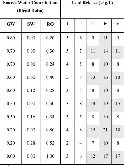
Scenario 2: Effect of Increasing Chlorides. This scenario addresses the variant water quality that could be expected from the desalination plant. A change in chloride and sodium levels could be expected depending on the RO desalination plant product quality. A higher chloride and sodium level may be expected due to membrane deterioration. Therefore, a sensitivity analysis on the chloride levels in the RO product water is necessary. Table 4 and Table 5 show the sensitivity of the color and lead constraints to the increase in chloride concentrations in the RO source. Different levels of chlorides (30, 50, 80 and 100 mg/L) in the RO source were assumed. The results indicate that increasing chloride levels in the RO source could lead to lead release in excess of 10 µ g/L. However, at lower blend alkalinities color is the controlling constraint. Increasing concentrations of chlorides in the RO source require increased alkalinity levels to mitigate the release of color (Imran et al., 2005b). This can be achieved by increasing the percentage of groundwater source in the blend. However, if the chloride concentration exceeds 100 mg/L, the feasibility of using an RO source is reduced.
The commonly used amelioration measure of increasing source water alkalinity (by NaHCO3 salt
addition) was analyzed by increasing the alkalinity of RO from 50 to 80 mg/L. The results indicate that there is are not significant changes in the feasible blend range for color and lead compared to the base scenario. Alkalinity amendment can be counter-productive as it could lead to increased release of copper.
apparent color release, therefore all of the remaining supply should be met with the surface water source. Since even a 100% SW would give a color release greater than 10 cpu, the only remedial approach would be to decrease the HRT. Conversely, none of the blends with RO and SW have a copper violation.
If SW is offline then apparent color is the controlling constraint. The feasible blend indicates that at least 50% of the blend should be groundwater to avoid color problems due to increased RO contribution. GW above 60% would increase copper release beyond 1 mg/L. Therefore, the feasible range would be a narrow range of GW between 56 and 60%.
When RO source is offline, the feasible blend would require at least 20% GW contribution to control color. Simultaneously the GW should be less than 60% to control copper release. This would give a range of groundwater contributions between 20 and 60% that are feasible when RO is offline.
Scenario 4: Effect of pH and HRT. The analyses indicate the complexity of controlling blends of different sources to satisfy often-conflicting constraints. There is a very narrow range of blends that will concurrently satisfy all the goals. This is due to the source water characteristics as well as due to the impact of pipe material. Groundwater is high in alkalinity which is beneficial for controlling iron release but is detrimental to copper and lead release. Controlling the pH of groundwater, or the blend could help in controlling copper and lead release. Table 7 shows the effect of increasing the pH of groundwater on the feasible range for copper control. Increasing the groundwater pH from 7.6 to 7.9 increases the acceptable contribution of GW from 30 to 60%. However, it should be noted that the high alkalinity and calcium content of the groundwater may aggravate scaling and deposition in the distribution system if pH is elevated.
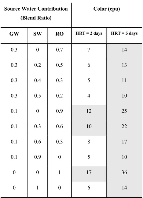
Decreasing the HRT from 5 to 2 days does not affect the maximum GW percentage as it is controlled by copper release and is fixed at 60%. However, maximum RO percentage that can be used is 86%, compared with 56% at a 5 day HRT.
Decreased HRT is also beneficial to maintain a chloramine residual above the targeted 0.5 mg/L as Cl2. The average chloramines residual at a HRT of 5 days was around 0.1 mg/L as Cl2 for all the
blends. When the HRT is decreased to 2 days the average chloramines residual increased to 0.9 mg/L as Cl2. It can be observed from Equation (5) that UV-254 and temperature are the only water
quality parameters that were found to significantly effect chloramine dissipation. However, since both UV-254 and temperature cannot be easily controlled without significant changes to treatment processes or distribution system, controlling residual requires controlling the hydraulic residence time (HRT) in the distribution system. Therefore, a control of monochloramine in the distribution system should be accomplished by a regulation of HRT.
A combination of measures (pH elevation and HRT reduction) could increase the acceptable range of blends. However, unless a separate blending tank is provided, it would be difficult to control the water quality of the blended water for satisfying all the objectives. Where considerable variation in water quality is expected, the use of corrosion inhibitors would be advantageous, especially for mitigation of copper and lead release. It has been demonstrated that copper violations may be expected at GW contributions in excess of 60%. Since the maximum anticipated production capacity of TBW surface water and desalination is limited at 41% and 16% respectively, it would be difficult to control GW contribution below 60% to all the member government. Therefore, due to production limitation on TBW surface water and desalinated water it is necessary to have some measure for mitigation of copper release.
Cost analysis was not covered in this research as the authors intended to focus on the water quality criteria alone. The statistical models identified in this research are based on the assumption of fixed pipe geometry and low-flow conditions. Therefore interpolation to larger distribution systems would require calibration of the models.
CONCLUSIONS
Data from a pilot distribution system was used to develop models for copper (Equation 1), lead (Equation 2) and iron release (Equation 4). These models were used to analyze different blends of three source waters (groundwater, surface water and desalinated water) to identify a feasible range of blends that satisfy the water quality required for control of copper ( ≤ 1.0 mg/L), lead ( ≤ 10
µ g/L) and color ( ≤ 10 cpu) release.
GW contributions greater than 60% lead to unacceptable copper release, due to effect of alkalinity and pH. GW contributions less than 20% lead to unacceptable release in color due to decreased alkalinity.
Higher percentages of groundwater are compatible with higher percentages of the desalinated water (RO) source. The adverse effect of increased chlorides in the RO water on color release is mitigated by a higher alkalinity in the GW source. However, blends of only GW and RO were limited to a maximum RO contribution of 44% to control color release.
Blends with high contributions of RO and SW should be avoided. The high sulfates in the SW and high chlorides in the RO can form a very corrosive blend.
Change in HRT can change the blend requirements significantly. A decrease in HRT from 5 to 2 days increases the chloramines residuals, while decreasing the color release.
The limitations on source water production capacities for the TBW surface water and desalinated water may require the use of corrosion inhibitors to control copper release in those situations where the groundwater contribution exceeds 60% of the blend.
The optimization model was developed for fixed pipe geometry and low flow conditions. However, application to higher flow rates (such as experienced in actual distribution systems) would require full-scale calibration of the model.
ACKNOWLEDGEMENTS
The authors specially acknowledge Christine Owen, Tampa Bay Water Authority Quality Assurance Officer, who was the TBW Project Coordinator, and Roy Martinez, AWWA Research Foundation Senior Account Officer, who was the AwwaRF Project Officer, and the following Member Governments: Pinellas County, Hillsborough County, Pasco County, Tampa, St. Petersburg, and New Port Richey. Pick Talley, Robert Powell, Dennis Marshall and Oz Wisener from Pinellas County, and Dr. Luke Mulford from Hillsborough County are also specifically recognized for their contributions. Several UCF Environmental Engineering students and faculty also contributed significantly to this project and are recognized for their efforts.
REFERNCES
1. Arevalo, J.M. (2003). Modeling the effect of pipe material, water quality and time on
chlorine dissipation. MS. Thesis, Univ. of Central Florida, Orlando, Fla.
2. Black and Veatch Corporation. (2000). Water quality blending analyses: Tampa Bay
Water. Black and Veatch Corporation, Kansas, MD.
of different qualities. Water Supply, 5(3/4), 9-12.
4. Imran, S.A. (2003). The effect of water quality on red water release in drinking water
distribution systems. Ph.D. Dissertation, Univ. of Central Florida, Orlando, Fla.
5. Imran, S.A., Dietz, J.D., Mutoti, G., Taylor, J.S., and Randall, A.A. (2005a). Modified Larsons ratio incorporating temperature, water age, and electroneutrality effects on red water release. ASCE Journal of Environmental Engineering, xx(xx), xx-xx, article in press. 6. Imran, S.A., Dietz, J.D., Mutoti, G., Taylor, J.S., Randall, A.A., and Cooper, C.D. (2005b).
Red water release in drinking water distribution systems. Jour. AWWA, 97(9), 93-100. 7. Liang, T. and Nnaji, S. (1983). Managing water quality by mixing water from different
sources. Jour. Wat. Res. Planning and Mgmt, 109(1), 48-57.
8. Taylor, J.S., J.D. Dietz, A.A. Randall, S.K. Hong, C.D. Norris, L.A. Mulford, J.M. Arevalo, S. Imran, M. LePuil, I. Mutoti, J. Tang, W. Xiao, C. Cullen, R. Heaviside, A. Mehta, M. Patel, F. Vasquez and D. Webb. 2005. Effects of blending on distribution system
water quality. 91065F, AwwaRF, Denver, CO.
9. Trussell, R.R. and Thomas, J.F. (1971) A discussion of the chemical character of water mixtures. Jour. AWWA, 63(1), 49-51.
10. Xiao, W. (2004). Effect of source water blending on copper release in pipe distribution
system: Thermodynamic and empirical models. Ph.D. Dissertation, Univ. of Central
Florida, Orlando, Fla.
AUTHOR TAGLINE
at the National Research Council of Canada. He is currently involved in research on regulatory compliance and water quality impacts on distribution infrastructure integrity at the Urban Infrastructure-Buried Utilities section of Institute for Research in Construction. Syed A. Imran, Ginasiyo Mutoti and Weizhong Xiao earned their Ph.D. from the University of Central Florida. John D. Dietz is associate professor and James S. Taylor is the Alex Alexander Professor and Director of Environmental Systems Engineering Institute at the Department of Civil and Environmental Engineering, University of Central Florida. Vimal Desai is Professor and Director of the Advanced Materials Processing and Analysis Center at the University of Central Florida
Table 1. Mode of production of simulated source waters*
Source waters
Method of Production
GW Aeration of raw groundwater representing historical groundwater usage SW Ozonation and subsequent treatment with BAC of Hillsborough river surface
water coagulated with ferric sulfate, settled and filtered. This simulates the TBW surface water treatment facility
RO Reverse osmosis membrane permeate of raw groundwater, with addition of ocean salt to simulate desalination. This simulates the TBW reverse osmosis desalination plant
*
All waters were stabilized to positive Langelier Index and chloraminated
BAC – biological activated carbon, GW – Groundwater, RO – Desalinated water, SW – Surface water, TBW – Tampa Bay Water
Table 2. Water quality of the source waters used in the simulation. Source Water GW SW RO Alkalinity - mg/L as CaCO3 225 50 50 Calcium - mg/L as CaCO3 200 50 50 Conductivity - µ S/cm 514 589 410 Dissolved Oxygen- mg/L 8 8 8 HRT - days 5 5 5 pH 7.9 8.2 8.3 Silica - mg/L 14 7 1 Sodium - mg/L 10 15 30 Chloride - mg/L 15 10 50 Sulfates - mg/L 10 180 30 Temp - oC 25 25 25 UV254 - cm-1 0.074 0.038 0.024
Table 3.Summary of feasible blends for source water qualities shown in Table 2.
%SW = 100 – (%GW + %ROMax)
%GW %ROMax Controlling
constraint > 60 Copper 50 None 40 34 Color 30 18 Color 20 6 Color < 20 0 Color
Table 4. Effect of chloride content in RO source on color release*
Source Water Contribution (Blend Ratio)
Color Release (cpu)
GW SW RO i ii iii iv v 0.60 0.00 0.40 5 7 10 12 10 0.50 0.20 0.30 6 8 10 12 10 0.40 0.00 0.60 7 11 17 21 16 0.40 0.42 0.18 7 8 10 11 10 0.40 0.48 0.12 6 7 9 10 9 0.30 0.00 0.70 9 14 22 27 20 0.30 0.60 0.10 7 8 10 11 10 0.30 0.62 0.08 7 8 9 10 9 0.00 0.00 1.00 21 36 58 73 41 0.00 1.00 0.00 14 14 14 14 14 *
Shaded regions indicate blends that would release color in excess of 10 cpu. GW – groundwater; RO – desalinated water; SW – surface water
i. RO chloride content = 30 mg/L
ii. RO chloride content = 50 mg/L (base scenario) iii. RO chloride content = 80 mg/L
iv. RO chloride content = 100 mg/L
Table 5. Effect of chloride content in RO source on lead release*
Source Water Contribution (Blend Ratio) Lead Release ( µ g/L) GW SW RO i ii iii iv v 0.80 0.00 0.20 5 6 9 11 9 0.70 0.00 0.30 5 7 11 14 11 0.70 0.06 0.24 4 5 8 10 8 0.60 0.00 0.40 5 8 13 16 13 0.60 0.12 0.28 3 5 8 10 8 0.50 0.00 0.50 5 8 14 19 15 0.50 0.16 0.34 3 5 8 10 8 0.20 0.00 0.80 4 8 15 21 18 0.20 0.28 0.52 2 4 7 10 8 0.00 0.00 1.00 3 6 12 17 17 *
Shaded regions indicate blends that would release Lead in excess of 10 µ g/L. GW – groundwater; RO – desalinated water; SW – surface water
i. RO chloride content = 30 mg/L
ii. RO chloride content = 50 mg/L (base scenario) iii. RO chloride content = 80 mg/L
iv. RO chloride content = 100 mg/L
Table 6. Effect of HRT on color release*
Source Water Contribution (Blend Ratio) Color (cpu) GW SW RO HRT = 2 days HRT = 5 days 0.3 0 0.7 7 14 0.3 0.2 0.5 6 13 0.3 0.4 0.3 5 11 0.3 0.5 0.2 4 10 0.1 0 0.9 12 25 0.1 0.3 0.6 10 22 0.1 0.6 0.3 8 17 0.1 0.9 0 5 10 0 0 1 17 36 0 1 0 6 14 *
Shaded regions indicate blends that would release color in excess of 10 cpu
GW – groundwater, HRT – hydraulic residence time, RO – desalinated water, SW – surface water
Table 7. Effect of groundwater pH on copper release*
Source Water Contribution (Blend Ratio) Copper release (mg/L) GW SW RO i ii iii 1.0 0.0 0.0 1.52 1.26 1.01 0.8 0.0 0.2 1.38 1.13 0.89 0.7 0.3 0.0 1.31 1.07 0.84 0.6 0.0 0.4 1.23 0.98 0.76 0.5 0.0 0.5 1.15 0.91 0.70 0.5 0.5 0.0 1.16 0.93 0.72 0.4 0.0 0.6 1.05 0.83 0.63 0.4 0.6 0.0 1.07 0.85 0.65 0.3 0.0 0.7 0.95 0.74 0.66 *
Shaded regions indicate blends that would release copper in excess of 1 mg/L i. GW pH = 7.6
ii. GW pH = 7.9 iii. GW pH = 8.2