Array processing and forward modeling methods for the analysis of stiffened, fluid-loaded cylindrical shells

Array Processing and Forward Modeling Methods for the

Analysis of Stiffened, Fluid-Loaded Cylindrical Shells

by

Joseph E. Bondaryk

M.S., Electrical Engineering, M.I.T (1988)

B.S., Electrical Engineering and Computer Science, M.I.T (1987) Submitted in partial fulfillment of the

requirements for the degree of

DOCTOR. OF PHILOSOPHY IN OCEANOGRAPHIC ENGINEERING

at the

MASSACHUSETTS INSTITUTE OF TECHNOLOGY

and the

WOODS HOLE OCEANOGRAPHIC INSTITUTION

March 1994

©

All rights reserved.

Signature

of Author

...

...-.

..

...

Joint Program iApplied Ocean Science and Engineering Massachusetts Institute of Technology Woods Hole Oceanographic Institution

Ax~- 8~~8, 1994

Certified by ...

_{""""""""""".~.:..}

_...

Dr. Henrik Schmidt Professor, Massachusetts Institute of Technology

Accpte by.

_

Tesis Supervisor

Accepted

by

... ...

.

...

Dr. Arthur I Baggeroer

Chairman, Joint Committee for Applied Ocean Science and Engineering Massachusetts Institute of Technology/Woods Hole Oceanographic Institution

Array Processing and Forward Modeling Methods for the

Analysis of Stiffened, Fluid-Loaded Cylindrical Shells

by

Joseph E. Bondaryk

Submitted to the Massachusetts Institute of Technology/

Woods Hole Oceanographic Institution

Joint Program in Applied Ocean Science and Engineering on March 28, 1994, in partial fulfillment of the

requirements for the degree of Doctor of Philosopy

Abstract

This thesis investigates array processing and forward modeling methods for the

anal-ysis of experimental, structural acoustic data to understand wave propagation on

fluid-loaded, elastic, cylindrical shells in the mid-frequency range, 2 < ka < 12. The transient, acoustic, in-plane, bistatic scattering response to wideband, plane waves at various angles of incidence was collected by a synthetic array for three shells, a finite, air-filled, empty thin shell, a duplicate shell stiffened with four unequally spaced ring-stiffeners and a duplicate ribbed shell augmented by resiliently-mounted, wave-bearing, internal structural elements.

Array and signal processing techniques, including source deconvolution, array weighting, conventional focusing and the removal of the geometrically scattered contri-bution, are used to transform the collected data to a more easily interpreted

represen-tation. The resulting waveforms show that part of the transient, dynamic, structural

response of the shell surface which is capable of radiating to the far field. Compres-sional membrane waves are directly observable in this representation and evidence of flexural membrane waves is present. Comparisons between the shells show energy compartmentalized by the ring stiffeners and coupled into the wave-bearing internals. Energy calculations show a decay rate of 30dB/msec due to radiation for the Empty shell but only lOdB/msec for the other shells at bow incidence. The Radon Trans-form is used to estimate the reflection coefficient of compressional waves at the shell

endcap as 0.2.

The measurement array does not provide enough resolution to allow use of this technique to determine the reflection, transmission and coupling coefficients at the ring stiffeners. Therefore, a forward modeling technique is used to further analyze the 0° incidence case. This modeling couples a Transmission Line model of the shell with a Simulated Annealing approach to multi-dimensional, parameter estimation. This procedure estimates the compressional wavespeed at 5284m/sec and a compressional decay rate of 49dB/msec. Small cross-coupling coefficients between flexural and

compressional wavetypes at the slope discontinuities on the Empty shell are found to be responsible for most of the radiation later in time. High reflection coefficients at the ring stiffeners on the Ribbed shell are shown to cause energy compartmentalization in the bays between ribs and pressure doubling of incident structural waves at the ribs.

Thesis Supervisor: Dr. Henrik Schmidt

Acknowledgments

A thesis like this one is the work of a community supporting one man's individual efforts. By sharing in his failures, the community has earned the right to share in his success. Let him never forget those who made it possible and fool himself into thinking he did it alone.

First and foremost, I would like to thank my advisor, Prof. Henrik Schmidt. You've always been there when I needed you and not there when I didn't need you; this alone made you the perfect advisor for me. A great sense of humor and an incredibly sharp technical sense are just two of your superb qualities. It was a great privilege working for you; I look forward now to working with you.

I also owe a great debt of gratitude to the entire acoustics group for their constant inspiration. Thanks to my thesis committee, Rob Fricke, Josko Catipovic and Yueping Guo, for all your useful comments throughout this lengthy process and for generally keeping me thinking. It is my eventual goal to be a professor somewhere, it is my hope that someday I will be able to teach someone as well as Henrik, Ira Dyer and Art Baggeroer have taught me.

Thanks to the entire acoustics group administrative staff. Sabina, Taci, Isela, Mary, Denise and Marilyn, thank you all for everything, you do an impossible job keeping us all happy.

Support for this thesis was provided by Office of Naval Research, Structural Me-chanics and Advanced Vehicle Technology Divisions, it is most gratefully acknowl-edged. Thanks to John Spanier and Brian Houston at NRL for doing a great job

getting us this terrific data.

Without my office-mates I never would have made it through. Special thanks to Matt Conti for singing the Slinky song with me at 2AM many a night, Tarun Kapoor for scaring away all the quiet people, 2nd order Dave Ricks for having too much coffee

and Chick Corrado for every half-empty cup in the place. Remember, we've played too many dart games together to ever forget one another. Thanks to Dan McCarthy, Brian Sperry, Kevin Lapage and the rest of the 5-435 and 5-007 crew for all the discussions both technical and silly. And who could leave out...Gopal.

I will always fondly recall my summers spent at WHOI, they were all too short. Thanks to all the staff that made it fun, Abbie, Jake, Jim Lynch and especially M.J. Kudos to SEA for a great cruise and the Food Buoy for the great muffins. For all the windsurfing, to the members of Team Bondaryk, Jaime, Hanumant and Fred, "until the wind is up." Special thanks to "Honest" Al Oppenheim, windsurfing salesman

extraordinaire. I'll particularly miss those late night beers at the Captain Kidd with

Van Gurley and Chris Howell and I hope the wind will again be strong enough for a Single Malt with my old office-mate John Buck.

Thanks to all the gang at Atlantic Aerospace Electronics Corp. for all the fun, deep thought and profit I got out of consulting these many years. I'm particularly grateful to Ted, Victor, Eric, Tami and Sven for the work, I learned as much from you as I did in school. Special thanks to Tony my UNIX answerman and to Paul "#26 and hold the onion" Baim. Thanks also to Eli Peli at the Schepens Eye Research Institute for showing me what it means to see.

Thanks to all my Masters for giving me the tools to stay sane and enjoy life during this long technical road: Stephan Driscoll my dance master accompanied by Mary Dockham, Michael McLauglin my piano master, Alan Brody my playwriting master and the entire MIT theatrical community.

Ma, I'm done, I promise to be less of a grouch now. Thanks for the donuts, TV guide and all the family news on Sunday mornings for the last 5 years. John, Zita, Bob, Nancy, you're what family should be, supportive and loving, thank you. To all my kids, Melissa, Elizebeth, Michael, Matthew, Susan and Samantha, thanks for being around for me to love. Grow up smart, strong and happy. And to my new family, Julien and Susan, thank you for all the love and support you've given your

Finally, for sticking with me through the "dark times," for all the letters, phone calls, flights, drives and e-mail, for all the little things, for being a thesis widow these last few months, for being able to talk with me about absolutely anything, for making me happy every minute of every day, I love you Leslie. I can't wait to start our married life together.

Dedication

To my Shmuffin

Contents

1 Introduction

1.1 Motivation.

1.2 Previous Research ... 1.3 Hybrid Processing Approach 1.4 Organization of Thesis . . . 2 Array Processing 2.1 Motivation. 2.1.1 Model Designs . 2.1.2 Experiment. 2.2 Conventional Beamforming. 2.3 Conventional Focusing . . . 2.4 MLM Focusing ... 2.5 Radon Transform.

3 Array Processing Results 3.1 Raw Experimental Data

3.1.1 Full Dataset . . . . .

3.1.2 60 Degree Subarray . 3.2 Deconvolution with Source Pi

3.2.1 Process. 3.2.2 Results ...

3.3 Conventional Focusing Result

. . . .. . . .. . .. . . . . . .. .. .. . . .. . . . .. . . .. . . ... . . . .. . . .. , . . . .. . .. . *. . . . .. . . . . ... e. .. ,...e..e... ... e...e,....,...e... ,...-.-.-....,... ,*...,... ...- e-...e....e -- ,-... .. ,... ... *...,... . . . .. . ._{.i . . . .} s. . . . .. 16 16 18 20 23 26 26 28 30 31 35 38 40 42 43 43 51 60 60 61 64

3.3.1 Rectangular array weighting ... 3.3.2 Hamming tapered array weighting . 3.4 Removal of Geometrically Scattered Return

3.4.1 Process.

3.4.2 Results . ...

3.5 Results of Processing Chain for All Data . . 3.6 Energy. ...

3.7 Resolution of Array Processing ... 3.7.1 Results of MLM Beamforming .... 3.7.2 Cramer-Rao Bounds.

3.8 Radon Transform Processing ...

4 Forward Modeling 4.1 Motivation.

4.2 Transmission Line Model ...

4.2.1 Motivation . ...

4.2.2 Model details.

4.3 Parameter Estimation ...

5 Forward Modeling Results

5.1 Compressional Waves on the Empty Shell 5.2 Flexural Waves on the Endcaps ... 5.3 Flexural Waves on the Empty Shell. 5.4 Ring Stiffeners on the Ribbed Shell ...

6 Conclusion

6.1 Discussion of Results . . . .

6.2 Suggestions for Further Research ...

A T-line Program Input File

64 64 69 69 70 73 84 91 93 95 98 106 106 109 109 111 120 125 126 132 135 139 145 145 148 150

...

...

...

...

...

...

...

...

...

...

...

...

...

...

...

...

...

...

...

...

List of Figures

1-1 Direct analysis approach ... 20

1-2 Forward modeling approach ... 21

1-3 Hybrid approach ... 23

2-1 Empty shell design . ... ... ... 28

2-2 Ribbed shell design. . . . ... 29

2-3 Ring and suspended mass system in the Complex shell ... 29

2-4 Wave-bearing system in the Complex shell ... 30

2-5 Experimental geometry. ... 31

2-6 General beamforming structure ... .. 33

2-7 Intuitive focusing operation ... 36

2-8 Synthetic focusing example ... 37

2-9 Radon Transform example ... 41

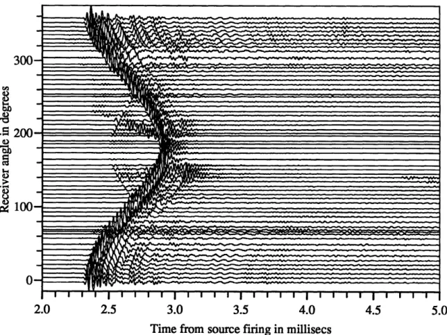
3-1 Raw data from the Complex shell. Incident angle = 900. Receivers 0°-360° by 6 ... 45

3-2 Raw data from the Complex shell. Incident angle = 90°. Receivers 00-3600 by 6. Each line scaled min to max. ... 46

3-3 Raw data from the Empty shell. Incident angle = 75°. Receivers 0° -3600 by 6. Each line scaled min to max ... 47

3-4 Raw data from the Ribbed shell. Incident angle = 75° . _Receivers -105°-750 by 3° . Each line scaled min to max ... 48

3-5 Raw data from the Complex shell. Incident angle = 75° . Receivers 00-360 by 6. Each line scaled min to max. ... 49

3-6 Raw data from the Complex shell. Incident angle = 660. Receivers

00-360° by 6. Each line scaled min to max. ... 50

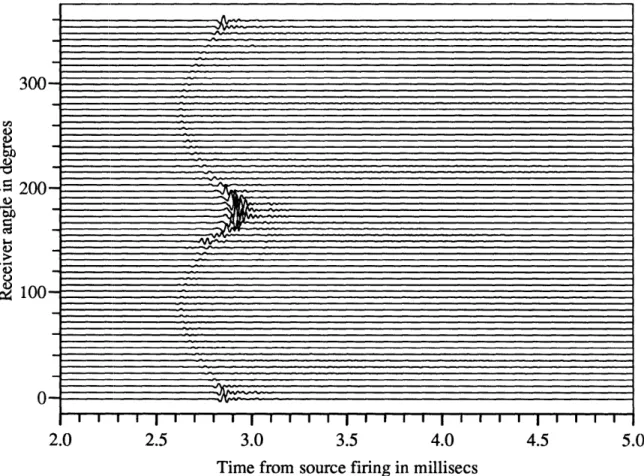
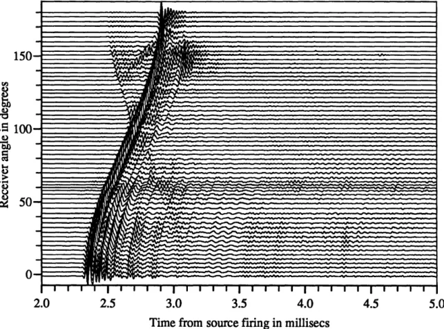
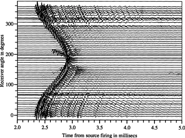
3-7 Raw data from the Empty shell. Incident angle = 0°_{. Receivers 0°-1800}

by 3 . _{Each line scaled min to max ... 52}

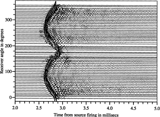
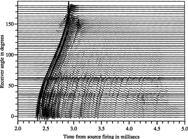
3-8 Raw data from the Ribbed shell. Incident angle = 0°_{. Receivers 0}°

-180° _{by 3}° . _{Each line scaled min to max ... 53}

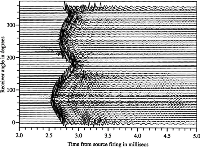
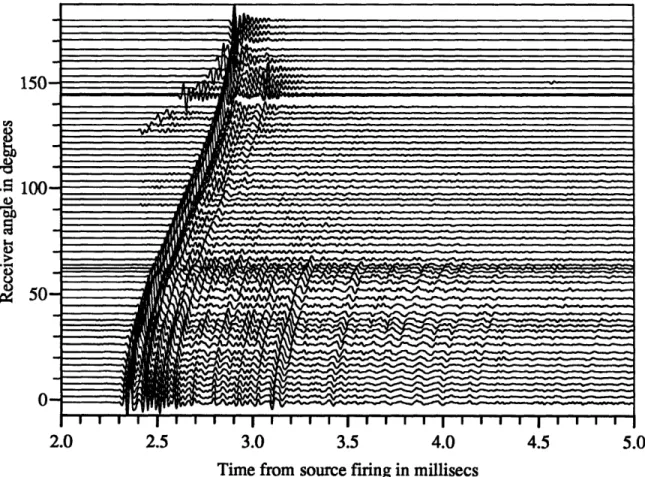
3-9 Raw data from the Complex shell. Incident angle = 0°_{. Receivers}

0°-180° by 3° . _{Each line scaled min to max. ... 54}

3-10 Raw data from the Empty shell. Incident angle = 5° . _{Receivers 0°-360}°

by 6. Each line scaled min to max ... 55 3-11 Raw data from the Complex shell. Incident angle = 5° . _Receivers

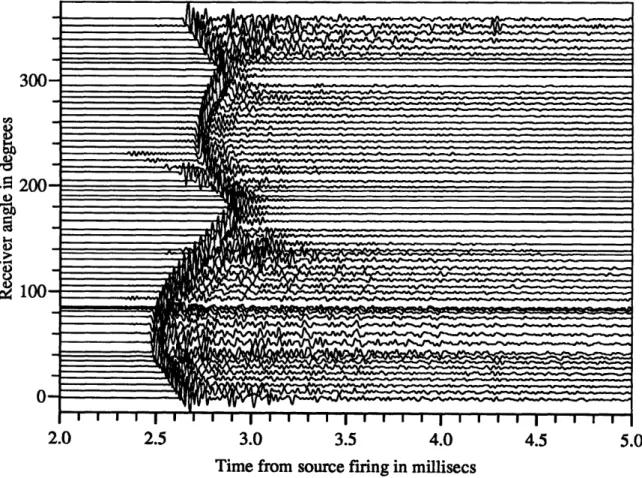
0°-360° by 6. Each line scaled min to max. ... 56 3-12 Raw data from 60° of the array by 1° _{around shell beam. Empty shell}

at 0° incidence ... 58 3-13 Raw data from 600 of the array by 1 around shell beam. Ribbed shell

at 0° incidence ... 59 3-14 (a) Source pulse and (b) Source spectrum. ... 60 3-15 (a) Hamming source pulse and (b) Hamming source spectrum ... 61 3-16 Raw data from 60° of the array by 1° _{around shell beam, deconvolved}

by source pulse. Empty shell at 0° _{incidence ... 62}

3-17 Raw data from 60° of the array by 1° around shell beam, deconvolved by source pulse. Ribbed shell at 0° incidence. ... 63 3-18 60° of array around shell beam, deconvolved by the source pulse and

focused onto shell. Empty shell data at 0° _{incidence. ... 65}

3-19 60° of array around shell beam, deconvolved by the source pulse and focused onto shell. Ribbed shell data at 0° incidence. ... 66 3-20 60° _{of array around shell beam, deconvolved by the source pulse,}

Ham-ming tapered and focused onto shell. Empty shell data at 0° _{incidence. 67} °

3-22 Block diagram of process used to remove geometrically scattered return. 69

3-23 Amplitude estimate for the geometrically scattered return from the

Empty (bold), Ribbed (plain) and Complex (dotted) shells at 0°

inci-dence ... 71

3-24 Amplitude estimate for the geometrically scattered return from the

Empty (bold), Ribbed (plain) and Complex (dotted) shells at 75°

in-cidence ... 72

3-25 Block diagram of complete direct analysis processing chain ... 73 3-26 60° of array around shell beam, geometrically scattered return removed,

deconvolved by the source pulse, Hamming tapered and focused onto shell. Empty shell data at 0° _{incidence ... 74}

3-27 60° of array around shell beam, geometrically scattered return removed, deconvolved by the source pulse, Hamming tapered and focused onto shell. Ribbed shell data at 0° incidence ... 75 3-28 60° of array around shell beam, geometrically scattered return removed,

deconvolved by the source pulse, Hamming tapered and focused onto shell. Complex shell data at 0° incidence ... 76 3-29 600 of array around shell beam, geometrically scattered return removed,

deconvolved by the source pulse, Hamming tapered and focused onto shell. Empty shell data at 5 incidence ... 78 3-30 600 of array around shell beam, geometrically scattered return removed,

deconvolved by the source pulse, Hamming tapered and focused onto shell. Complex shell data at 5 incidence ... 79 3-31 600 of array around shell beam, geometrically scattered return removed,

deconvolved by the source pulse, Hamming tapered and focused onto shell. Empty shell data at 750 incidence. ... 80 3-32 600 of array around shell beam, geometrically scattered return removed,

deconvolved by the source pulse, Hamming tapered and focused onto shell. Ribbed shell data at 75° _{incidence ... 81}

3-33 600 of array around shell beam, geometrically scattered return removed, deconvolved by the source pulse, Hamming tapered and focused onto shell. Complex shell data at 75° incidence ... 82 3-34 60° of array around shell beam, geometrically scattered return removed,

deconvolved by the source pulse, Hamming tapered and focused onto shell. Complex shell data at 660 incidence ... 83 3-35 60° _{of array around shell beam, geometrically scattered return removed,}

deconvolved by the source pulse, Hamming tapered and focused onto shell. Complex shell data at 900 incidence ... 84 3-36 Response of shell surface, energy integrated over space. Empty (bold),

Ribbed (plain) and Complex (dotted) shells for 0° _{incidence case. . . 87}

3-37 Response of shell surface, energy integrated over time. Empty (bold), Ribbed (plain) and Complex (dotted) shells for 0° _{incidence case. . . 88}

3-38 Response of shell surface, energy integrated over space. Empty (bold), Ribbed (plain) and Complex (dotted) shells for 750 incidence case. . . 89 3-39 Response of shell surface, energy integrated over time. Empty (bold),

Ribbed (plain) and Complex (dotted) shells for 750 incidence case. . . 90 3-40 Response of shell surface, energy integrated over space. Complex shell

at 66° _{incidence (bold) and Complex shell at 750 incidence (plain). . . 91}

3-41 Response of shell surface, energy integrated over time. Complex shell at 66° incidence (bold) and Complex shell at 750 incidence (plain). . . 92 3-42 600 of array around shell beam, geometrically scattered return removed,

deconvolved by the source pulse, and MLM focused onto shell. Ribbed shell data at 0° incidence. ... 93 3-43 Response of shell surface, energy integrated over time. Ribbed shell

for 0° incidence case, conventional (bold) and MLM focusing (plain). 94 3-44 Cramer-Rao bound estimate of resolution of source in presence of

sen-sor and line array noise. ... 97 3-45 Radon transform of waves traveling on the Empty shell using 0

inci-3-46 Radon transform of waves traveling on the Empty shell using 0°

inci-dence data. Isolated compressional slownesses ... 100

3-47 Magnitude of spectra of first forward and backward compressional waves. 101 3-48 Estimate of magnitude of compressional Reflection coefficient at stern endcap of Empty shell from 0° incidence data. ... 102

3-49 Radon transform of waves traveling on the Ribbed shell using 0° inci-dence data. . . . ... 104

3-50 Radon transform of waves traveling on the Complex shell using 900 incidence data. . . . ... .. . . 105

4-1 Forward modeling structure ... 108

4-2 Example of a transmission line model for the Empty shell . ... 111

4-3 Incident wave approaching an impedance. ... 115

4-4 Reflected, transmitted and coupled waves leaving an impedance .... 115

4-5 Example 1 of transmission line model. ... 116

4-6 Example 2 of transmission line model. ... 117

4-7 Example 3 of transmission line model. ... 118

4-8 Example 4 of transmission line model. ... 119

5-1 Focused Empty shell data used for match to Transmission line. Center of shell only, time traces de-weighted by average energy. . ... 127

5-2 Transmission line model for first compressional wave on Empty shell. 128 5-3 Transmission line model of first compressional wave on Empty shell.. 129

5-4 Transmission line model for reflected compressional waves on Empty shell ... 129

5-5 Transmission line model of reflected compressional waves on the Empty shell ... 131

5-6 Transmission line model for early-time flexural-induced compressional waves on the Empty shell ... 133

5-8 Transmission line model for late-time flexural-induced compressional waves on the Empty shell ... 136 5-9 Transmission line model of early and late time returns on the Empty

shell ... 137

5-10 Focused Empty shell data used for match to Transmission line. Center of shell only. ... 138 5-11 Transmission line model for the Ribbed shell. ... 139 5-12 Focused Ribbed shell data used for match to Transmission line. Center

of shell only. . . . ... 140

5-13 Transmission line model of the Ribbed shell ... 141 5-14 response of shell surface, energy integrated over space. Ribbed shell

for 0° incidence case, conventional (bold) and transmission line model

(plain) ... 142

5-15 response of shell surface, energy integrated over time. Ribbed shell for 0° incidence case, conventional (bold) and transmission line model

Chapter 1

Introduction

1.1 Motivation

Avoiding detection by adversaries has always been of great strategic military value. Accurate information about an enemy's position, strength and movement provides the key to the formulation of advantageous defensive and offensive maneuvers. For this reason, preventing the detection of one's own forces hampers an adversary's ability to make winning strategy. It also greatly enhances one's own by adding the element of surprise.

Technology has always played a vital role on both sides of the military long-range detection problem. As one side discovers a new detection technique, the other invents new countermeasures to defeat its advantage. In fact, since military technology among adversaries eventually equalizes through theft, copying, espionage, or purchase, the developer of such a technology also is forced to develop countermeasures to it in the eventuality that it will be used against him. For example, the engineers and scientists who developed Radar during WWII are the same people who later found that it was necessary to develop radar absorbent coatings and low cross section designs for their own aircraft in order to reduce their detectability by others with similar systems. This process continues in a never-ending upward spiral of technology, requiring detection and countermeasure systems of increasing complexity over time.

electro-magnetic radiation is completely absorbed by seawater within a few wave-lengths. This renders all radar, IR and visible systems useless for the detection of underwater vehicles. During WWI and II, German U-boats used this stealth capabil-ity to wreak havoc on British merchant ship supply lines [1]. Only the development of sonar detection systems was able to bring the threat under control.

The fact that only fairly low frequency sound waves are capable of long range prop-agation and the presence of many of its own and numerous adversaries' submarines in the worlds oceans have made acoustics of major importance to the US Navy. The drive by the US Navy to make its own vessels quieter was heightened particularly by the cold war with the USSR, when the mission of the ballistic missile submarine became to remain hidden near its target until such time as it might be needed. The fundamental principle which guides submarine design and operational strategy is that

the vulnerability of the submarine is directly proportional to its acoustic signature.

And so, there is a great deal of interest in the structural acoustic properties of ship and submarine hulls. To this end the Office of Naval Research is funding many efforts aimed at understanding the fundamental acoustic scattering processes of a submerged hull. Armed with such knowledge, designers can either avoid acoustically problematic structural arrangements or compensate for them.

For several reasons, this interest is currently focused in the mid-frequency range,

< ka < 10, where k = 2r/A, A is the acoustic wavelength in the water and a is

a characteristic length of the object. First, full scale test facilities exist and have provided empirical information about such structures in the low frequency, ka << 1, and high frequency, ka >> 1, ranges. Second, there is a great deal of theoretical support in these regimes: Raleigh and Born approximations [2] at low frequency and the Geometric Theory of Diffraction [3, 4] at high frequency. Finally, numerical meth-ods are computationally possible in these regimes. Thus, Finite Difference methmeth-ods have tractable grid sizes at low frequencies and Ray tracing becomes valid at high frequencies. All of this leaves a large gap in the understanding of these structures in the mid-frequency regime.

drical shells. The shells are thin, with thickness to radius ratios of typically 1%. They are constructed over bulkheads, rigid rib-like structures which support the thin hull membrane. They are further complicated by internal machinery and decks which are always resiliently mounted to the bulkheads. The internal structure to hull mass ratio is significant, on the order of 3 to 5 for typical submarine designs. Therefore, it is hypothesized that these discontinuities and mass loads will affect the acoustic properties of the vessel at mid-frequencies where wavelengths are on the order of the sizes of the the discontinuities.

In order to help the Navy understand the fundamental acoustic wave processes at work in a submarine hull at mid-frequency and to determine the effects of internal loading and hull discontinuities, the MIT Structural Acoustics Group has executed a number of mid-frequency, bistatic, scattering experiments on a set of model, finite, cylindrical shells. The simple shell models used in the experiments are not meant to mimic submarine design, but are designed in an incremental way to represent the fundamental acoustic components of the real structures.

The goal of this thesis is to extract information about these structural acoustic wave processes from the experimental data. The important parameters of these pro-cesses include wavespeeds, dispersion relations, decay rates and reflection, transmis-sion and wave coupling coefficients at discontinuities. Measurements in the scattered acoustic field of these models contain much of this information. However, it is buried in the complex interaction occurring between the fluid and structure, including the propagation path to the measurement system. The sound field at the collection array therefore must be decomposed into fundamental, understandable pieces, via array processing, signal processing and forward modeling. This task is complicated by the mid-frequency nature of the data where both time and frequency resolution are poor.

1.2 Previous Research

The set of shells described in this paper was first investigated in backscatter from a previous set of monostatic experiments. The interesting incident angles where

quasi-longitudinal and quasi-shear waves couple onto the shell through phase matching were identified by Corrado [5]. His preliminary studies provided basic knowledge which guided my further investigation of membrane waves on the shell. In addition, he identified helical shear waves as the major contribution to the backscattered field near beam incidence. At the writing of this thesis, another set of experiments is being conducted by MIT to investigate the damping of these waves by sandwiching

a visco-elastic layer between two structural layers.

Mackovjac [6] processed the bistatic experimental data with Maximum Likelihood beamforming to identify structural resonances in the data. His processing is limited to the late-time portion of the data and a plane wave approximation. The resolutions he attains can be understood in the light of the Cramer-Rao bounds calculations done in Section 3.7 of this thesis.

Acoustic holography has been done on a much simpler set of Empty shells pro-viding both pressure and velocity measurements on the surface of the shells [7-i 8]. Results from these experiments show the same types of features that are observed in our Empty shell.

The effect of internal loading on the scattering from infinite shells has been studied analytically by Achenbach [9] and Guo [10] and has been found to be significant. In

particular, the location of attachment and the nature of the attachment, pinned

versus rigid, has been shown to greatly affect the scattered field due to interaction with structural resonances of the shell.

Finally, Ricks [11], also of the MIT Structural Acoustics Group, has a numerical, full-elastic layered, cylinder model which is capable of computing the response of infinite cylinders to ring forces. Ricks is also investigating the effects of including a flat plate bulkhead and may be able to provide a benchmark for the results in this thesis in the near future [12].

1.3 Hybrid Processing Approach

There are many possible approaches which can be used to analyze a large experimental dataset such as the one described in this thesis. However, most processing tends to fall into one of two broad categories, either direct analysis or forward modeling. Each of these two approaches implies a specific processing structure and a set of advantages and disadvantages.

The structure of what can be called the direct analysis method is shown in Fig. 1-1.

In this approach, the experimental data is considered to be the input to the processing

chain. Direct analysis is then used to extract estimates of the physical variables of interest, which are the output of the processing chain. Examples of methods which fall into this category include beamforming, spectral analysis and linear filtering.

Data

Direct

hIysical

|At

Array

Analysis

'I Variables

Figure 1-1: Direct analysis approach.

There are many advantages to this type of approach. The analysis is usually sim-ple, analytically tractable and computationally efficient. It is also generally performed only once on a dataset, such as an FFT to determine spectral content. There are a large number of direct analysis methods to chose from, each complete with sizable body of literature.

However, there are several disadvantages to this type of approach. Generally, the accuracy of the physical variable estimates is limited by some parameter of the data collection, such as resolution of the measurement array, the sampling rate, data quan-tization or the signal to noise ratio (SNR). These methods, usually data transforms, are subject to processing artifacts. Aliasing, sidelobes and other process-introduced signals often contaminate results. And finally, even if these processing concerns are adequately addressed, the results given by such processing usually are not expressed in terms of the physical variables of interest. For example, a spectral analysis of the acoustic field received at a hydrophone array will quantify the energy present

at a particular frequency, but cannot separate, say, the amplitudes of forward and backward traveling waves.

The structure of the forward modeling or matched-field approach is shown in Fig. 1-2. In this case, estimates of the physical variables of interest are used as the inputs

to a model which outputs synthetic data. Then the estimates and the model are

ad-justed until the synthetic data matches the collected data. Finite Element, Boundary

Element and Wavenumber Integral modeling all fall into this category.

Physical

I

Forward

Data

Variables

'

Modeling

i

At Array

One advantage of this approach is that it is not limited by the parameters of the data collection. Since models are defined exactly, the model output can in theory be calculated to essentially "infinite" resolution and precision. Also, unlike direct analysis, by tracing the answers back through the model, it is usually possible to

understand the fundamental parameters of interest. In fact, this technique is often

used when both the input and the output are known. For example, in long-range ocean propagation problem, the input source characteristics are simple but the ray paths are of interest. If the input is not known, the method is even more valuable. Once a good match is made, the process provides both an estimate of the physical parameters and a model of the system being studied. Once this model is identified, the user can then explore it with new parameters to investigate similar problems. Use of this method is also valid when the actual system is too complex to model completely, the major contributions can be modeled and major features only matched. This allows partial understanding of complicated systems.

This structure too has its limitations. Unlike the direct analysis approach, this process is generally repeated many times either by hand or automatically using a feedback loop to adjust the parameters based on the data match. This can take

generally available in computer libraries and usable in very generic forms, forward modeling usually requires a good deal of hand coding to match specific problems. High model complexity is often required to match even the coarsest features of real data. The complexity of the model is often several orders of magnitude greater than the direct analysis approach and these more complicated schemes have a tendency to-wards numerical instability and other unidentifiable artifacts. In addition, the model required is sometimes too complicated to compute. Current Finite and Boundary El-ement methods require more computing power than is currently available to compute even canonical problems, much simpler than the complicated geometries like those present in the experiments described in this thesis. Finally, it is often necessary to model many "uninteresting" processes in order to match the data, particularly if the "uninteresting" processes dominate. For example, it would be necessary for a Finite Element code to model the propagation path from the shell to the collection array, even though that path is well understood. This is not an interesting part of the prob-lem, but it must be included in the model for the data to match at all. These kinds of issues greatly increase the model complexity.

Notice that the advantages and disadvantages of these two types of approaches are for the most part non-overlapping. This suggested a hybrid approach to me. Ideally, it would be best to take advantage of only the favorable characteristics of each of these types of methods and avoid the problematic characteristics completely. This is of course impossible in practice. However, it is possible to use one approach for that part of the processing where its strong characteristics produce the most benefit and switch to the other approach when the first approach begins to have problems. In this case, the approach should use low resolution direct analysis to eliminate the "uninteresting" features of the data and then use forward modeling to model only the interesting features at high resolution. A block diagram of the Hybrid Processing Structure which accomplishes this goal is shown in Fig. 1-3.

I have chosen the waves traveling on the shell as the center of the Hybrid Pro-cessing Structure. It is the output of both the direct analysis and forward modeling and is therefore common to both legs. I have chosen this space as the central output,

Physical

Variables

I

4

Direct

s

Data

Analysis

On Shell

Figure 1-3: Hybrid approach

because it is an intuitive space in which to think about the fundamental physical

processes at work on the shell. Waves traveling on the shell can be interpreted qual-itatively after the direct analysis. Then the modeling can be used to complete those interpretations and quantify physical variables of interest.

There are several benefits to this processing structure in addition to the benefits

listed above for each leg. The model used in the forward modeling leg can be simple and readily computable because the direct analysis eliminates the "uninteresting" features which complicate modeling. The low resolution of the direct analysis now does not limit the estimation of the physical variables of interest as it has been decoupled from the problem by the forward modeling. This hybrid structure removes the major obstacles posed by either approach alone.

This Hybrid Processing Structure is the major contribution of this thesis. Note that this is not a traditional analysis/synthesis approach. That type of approach is embodied in the forward modeling leg alone. The direct analysis leg has supplemented that traditional approach and increased its robustness for solution.

1.4 Organization of Thesis

This chapter has provided some motivation for this thesis, background information on the problem and an outline of my basic processing approach. The remainder of this document outlines the details of the approach and presents the results obtained

Data

At Array

Forward

Chapter 2 describes the various array processing methods used to implement the direct analysis leg of the Hybrid Processing Structure. This chapter begins with a description of the three shell designs, followed by a description of the experimental geometry, which will motivate the need for array processing. Section 2.2 continues with the description of the conventional beamformer which lays out the terminology and the theoretical framework for the non-adaptive, conventional focusing method in Section 2.3, the major processing tool of this direct processing step. An adaptive beamformer, the Maximum Likelihood Method, is also briefly formulated in Section 2.4 for later comparison and computation of resolution limitations. Additional direct processing, the Radon Transform, is described in Section 2.5. The Radon transform is a generalized 2-D Fourier transform used in the Seismic community. It is useful in this context for separating wavetypes.

Chapter 3 illustrates the results obtained with the various direct methods

de-scribed in Chapter 2. The raw data from the shell is presented in Section 3.1 to indicate the problem at hand. The methods of Chapter 2 are applied to the data to yield the components of the dynamic structural response of the shell which are ob-servable at the array. These methods are aided by source pulse deconvolution, array weighting and removal of the geometrically scattered return. These are described in Sections 3.2, 3.3 and 3.4. The resulting processed data clearly shows the radiating waves traveling on the shells. The complete processing chain is applied to all available data and presented in Section 3.5 along with a discussion of the major features of each dataset. The locations of discontinuities and their effects on the partitioning of energy within the shell bays is shown via the integration of energy along the time and spatial axes of the data in Section 3.6. The discontinuities in the shells give rise to reflections and transmissions that can be seen but not quantified due to the

limits of the data time and spatial resolution. The resolution limit of the

process-ing is quantified via comparison with the Maximum Likelihood beamformer and the Cramer-Rao bounds of the focusing process in Section 3.7. Comparison of this result with the integrated energy representation shows a discrepancy between actual and theoretical resolution which is later resolved via forward modeling. Finally, a crude

estimation of the Reflection coefficient for compressional waves at the endcap in the Empty shell is made using the Radon Transform in Section 3.8. The poor quality of this estimate typifies the use of the direct approach alone to solve this type of problem and motivates the need for forward modeling.

Chapter 4 describes the models and parameter estimation methods used to im-plement the forward modeling leg of the Hybrid Processing Structure and circumvent

the resolution limitations. The general structure of the parameter estimation process

is discussed in Section 4.1. It mainly consists of a model and a parameter adjustment process. Section 4.2 describes the motivation for and the details of the Transmission Line model used to represent the shell. Several examples of the capabilities of this model are included. Finally, Section 4.3 describes the Simulated Annealing method

used to adjust the parameters of the model to match the data.

The transmission line model described in Chapter 4 is used in Chapter 5 to match the focused data computed in Chapter 3 for the 0° incidence case. This is accom-plished through a step-by-step process which slowly increases the complexity of the model. Section 5.1 matches the parameters which pertain to the compressional waves traveling on the Empty shell. Sections 5.2 and 5.3 describes the models used to match the early and late time flexural-induced returns respectively. Finally, Section 5.4 shows the model used to match the data from the Ribbed shell at 0° _incidence.

The integrated energy plots for this case clear up the discrepancy between observed and theoretical resolution brought up in Section 3.7.

Chapter 6 provides a summary of the major results of the thesis and recommen-dations for future work.

Chapter 2

Array Processing

2.1 Motivation

Sound is intrinsically four dimensional. The signals that our ears receive vary as we move about space in three dimensions and as time passes. Both the time and spatial

structure of a sound field carry a great deal of information. For example, if we were to record the electrical output from a single microphone in a room over time, we could tell from the spectrum of the signal if there were a periodic source present, such as a motor, a speaker, the gender of that speaker, the noise level etc. Spatial processing is equally powerful. This is evidenced by the fact that with only two array elements, our ears, sampling the sound field at only two points, we are able to localize a speaker in a room quite accurately. The same characteristics of sound that allow a person to focus on a speaker's location are the same characteristics that allow array processing to isolate sources of sound to different parts of the shell. This information is basically carried in the arrival time of a signal at an array element.

Array Processing is the spatial equivalent to Digital Signal Processing (DSP) in time as they both involve sampling a continuous process. DSP requires time sampling of signals and provides the mathematical formalism for frequency filtering operations. Array processing requires spatial sampling of the field and provides the mathematical formalism for spatial filtering operations. This formalism is identical for signal and array processing and in fact there would be no difference in their analysis if it were

not for the physical limitations of arrays. The advent of computers has brought DSP to the forefront of signal analysis [13], since algorithms for processing digital signals only require software rather than an additional hardware investment as do analog algorithms. The hardware for time sampling of analog signals is fairly easy to acquire and once it is set up, an essentially infinite digital time series can be collected. The application of array processing mainly suffers from the constraints of the analog data acquisition part of the problem, since an additional physical sensor in general is required for each additional spatial sample. Because array elements are expensive and hard to place, arrays are often of limited lengths with few samples; often the sensors are not even equally spaced. This is in contrast to time sampling which has a large body of literature dedicated to processing of long, equally spaced digital time records. And finally, array processing is often complicated by the fact that arrays often sample over 2 and 3 spatial dimensions. In most cases, these differences between time and spatial sampling require that novel approaches to array processing be devised.

This chapter describes the array processing techniques used to implement the direct analysis leg of the Hybrid Processing Structure described in Section 1.3. The need for array processing is motivated by the data collected in the bistatic scattering experiments. Section 2.1.1 provides a description of the three model shells used in the experiments and Section 2.1.2 describes the experimental geometry used to measure the acoustic scattered field from these shells.

Section 2.2 describes the conventional plane-wave beamformer, the basic and most general array processing operation, and provides a notational basis for the remainder of the chapter. This general processing structure is then specified to conventional focusing in Section 2.3, which is the major tool of direct analysis used in this thesis. Both the conventional beamforming and focusing are non-adaptive approaches to array processing as neither takes into account any information about the structure of the field to reduce ambiguities. An adaptive approach known as the Maximum Likelihood Method (MLM) which uses the cross correlation of the field between array elements as a priori information to optimize array response, is derived briefly in

direct processing in Chapter 3 using the Cramer-Rao bounds. Finally a description of the Radon Transform is presented in Section 2.5. This will be used to separate forward and backward traveling waves on the shell to estimate reflection coefficients in Chapter 3.

2.1.1

Model Designs

The MIT Structural Acoustic Group effort is concentrated on a number of experiments conducted on three, 90:1 scale submarine models designed by Conti and Dyer [14] and built by the Naval Research Laboratory (NRL) to high tolerance. These shells are the source of all the acoustic phenomenon described in this thesis.

The first model is a finite, thin, air-filled, cylindrical shell constructed from a nickel alloy, Ni-200. The ends of the shell are closed with a spherical endcap connected to the shell by a short conical section. A mechanical drawing of this shell is shown to scale in Fig. 2-1. The model has Thickness to Radius Ratio, t/a = 0.96%, Aspect Ratio, L/2a = 7.75 and Ring Frequency, frin = 14kHz. This model is designated

the Empty shell throughout this thesis.

f-"

33.93"

---44~

~29.09"

4%d

.

Figure 2-1: Empty shell design.

The second model is identical to the Empty shell except for the presence of four, massive, internal, nickel ring stiffeners welded to the shell. The total mass of the four rings is equal to the mass of the shell. These stiffeners are irregularly spaced and shown to scale in Fig. 2-2. This design was chosen over one with equally spaced ribs to eliminate ambiguities in the sound field due to structural periodicity. This model is designated the Ribbed shell throughout this thesis.

quadrant-Stem

Figure 2-2: Ribbed shell design.

symmetric, resiliently-mounted, wave-bearing, internal structures. Four stainless steel masses are independently mounted to each ring stiffener with triangular blocks of EAR C1002 Isodamp rubber. An epoxy compound connects the rubber to the rings. A detailed drawing of the ring mounting is shown in Fig. 2-3. Corresponding masses

Drill

Figure 2-3: Ring and suspended mass system in the Complex shell.

in each ring are connected by Delrin rods, which have a measured quasi-longitudinal wave speed of cl t 1625m/s. This arrangement allows waves to travel between the rings internally and is meant to simulate the low wavespeed paths in an actual submarine through machinery and decks. A typical pair of connected ribs is illustrated in Fig. 2-4. The ratio of the total mass of all rings and internals to the mass of the shell is approximately 3, which is typical for submarine designs. The system of the rubber and the suspended masses were designed to have a natural frequency less than 1/3 the ring frequency of the shell. This design is designated the Complex shell

Figure 2-4: Wave-bearing system in the Complex shell.

2.1.2

Experiment

The NRL Building 71 Scattering Measurement tank was used to acquire all data. The geometry of all experiments discussed in this thesis is shown in Fig. 2-5. The submerged shell was ensonified by a line array source 3m in length at a distance of 2.18m from the target center. The elements of the line array source were shaded to provide a plane wavefront incident at the shell. The source pulse was a wideband pulse with fairly uniform response from 10khz < f < 50khz. This pulse is described in greater detail in Section 3.2. The shell could be rotated in plane with respect to the source array to provide different angles of incidence. Bistatic data was collected for incident angles of Oi = 0°_{, 66}°_{, 75}° _{and 90}° _{for reasons to be discussed in Section}

3.1.1.

A single receiver was rotated 3600 azimuthally around the shell in plane with the shell center and source array at a distance of 2m from the target center. Time records were recorded at 1 degree increments, providing a synthetic array measurement. The data was sampled at 500khz, oversampled by a factor of approximately 5. 4096 time samples were collected after an approximately 2msec delay following the source firing. To reduce the contribution of incoherent signal components, 100 such time series were collected at each location and averaged. All measurements were calibrated and converted from receiver voltage levels into units of pressure (Pa).

The measurement of the scattered field from the target was computed in the

60°Sub-array 0.18 m I, 90 '- %_ I I _I %_%

Synthetic

,

Figure 2-5: Experimental geometry.

first with the target in place and then with the target removed. This latter dataset provided a measurement of the tank clutter and the direct field from the source. It was subtracted from the former total field to form the scattered field measurement. Finally, a rectangular window with Hamming ends was applied to the time record to zero out target-dependent returns from the tank walls, floor and the water surface. Clutter subtraction is the limiting noise process, the SNR following this process is ap-proximately 30dB. An ambient noise measurement shows that the background noise spectral level is 50dB down from the signal level. Further details of data acquisition can be found in Corrado[5].

2.2 Conventional Beamforming

In order to understand the formulation of the conventional focusing algorithm and later the MLM algorithm, it is useful to develop some notation and the structure of the conventional beamformer. Since all the elements of the scattering experiment are in-plane with respect to one another, I will restrict my discussion to two dimensions

In all experiments, the target, source and collection array are submerged in water, a homogeneous medium which supports no shear stresses. The pressure field, P, in this medium satisfies the homogeneous wave equation:

P - c0V2P = O (2.1)

dt2

where V2 in this case is the two-dimensional gradient operator and co is the sound-speed in the water. Plane waves are one solution to this equation [2]. A single plane

wave is defined as:

s(t, r),k = S(w, k)ej(wt-k r) (2.2)

where the pressure field, s, is a function of time, t, and a position vector, r, at every an-gular frequency, w, and wavenumber, k. In a simple x - y cartesian coordinate system,

the wavenumber vector is derived from the wavenumber as, k = (IklcosO x, IklsinO y), where 0 is the angle of arrival of the plane wave. In general, the spectral level, S of the plane wave is dependent both on frequency and wavenumber.

The relationship between the angular frequency, w, and the wavenumber, k, is set by a propagation constraint from the governing wave equation for the medium. For homogeneous water, as in the experiment, the compressional soundspeed, co is assumed to be constant over space and time. In this case, Eq. (2.2) is a solution to the wave equation if the wavenumber satisfies the dispersion relation:

k = 2r/ = w/co (2.3)

where A is the wavelength. Such a medium is known as non-dispersive. All frequencies travel at the same soundspeed so that energy packets traveling in the medium do not spread out over time. Later, this will not be the case for structural waves traveling on the shells.

The block diagram of the structure for a conventional beamformer is shown in Fig. 2-6. A field s(t, r) impinges on a space populated with N receiver elements at positions z,. Time series, xn(t), are collected at each receiver position and fed into

'Xl(t) G (c)

,x2(t) G20) I

s(t, r) zY -- y (t)

Figure 2-6: General beamforming structure

filters, G,(w), which generally consist of an amplitude weighting and a time delay. The outputs of these filters are added together to provide the output, y(t). The output is determined by the characteristics of the filter components and the incoming field. Array processing which fits in to this structure is known as "delay and sum" beamforming.

Any signal, s(t, r) can be broken down into a set of orthogonal basis functions in a plane-wave decomposition as follows:

s(t, r)

k

S(w,

(2.4)

where D is the spatial dimensionality, in my case 2. Therefore, y(t) can be determined for each w and k, i.e. we can determine the response of the beamformer to each plane-wave, then the results are superposed for the final answer.

The output of the conventional plane-wave beamformer to a single unit-amplitude plane wave would be:

N

Y(t)l,,k = E Gn(w)ejwte- ikTzn = Et(k)G(w)e j t (2.5)

where: E(k) = ejkTzl eJkTz2 ejkTzN

,G(w) =

and t indicates conjugate transpose.

Et(k)G(w)ejwt is known as the array response function, because it determines how the array will respond to incoming plane waves from various directions. G(w) is called the weight vector. This weighting is generally adjusted to decrease the sidelobes of the array response function. E(k) is known as the steering vector, since adjustment

to the exponential modulation results in an adjustment of the major response axis of

the array. The direction of maximal array response can be steered by offsetting the wavenumber in the steering vector. When the array is steered to wavenumber kt, the response becomes:

y(t)[I,k,kt = Et(k - kt)G(w)ejwt _(2.7)

In this case, if an incoming plane wave, s(t,r)IW,kt = S(w,kt)eJ(wt-kt T r), impinges

on the receivers and the weighting vector is normalized such that, 7N=l Gn(w) = 1,

then the output y(t)l, = S(w, kt)ej"_{t, which is a unbiased estimate of the input. This}

phase delay is usually implemented by a delay in the filters, Gn(w), but notice that

it is mathematically incorporated into the steering vector, E(k) rather than in the

weighting vector, G(w).

This formulation works for a plane-wave decomposition of the field. For any fre-quency, the output of this type of beamformer is generally a signal or signal power as a function of arrival angle. This angle is appropriate for truly plane waves. The plane wave assumption is valid in the far field of an object where the spherical wave-fronts are of such large radius of curvature that they are essentially plane. However,

the experimental data under consideration in this thesis were measured in the near

field of the shells. Here the plane wave assumption is not a good one. The next section describes the conventional beamformer modified to eliminate this plane wave assumption.

2.3

Conventional Focusing

The purpose of the direct analysis leg of the Hybrid Processing Structure described in Section 1.3 is to understand the waves traveling on the shell itself which, over time, re-radiate substantially through a large angular region. To do this, it is only necessary to remove the delay and superposition effects of the propagation path from the shell surface to the receivers. This will allow direct observation of the dynamic response of the surface of the shell which is capable of radiating into the far field.

Fortunately, the plane wave assumption is not appropriate at this particular

mea-surement radius. If the meamea-surements had actually been made in the far field, all the phase information in the field which allows spatial separation would have been lost. At beam aspect for this target, the near field range, defined by L2/A, is approx-imately 13m at mid-band. The receivers, located at 2m from the target center at beam, are therefore well within the nearfield of this shell as a whole. As a result, the field measured at the receivers contains phase information which allows the response of different parts of the shell to be separated.

At this point, a model for the field must be chosen. Many different models are possible. However, the idea is to choose a simple model which will be computationally tractable. Ideally, the best model would be one which includes all the traveling waves on the shell, radiation of these waves and propagation to the collection array. This would require matching the data generated by the forward model to data collected at the array which not only defeats the purpose of the Hybrid Processing Structure but would most likely be computationally impossible. Therefore, a simple model is chosen here and later its resolution will be computed using the Cramer-Rao bounds of an optimal processor, the MLM.

Backpropagation requires coherent addition of the receiver elements for each po-sition on the shell, also known as conventional focusing. The field is assumed to be generated by a finite number of virtual, point sources at points z'i on the shell with

time response si(t). The data seen at the nth receiver, located at Zn is then given by:

(2.8)

1 )_(

X.(t)

=

E

4

rd,

Si

where d,,i = jz'i - z,n and co is the soundspeed in the water.

Each source signal can be reconstructed by combining the response from each of the receiver elements as depicted in Fig. 2-7. In the time domain, this conventional

z2

z3 _z

4

Z' z

Figure 2-7: Intuitive focusing operation

focusing operation is defined:

yi(t) = E 4 dmiXn t + i Gn(W)

n=1 CO

(2.9)

where, as before, Gn(w) is a weighting coefficient on each receiver to be used later in sidelobe reduction. yi(t) provides an estimate of the source response, si(t). To see this, substitute the expression for x,(t) into Eq. 2.9:

yj(t) = E E dsi t Gn(w)

n=l ,i

co

If nE=1 Gn(w) = 1 and si(t) = 0 for i j, then yi(t) = s(t). Since more than

contaminated by the response from other points. The degree of contamination is determined by the resolution and sidelobe structure of the collection array.

A synthetic example of the results of this kind of focusing is shown in Fig. 2-8. Here the impulses from three sources overlap across the array. Focusing will constructively

add the channels to synthesize the response from each source. This is an idealized example, in reality there would be sidelobes from the processing.

I I I I I I I I I I I I I I I I I I I I I I I II I II I a I I I I I I I I t x I I I I I I

Figure 2-8: Synthetic focusing example

The formulation of conventional focusing can also be expressed in terms similar to the conventional beamformer. To see this, consider the response of a system which is focused at source j measuring the field from source i:

N

-

)

ybi -=

Z

, Sit -

G.,(w)

or in the frequency domain:

y(t)lii= E d S(,()ejWte-Jk(dni-dn )Gn(W)

Et(d,j

-n=l n," dn,i)G(w)ejt (2.12) where:

E(d,j - dn,) =

, G(w) =

This mathematical structure carries over to the MLM formulation in the next

section.

2.4 MLM Focusing

The beamformers described in the last two sections are non-adaptive in nature. By this, I mean that the weight vector, G(w) is fixed. However, this type of filtering is sub-optimal in a probabilistic sense, as it does not use the available a priori knowledge about the incoming signal to reduce sidelobes and improve the output response. A class of beamformers which does utilize this information are called adaptive. These filters generally require an the incoming signal covariance across the array.

One such adaptive beamformer is the Maximum-Likelihood Method (MLM). This "high resolution" beamformer has been studied in detail [15, 16, 17, 18] mainly be-cause of its analytical tractability and bebe-cause it can be shown that if there is an "optimal" solution to a problem, one which uses all a priori information, that so-lution is the Maximum Likelihood soso-lution [19]. This beamformer will be used in Chapter 3 to show estimate the spatial resolution of the direct analysis. The concept behind this processor is quite simple. The first characteristic that is desirable for

any beamformer is that the output is normalized to maintain energy in the target

direction. In the matrix notation of the last two sections, this is expressed:

Et(kt)G(wlkt) = 1 (2.14)

With this constraint in force, the output energy of the beamformer must be min-imized:

min SY(w) (2.15)

G(w)

where S(w) = Gt(wlkt)K,(w)G(wkt) and K,(w) is the actual input covariance

matrix across the array.

The weight vector which satisfies these requirements is simply:

K-l(w)E(kt)

G(wlkt) = (2.16)

Et(kt)K-l(w)E(kt) (2.16)

The MLM beamformer uses the information in the field to adjust the weight vector such that signals from any direction other than the a priori signal direction are rejected. This improves the sidelobe response of the beamformer and greatly sharpens the mainlobe as well.

For stationary, homogeneous processes the covariance matrix is given by:

K,(w) = X(w)Xt(w) (2.17)

where X(w) = (Xi(w),X 2((w),..., XN(W))T, the Fourier coefficient of the time series

at each receiver. However in practice, the input correlation matrix must be computed

with extreme care. The assumption made in this derivation is that the input signal is

stationary and homogeneous. The wave components propagating on the shell generate arrivals at the receiving array which are transient and inhomogeneous. Therefore, it is necessary for this analysis to be performed over short time intervals. Time windowing of the input signals is used to accomplish this.

Since the time response of each array element must be windowed, it is necessary

to compensate for the delays to the sensors. Otherwise, the windowing operation in the covariance matrix computation will exclude the actual time of interest. In

a plane-wave formulation, the delays are simple stacking operations, see [20, 21] for details. In the case of focusing however, the stacking operation must be replaced with a focusing operation. Notice that the same model is being used in this beamformer as in the conventional focusing operation. This will be important in the resolution

computation.