An Analysis of Profit Cycles In the Airline Industry

MIT

MIT

ICAT

ICAT

MIT International Center for Air Transportation

An Analysis of Profit Cycles

In the Airline Industry

By

Helen Hong Jiang and R. John Hansman

Report No. ICAT-2004-7

December 2004

Massachusetts Institute of Technology

Cambridge, MA

An Analysis of Profit Cycles in the Airline Industry

by

Helen Hong Jiang and R. John Hansman

ABSTRACT

The objective of this paper is to understand the financial dynamics of the airline industry by identifying profit cycle periods of the industry and their driving factors.

Assuming that the industry profit cycles could be modeled as an undamped second-order system, the fundamental cycle period was identified to be 11.3 years for the U.S. airlines and 10.5 years for the world airlines. Analyses of industry profits reveal that such cycle period is endogenous, neither deregulation nor September 11 have significantly changed it.

Parametric models were developed under the hypothesis that phase lag in the system caused profit oscillations; and two hypotheses, lag in capacity response and lag in cost adjustment were studied. A parametric model was developed by hypothesizing the delay in capacity response caused profit oscillations. For this model, the system stability depends on the delay between aircraft orders and deliveries and the aggressiveness in airplane ordering. Assuming industry profits correlated to capacity shortfall, the delay and gain were calculated and the results were consistent with the observed delay between world aircraft deliveries and net profits. Since the gain in the model has lumped impacts of exogenous factors, exaggerated capacity response was observed in simulation. This indicates capacity shortfall alone cannot fully explain the industry dynamics. The model also indicates reduced delay may help to mitigate system oscillations. Similarly, a parametric model was developed by hypothesizing the delay in cost adjustment caused profit oscillations, and simulation results were consistent with industry profits. A coupled model was developed to study the joint effects of capacity and cost. Simulations indicated that the coupled model explained industry dynamics better than the individual capacity or cost models, indicating that the system behavior is driven by the joint effects of capacity response and cost adjustment. A more sophisticated model including load factor and short-term capacity effects is proposed for future work in an effort to better understand the industry dynamics.

This document is based on the thesis of Helen Hong Jiang submitted to the Department of Aeronautics and Astronautics at the Massachusetts Institute of Technology in partial fulfillment of the requirements for the degree of Master of Science in Aeronautics and Astronautics.

ACKNOWLEDGEMENTS

The authors would like to acknowledge the R. Dixon Speas Fellowship, the MIT Global Airline Industry Program and the Alfred P. Sloan Foundation in supporting this research.

The authors would also like to acknowledge Dr. Peter Belobaba and Professor Steven R. Hall of MIT, Mr. Drew Magill and Dr. William Swan of Boeing Commercial Airplanes, Dr. Christoph Klingenberg and Dr. Alexander Zock of Lufthansa German Airlines, Mr. Stephen K. Welman of The MITRE Corporation, Dr. David W. Peterson of Ventana Systems, Inc., and Professor James M. Lyneis of Worcester Polytechnic Institute for valuable suggestions and feedbacks.

Thanks to Diana Dorinson, Thomas Gorin, Bruno Miller, Liling Ren, Ryan Tam, Emmanuel Carrier, and Phillippe Bonnefoy in the MIT International Center for Air Transportation for valuable discussions related to this research.

TABLE OF CONTENTS

CHAPTER 2: Methodology for Airline Net Profit Analysis……….. 23

2.1 Assumption and Derivation of Airline Net Profit Model………...………... 23

2.2 Identifying Fundamental Cycle Period of Airline Industry………... 24

2.3 Model Estimation….……….. 27

CHAPTER 3: Results of Airline Net Profits Analysis………. 29

3.1 U.S. Airline Industry before Deregulation……… 29

3.2 U.S. Airline Industry after Deregulation………... 31

3.2.1 Impact of Deregulation on Profit Cyclicality………... 31

3.2.2 Impact of September 11 on Profit Cyclicality………. 32

3.3 World Airline Industry……….…. 34

3.4 Assumptions and Limitations of Airline Net Profit Model……….….. 34

3.5 Summary of Airline Net Profit Analysis………... 35

CHAPTER 4: Parametric Model for Capacity……….... 37

4.1 Data Analysis of World Commercial Jet Orders and Deliveries………... 37

4.2 Capacity Hypothesis……….. 40

4.3 Parametric Model for Capacity………. 41

4.4 Root Locus Analysis of System Stability……….. 42

4.5 Determining Parameters in the Capacity Parametric Model………. 44

4.5.1 Assumptions………. 44

4.5.2 Derivation……… 45

4.5.3 Parameters for the Airline Industry……….. 46

4.6 Factors Contributing to Delay and Gain Values……….... 47

CHAPTER 5: Simulations of Capacity Parametric Model……… 49

5.1 Capacity Simulations of the U.S. Airlines………. 49

5.2 Revisiting the Assumption – Cost of Adding Capacity………. 51

5.3 Capacity Simulations of the World Airlines……….. 51

5.4 Mitigating System Oscillations……….. 53

CHAPTER 6: Parametric Model for Cost………... 57

6.1 Cost Hypothesis………. 57

6.2 Parametric Model for Cost………. 59

6.3 Unit Net Profit Analysis……… 60

6.4 Determining Parameters in the Cost Parametric Model……….... 61

6.5 Simulation Results……….……….... 62

6.6 Summary of Cost Parametric Model………. 65

CHAPTER 7: Coupling Capacity and Cost Effects……… 67

7.1 Coupled Model Combining Capacity and Cost Effects………. 67

7.2 Parameter Values in the Coupled Model………... 69

7.3 Simulation Results………. 72

7.3.1 Simulation 1 – Calibration Simulation………. 72

7.3.2 Simulation 2………. 77

7.3.3 Simulation 3………. 82

7.4 Summary of Coupled Model……….… 86

CHAPTER 8: Including Load Factor and Short-term Capacity Effects……….. 87

8.1 Model Including Load Factor and Short-term Effects.………. 87

8.2 Demand Modeling………. 88

8.2.1 Latent Demand Concept……….. 88

8.2.2 Demand Models……….………….. 89

8.3 Revenue Management……….….. 90

8.4 Capacity Modeling………. 91

8.4.1 Two Capacity Concepts………... 91

8.4.2 Tactical Scheduling Model……….………. 92

8.4.3 Fleet Planning Model……….……….. 93

8.5 Modeling Cost Factors……….. 93

8.6 Summary..……….………... 94

CHAPTER 9: Conclusions...………. 95

9.1 Summary of Findings……… 95

REFERENCES……… 97

APPENDIX A: Average Aircraft Utility of the U.S. Airlines………. 99

APPENDIX B: Cost Analysis of the U.S. Major and National Passenger Carriers……... 101

B.1 Introduction and Methodology………... 101

B.2 Cost Analysis……….. 103

B.2.1 Labor……….. 103

B.2.2 Materials Purchased: Fuel, Food and Maintenance Materials..………. 104

B.2.3 Aircraft Ownership and Non-Aircraft Ownership………. 107

B.2.4 Landing Fees……….. 108

B.2.5 Services Purchased………. 109

B.2.6 Summary of Cost Analysis………. 113

LIST OF FIGURES

Figure Page

1-1 Annual Traffic and Capacity of the U.S. Airlines of Scheduled Services.……….... 16

1-2 Annual Operating Revenues and Expenses of the U.S. Airlines of All Services……….. 17

1-3 Annual Net Profits of the U.S. Airlines of All Services……….... 17

1-4 Unit Net Profits of the U.S. Airlines……….. 18

1-5 Annual Traffic and Capacity of the World Airlines……….. 19

1-6 Annual Net Profits of the World Airlines……….. 20

2-1 DFT Results of the U.S. Airlines Net Profits……….... 26

2-2 DFT Results of the World Airlines Net Profits………. 26

3-1 Net Profit Analysis Results of the U.S. Airlines before Deregulation……….. 30

3-2 Net Profit Analysis Results of the U.S. Airlines after Deregulation………. 32

3-3 Net Profit Analysis Results of the U.S. Airlines after Deregulation with Data Only before 2001…….……….………… 33

3-4 Net Profit Analysis Results of the World Airlines……… 35

4-1 World Commercial Jet Aircraft Orders and Deliveries.……… 38

4-2 World Aircraft Orders and World Airlines Net Profits………. 39

4-3 World Aircraft Deliveries and World Airlines Net Profits………... 39

4-4 Asymmetric Effect between World Aircraft Orders and World Airlines Net Profits…... 40

4-5 Block Diagram of a Generic Control System with Phase Lag.………. 41

4-6 Block Diagram of Capacity Parametric Model………. 42

4-7 Root Locus of Capacity Parametric Model………... 42

4-8 Relationship between System Stability and Delay/Gain Values………... 44

4-9 System Stability and Delay/Gain Values of the U.S. and World Airlines in Capacity Parametric Model………... 47

5-1 Simulation of Demand and Capacity of the U.S. Airlines……….……….... 50

5-2 Simulation of Capacity Shortfall of the U.S. Airlines and Net Profit Data.……….. 50

5-3 Simulation of Demand and Capacity of the World Airlines……….………. 52

5-4 Converted Order Simulation Results of the World Airlines……….. 52

5-5 Mitigating Capacity Oscillations of the U.S. Airlines………... 54

5-6 Mitigating Capacity Oscillations of the World Airlines……….... 54

6-1 RASM and CASM of the U.S. Major and National Passenger Carriers.……….. 58

6-2 Unit Operating Expenses and Unit Net Profits of the U.S. Airlines……….. 58

6-3 Block Diagram of Cost Parametric Model……… 59

6-4 Unit Net Profit Analysis Results of the U.S. Airlines………..………. 61

6-5 System Stability and Delay/Gain Values of the U.S. Airlines in Cost Parametric Model……….. 62

6-6 Cost/ASM Simulation of the U.S. Airlines………... 63

6-7 Profit/ASM Simulation of the U.S. Airlines……….. 63

6-8 Cost/ASM Simulation of the U.S. Airlines with Step RASM Decrease in 2001……….. 64

6-9 Profit/ASM Simulation of the U.S. Airlines with Step RASM Decrease in 2001……… 64

7-1 Block Diagram of Coupled Model Combining Capacity and Cost Effects………... 68

7-2 Capacity Simulation of Coupled Model in Simulation 1………... 73

7-3 Fleet Simulation of Coupled Model in Simulation 1.……….... 73

7-4 CASM Simulation of Coupled Model in Simulation 1…..……….………….. 74

7-5 Profit Simulation of Coupled Model in Simulation 1…..……….………….... 74

7-6 Aircraft Order Simulation of Coupled Model in Simulation 1……….. 75

7-7 Simulation of Effect of Profitability on Aircraft Orders………... 76

7-8 U.S. Scheduled Monthly Domestic Passenger Traffic and Yield……….……. 77

7-9 Configuration of Coupled Model for Simulation 2 to Reflect Effects in 2001 on Demand and RASM……….... 78

7-10 Capacity Simulation of Coupled Model in Simulation 2………... 78

7-11 Fleet Simulation of Coupled Model in Simulation 2.……….... 79

7-12 CASM Simulation of Coupled Model in Simulation 2…..……….………….. 79

7-13 Profit Simulation of Coupled Model in Simulation 2…..……….…………... 80

7-14 Aircraft Order Simulation of Coupled Model in Simulation 2……….. 80

7-15 Stored Aircraft of the U.S. Major, National and Regional Carriers……….. 81

7-16 Modified Coupled Model for Simulation 3 to Capture Effects in 2001……….... 82

7-17 Capacity Simulation of Modified Coupled Model in Simulation 3………... 83

7-18 Fleet Simulation of Modified Coupled Model in Simulation 3.……….... 84

7-19 CASM Simulation of Modified Coupled Model in Simulation 3…..………….………... 84

7-20 Profit Simulation of Modified Coupled Model in Simulation 3…..………….………... 85

7-21 Aircraft Order Simulation of Modified Coupled Model in Simulation 3……….. 85

8-1 Proposed Model Including Load Factor and Short-term Capacity Effects……….... 88

8-2 Scheduled Passenger Traffic of the U.S. Airlines and GDP………. 89

8-3 Proposed Constant Price Elasticity Demand Model……….. 90

8-4 Proposed Simple Linear Demand Model………... 90

8-5 Passenger Load Factors of the U.S. Airlines of Scheduled Services………. 91

A-1 System-wide Aircraft Utility of the U.S. Airlines………. 99

B-1 RASMs and Unit Operating Expenses of the U.S. Major and National Passenger Carriers………. 102

B-2 Unit Labor Costs of the U.S. Major and National Passenger Carriers……… 103

B-3 Unit Fuel Costs of the U.S. Major and National Passenger Carriers………... 104

B-4 Historical Average Jet Fuel Prices of the U.S. Major, National and Large Regional Carriers of All Services and Crude Oil Prices………... 105

B-5 Unit Costs of Food and Beverage of the U.S. Major and National Passenger Carriers………. 106

B-6 Unit Costs of Maintenance Materials of the U.S. Major and National Passenger Carriers…….……… 106

B-7 Unit Costs of Aircraft Ownership of

the U.S. Major and National Passenger Carriers………. 107 B-8 Unit Costs of Non-Aircraft Ownership of

the U.S. Major and National Passenger Carriers………. 108 B-9 Unit Costs of Landing Fees of the U.S. Major and National Passenger Carriers……… 109 B-10 Unit Costs of Professional Services of

the U.S. Major and National Passenger Carriers………. 110 B-11 Unit Costs of Passenger Commission of

the U.S. Major and National Passenger Carriers………. 110 B-12 Unit Costs of Advertising and Promotion of

the U.S. Major and National Passenger Carriers………. 111 B-13 Unit Costs of Aircraft Insurance of the U.S. Major and National Passenger Carriers… 112 B-14 Unit Costs of Non-Aircraft Insurance of

the U.S. Major and National Passenger Carriers………. 112 B-15 Cost Allocation of the U.S. Major and National Passenger Carriers in 1980…………. 113 B-16 Cost Allocation of the U.S. Major and National Passenger Carriers in 2000…………. 114 B-17 Cost Allocation of the U.S. Major and National Passenger Carriers in 2003…………. 114 B-18 Share of Passenger Revenues in Total Operating Revenues of

the U.S. Major and National Passenger Carriers………. 116 B-19 RASM and CASM of the U.S. Major and National Passenger Carriers.……… 116

LIST OF TABLES

Table Page

3-1 Regression Results of Net Profit Analysis of the U.S. Airlines before Deregulation…... 30

3-2 Regression Results of Net Profit Analysis of the U.S. Airlines after Deregulation…….. 31

3-3 Regression Results of Net Profit Analysis of the U.S. Airlines after Deregulation with Data Only before 2001……….. 33

3-4 Regression Results of Net Profit Analysis of the World Airlines………. 34

4-1 Delay and Gain Estimates of the U.S. and World Airlines under Capacity Hypothesis.………... 46

6-1 Delay and Gain Estimates of the U.S. Airlines under Cost Hypothesis ………... 61

7-1 Summary of Variables and Parameters in the Coupled Model……….. 69

LIST OF ABBREVIATIONS

Abbreviation Description

ATA Air Transport Association

ATSB Air Transportation Stabilization Board

ASM Available seat-miles

ASK Available seat-kilometers

BEA Bureau of Economic Analysis, U.S. Department of Commerce BLS Bureau of Labor Statistics, U.S. Department of Labor

BTS Bureau of Transportation Statistics, U.S. Department of Transportation CAB Civil Aeronautics Board

CASM Prorated operating expense per ASM with respect to passenger services DOT Department of Transportation

GDP Gross domestic product

PLF Passenger load factor, RPMs divided by ASMs RASM Revenue per available seat mile

RPM Revenue passenger-miles

RPK Revenue passenger-kilometers

September 11 Terrorists attacks on the United States, September 11th, 2001 Yield Passenger revenues divided by revenue passenger-miles

Classification of DOT Large Certified Air Carrier

Majors More than $1 billion in annual operating revenues

Nationals Between $100 million and $1 billion in annual operating revenues Large Regionals Between $20 million and $100 million in annual operating revenues Medium Regionals Less than $20 million in annual operating revenues

Large Certified Air Carrier: An air carrier holding a certificate issued under Section 401 of the

Federal Aviation Act of 1958, as amended, that: (1) Operates aircraft designed to have a maximum passenger capacity of more than 60 seats or a maximum payload capacity of more than 18,000 pounds, or (2) Conducts operations where one or both terminals of a flight stage are outside the 50 states, the District of Columbia, the Commonwealth of Puerto Rico, and the U.S. Virgin Islands.

CHAPTER 1

Introduction

1.1 Objective

The air transportation in the United States has experienced strong development through the boom-and-bust cycles, particularly since deregulation in 1978. The financial crisis facing the industry in 2001~2003 has highlighted the volatility and oscillation of industry profits as a key issue for the stability of airline industry. The objective of this study is to understand the dynamics of airline industry by identifying the fundamental cycle periods of the U.S. and world airlines as well as the driving factors of the system’s financial behavior.

1.2 Motivation

The air transportation system in the United States entered in a new era on October 24, 1978 when the Airline Deregulation Act was approved. Prior to 1978, the airline industry resembled a public utility; the routes each airline flew and the fares they charged were regulated by the Civil Aeronautics Board (CAB) [1]. As the Airline Deregulation Act eliminated CAB’s authority over routes and domestic fares, the airline industry transformed into a market-oriented sector, driven by the dynamics between demand and supply.

Deregulation has boosted the development of air transportation system. The rapid growth in air transportation since deregulation has been witnessed by the growths in both traffic and capacity. Figure 1-1 shows the annual traffic measured in terms of Revenue Passenger Miles (RPM), and the annual operating capacity in Available Seat Miles (ASM) of the U.S. airlines for

scheduled services since 1947 [2]. The data, consolidated by ATA based on DOT Form 41 data, reflect the activity of the major, national, and regional passenger and cargo airlines as defined by the U.S. Department of Transportation. Shown by Tam and Hansman, the annual growth of domestic scheduled traffic of the U.S. airlines between 1978 and 2002 averaged at 11.7 million RPMs per year, more than doubled the average growth between 1954 and 1978 that was 5.8 million RPMs per year [3]. Accordingly, the operating capacity of the industry grew on average 4% per year between 1980 and 2000 (Figure 1-1).

Annual Growth 4% 0 200 400 600 800 1000 1200 1940 1950 1960 1970 1980 1990 2000 2010 R P M & A S M ( b illi o n s ) ASM RPM

Figure 1-1 Annual Traffic and Capacity of the U.S. Airlines of Scheduled Services [2]

However, the net financial results of the industry had a significant different behavior. The annual operating revenues and expenses of the U.S. major, national and regional passenger and cargo airlines shown in Figure 2 have grown with traffic, while the industry profits in Figure 1-3 have oscillated with growing amplitude since deregulation [4]. Again, the financial data were consolidated by ATA based on Form 41 data. It should be noted that data in Figure 1-2 and 1-3 were evaluated in constant 2000 dollars to eliminate the inflation effects. Unless otherwise noted, all financial data in this study is referred to 2000 dollars.

40 60 80 100 120 140 1975 1980 1985 1990 1995 2000 2005 2 000 U S $ B Operating Expenses Operating Revenues

Figure 1-2 Annual Operating Revenues and Expenses of the U.S. Airlines of All Services [4]

-12 -10 -8 -6 -4 -2 0 2 4 6 47 49 51 53 55 57 59 61 63 65 67 69 71 73 75 77 79 81 83 85 87 89 91 93 95 97 99 01 03 Net P rof it (2000 US $B ) Deregulation

Figure 1-3 Annual Net Profits of the U.S. Airlines of All Services [4]

Figure 1-3 indicates that fundamental changes took place in the industry after deregulation. The industry net profits started to oscillate around zero profit after deregulation and the oscillation amplitude has grown over time. In the current down cycle, the industry has lost over

23 billion dollars accumulatively in 2001, 2002 and 2003, outpacing the total earnings of the past. Many airlines have suffered intense financial losses. As of November 2004, three major airlines, United Airlines, US Airways and ATA Airlines, have filed bankruptcy protection, while several other airlines are teetering at the brink. In contrast, the industry was profitable most of the time before deregulation, even in the down cycle periods (Figure 1-3).

The above trend of growing profit oscillations after deregulation could not be simply explained by traffic or capacity growth. Figure 1-4 depicts the unit profits of the U.S. airlines since deregulation that were derived from ATA traffic and profit data. By normalizing the net profit with respect to ASM of the year, the unit profit eliminated the effect of capacity increase on profit growth. Figure 1-4 shows that the amplitude of oscillating unit profits has grown over the cycles since deregulation. Therefore, it is concluded that certain factors other than traffic or capacity volume has contributed to increasing profit oscillations.

-1.5 -1.0 -0.5 0.0 0.5 1.0 77 79 81 83 85 87 89 91 93 95 97 99 01 03 Net P rof it /A S M (2000 cent ) -12 -8 -4 0 4 8 Net P rof it (2000 US $B ) Net Profit (R) Net Profit/ASM (L) Deregulation

Moreover, the observation of increasing profit oscillation is not unique to the U.S. airline industry. Similar behavior is seen in the world airline industry. As the wave of liberalizing air transportation spreads globally, the world air traffic and capacity have grown rapidly since late 1970s. Figure 1-5 shows the annual traffic (RPK) and operating capacity (ASK) of the world airlines, which reflect the system-wide activity of scheduled passenger and cargo airlines operating worldwide as recorded by ICAO [5]. The annual growth rate of capacity averaged 4.7% during the 1980s and 1990s. On the other hand, according to ICAO records, the net profits of the world airlines again have oscillated with increasing amplitude over the cycles since late 1970s, shown in Figure 1-6 [5].

Therefore, there is a need to study and understand the financial dynamics of the airline industry. The goal of this study is to understand the dynamics of airline industry by identifying the fundamental cycle periods of the U.S. and world airlines as well as the driving factors of the system’s financial behavior.

Annual Growth 4.7% 0 1000 2000 3000 4000 5000 1945 1950 1955 1960 1965 1970 1975 1980 1985 1990 1995 2000 2005

RPK & ASK (billion)

RPK

ASK

-15 -10 -5 0 5 10 66 68 70 72 74 76 78 80 82 84 86 88 90 92 94 96 98 00 02 Net Profi t (2000 US$B)

Figure 1-6 Annual Net Profits of the World Airlines [5]

1.3 Literature Review

Although the cyclical behavior in the airline industry has been widely noticed by industry professionals and external financial investors, limited research has been done in identifying the fundamental cycle period of the industry and its causes. According to Liehr et al., one widespread opinion among managers and in literature was that these cycles were the response to the fluctuations in macro economy, i.e., gross domestic product (GDP), and were beyond the industry’s control [6]. Liehr et al. observed the cyclical behavior of the U.S. airlines after deregulation and developed a system dynamics model with the aid of statistical tools to analyze the cycles, with an emphasis on an individual airlines’ perspective particularly airlines’ polices on ordering airplanes.

Other related research by Lyneis focused on the worldwide commercial jet aircraft and parts industry [7]. In the paper, the author discussed the cycles observed in aircraft orders, introduced a system dynamics model developed for a commercial jet aircraft manufacturer, and

demonstrated using the model to forecast worldwide orders of commercial jet aircraft. Little was discussed regarding the profit cycles in the airline industry and its driving factors.

1.4 Methodology

The oscillating profits after deregulation in Figure 1-3 resemble an undamped second-order system. It was assumed that such profit oscillation behavior of the U.S. airline industry could be modeled as a second-order system. A spectrum analysis was conducted in Chapter 2 to identify the fundamental cycle period, followed by detailed analysis on airline profits in Chapter 3 to assess the impact of the fundamental cycle period. The world airline was also studied using the same approach.

It is known that a system having phase lag will oscillate. Two potential sources of phase lag were found through extensive data examination: (1) lag between capacity and profits and (2) lag between costs and profits. The two potential lags were studied first as two separate hypotheses and later jointly.

Based on the hypothesis of phase lag between capacity and profits, a parametric model of a second-order system driven by capacity delay was developed and analyzed in Chapter 4 and 5, including root locus analysis for system stability and simulations of airline industries. Similarly, based on the hypothesis of phase lag between costs and profits, a parametric model of a second-order system driven by cost delay was developed and investigated in Chapter 6.

In Chapter 7, a coupled model was developed to assess the interactions of capacity and cost effects. A more sophisticated model was proposed in Chapter 8 for future research in an effort to better understand the dynamics of the airline industry. The model is based on previous results and includes load factor and short-term response effects.

CHAPTER 2

Methodology for Airline Net Profit Analysis

This chapter presents the analytical background for the airline net profit analysis and identifies the fundamental cycle periods of the U.S. and world airlines via spectrum analysis.

2.1 Assumption and Derivation of Airline Net Profit Model

The profit oscillations of the U.S. airlines after deregulation resembled an undamped second-order system (Figure 1-3). Therefore, a natural deduction was to model the profit cycles as a second-order system. The governing equation for such a system is

(1)

0

2 + 2 =

+ x x

x&& ξω_n& ω_n

where x(t) is the industry profit/loss, and ωn is the natural frequency of the system.

The parameter ξ is defined as damping ratio. Depending on the value of ξ, the solution of above equation will have different forms and lead to different behaviors. The system can exhibit from exponential decay (ξ≥1), oscillation (−1<ξ<1), to exponential growth (ξ ≤−1); and in case of oscillation, the amplitude can be decreasing (0<ξ<1), constant (ξ=0), or exponentially growing (−1<ξ <0) [8]. The profit oscillations of the U.S. airlines after deregulation shown in Figure 1-3 corresponded to the last case, an undamped system with −1<ξ ≤0. Such a system oscillates at the damped frequency _{ω =ω 1−ξ}2

n

d .

The analytical solution of equation (1) for −1<ξ <1 has the general form

(2) ) sin( ) (t =A0e−ξω ω t+φ x d t n

Defining n d T τ ξω π ω =2 , =− 1 (3)

Above analytical solution can be rewritten as

( )

₍

₎

where τ is the e-folding time indicating how fast the amplitude grows, T is the fundamental cycle period of the system, t is the chronicle year, and t0 is the time instant the system crosses zero.

Equation (4) specifies the general form of the airline net profit model to be analyzed in Chapter 3. The methodology of estimating the parameters in above equation is discussed below.

2.2 Identifying Fundamental Cycle Period of Airline Industry

Among the four parameters, A, T, τ, and t0 in equation (4), the fundamental cycle period T

is of most importance and needs to be identified first. The period T characterizes the overall system behavior.

Signal detection methods were used to identify the fundamental cycle period T. Viewing historical airline industry profit data as a set of noisy signals containing information about the system characteristics, a Discrete Fourier transform (DFT) was applied to the profit data to identify the fundamental frequency of the system.

Specifically, the N-point DFT was [9]

1 0 ) ( ] [ 1 0 2 − ≤ ≤ =

∑

where x(n) is the data sample of annual industry profits, and N is the total number of samples. The relative magnitude of X[k] in decibel was

) ] [ max( ] [ log 20 ] [ _{dB 10} k X k X k X = (6)

The frequency bin with respect to X[k] was

1 0 ] [ = F ≤k≤N− N k k f _s (7)

where is the sampling frequency of input data; and Fs Fs =1/year because the data samples were

annual profits, or in other words, sampled once per year.

The frequency bin that has the largest magnitude corresponds to the most significant fundamental frequency in the system. Because of limited data samples, the input data series x(n) was zero-padded to in the DFT operation. Through zero padding, the frequency bin was narrowed and the resolution of DFT picture (Figure 2-1 and 2-2) was improved.

17 2 =

N

Annual profits of the U.S. airlines between 1980 and 2002 were analyzed by DFT to detect the fundamental frequency of the industry after deregulation. Shown in Figure 2-1, the fundamental frequency of the U.S. airlines was found to be 0.0938/year. Seen in the figure, the magnitude of the fundamental frequency is relatively 6dB higher than the second frequency; from equation (6), this means that the magnitude of the fundamental frequency is approximately twice of the second frequency. The corresponding fundamental cycle period is therefore 10.7 years, the reciprocal of the fundamental frequency.

Similarly, the world airline industry was modeled as an undamped second-order system as well and annual profits of the industry between 1978 and 2002 were used to identify its fundamental frequency. Shown in Figure 2-2, the fundamental frequency of the world airlines is 0.099/year and its magnitude is relatively 6dB higher than the second frequency. This fundamental frequency corresponds to a 10.1-year cycle.

Figure 2-1 DFT Results of the U.S. Airlines Net Profits

2.3 Model Estimation

Nonlinear least square regression was employed to estimate the net profit model specified in equation (4) from industry profit data. The objective function was [10]

(8)

∑

where is the actual value of x(t) for observation i and corresponds to the industry profit in year

i, N is the number of actual observation years, and is the fitted or predicted value of and

corresponds to the value presented in equation (4) for year i.

i

x

i

xˆ x_i

The profit data were evaluated in constant 2000 dollars in regression and the best estimation was obtained through iterations. The fundamental cycle periods identified in section 2.2 were served as initial values of T in equation (4) for the U.S. and world airlines respectively to initiate the iteration and assure the solution convergence. The regression statistics of parameter estimates were computed using a program developed by Arthur Jutan [11].

CHAPTER 3

Results of Airline Net Profit Analysis

This chapter summarizes the results of the net profit analyses of the U.S. and world airlines using the methodology discussed in Chapter 2. The U.S. airline industry is analyzed under three scenarios: before deregulation, after deregulation, and after deregulation without impacts of the September 11 event. The assumptions and limitations of the net profit analysis are addressed following the analysis of the world airlines.

3.1 U.S. Airline Industry before Deregulation

To represent the fact that the industry was profitable most of the time before deregulation (Figure 1-3), the net profit model was modified below by adding an intercept to equation (4)

( )

₍

₎

Annual net profits of the U.S. airlines between 1960 and 1979 consolidated by ATA were used to estimate the parameters in above equation. The results are provided in Table 3-1 (first row) including corresponding regression statistics. The correlation coefficient is 0.59. The estimates of all parameters except τ are significant at 5% level of significance. The large τ value implies extremely slow growth in oscillation amplitude and suggests that the exponential term in equation (9) can be removed by letting τ=∞. The model was estimated again without the exponential term. The results are shown in bold in Table 3-1.

Seen from the table, there are little changes between the two sets of estimates; the maximum difference between the two sets of estimates is about 4% for parameter A. Therefore,

the exponential term in equation (9) can be ignored, and the ultimate net profit model for the U.S. airlines before deregulation is

(

)

where x(t) is in billions of constant 2000 dollars.

Table 3-1 Regression Results of Net Profit Analysis of the U.S. Airlines before Deregulation

Variable A T t0 τ C Estimate -1.02 -1.06 11.2 11.2 1957.4 1957.4 282 ∞ 0.899 0.904 Standard Error 0.519 0.865 1.05 3071 0.181 t statistics -1.97 13.0 1857 0.092 4.95

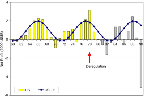
Figure 3-1 shows the best-fit model results as well as industry profits between 1960 and 1990 for comparison. -6 -4 -2 0 2 4 60 62 64 66 68 70 72 74 76 78 80 82 84 86 88 90 Net P rof it (2000 US $B ) US US Fit Deregulation

3.2 U.S. Airline Industry after Deregulation

ATA data of annual profits of the U.S. airlines between 1980 and 2002 were used to analyze the industry after deregulation. The estimated model is provided below and the correlation coefficient is 0.88. Seen from Table 3-2, the estimates of T, t0 and τ are all

significant at 5% level of significance except the estimate of A significant at 10% level.

( )

₍

₎

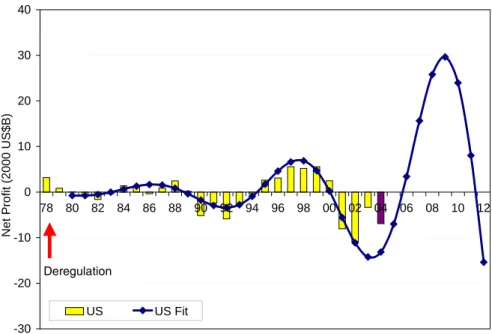
Figure 3-2 shows the best-fit model results as well as industry profits between 1978 and 2003 and the likely result of 2004 for comparison. Because the study was conducted before the end of 2004, the annual profit of 2004 was estimated by prorating the industry profit in the first half of 2004 using Form 41 data [12].

Table 3-2 Regression Results of Net Profit Analysis of the U.S. Airlines after Deregulation

Variable A T t0 τ

Estimate -0.550 11.3 1977.4 7.86

Standard Error 0.287 0.504 0.940 1.43

t statistics -1.92 22.47 2104 5.48

3.2.1 Impact of Deregulation on Profit Cyclicality

Deregulation in 1978 had a profound influence on the U.S. airline industry. Comparison of above two scenarios indicates that deregulation changed the e-folding time significantly. The pre-deregulation model in equation (10) implies an infinite e-folding time, while this parameter becomes finite in equation (11) for post-deregulation condition. As a result, dramatically different behavior was witnessed before and after deregulation. Figure 3-1 illustrates an

oscillation with constant amplitude while Figure 3-2 projects the industry profit to oscillate with increasing amplitude. Moreover, the order of oscillation amplitude in Figure 3-1 and 3-2 is different in order as well. The amplitude of profit oscillation before deregulation in Figure 3-1 is approximately 1 billion dollars, much lower than the amplitude after deregulation in Figure 3-2.

However, comparisons of the two models reveal that the fundamental cycle periods before and after deregulation were almost identical, approximately 11 years. Therefore, it is concluded that although deregulation influenced the oscillation amplitude, it did not change the fundamental profit cycle period of the U.S. airline industry.

-30 -20 -10 0 10 20 30 40 78 80 82 84 86 88 90 92 94 96 98 00 02 04 06 08 10 12 Net P rof it (2000 US $B ) US US Fit Deregulation

Figure 3-2 Net Profit Analysis Results of the U.S. Airlines after Deregulation

3.2.2 Impact of September 11 on Profit Cyclicality

The September 11 event had severely affected the air transportation system in the United States. To evaluate its impact on profit cyclicality, the net profit model was estimated again in equation (12) using the profit data between 1980 and 2000. The correlation coefficient is 0.83 and the regression results are provided in Table 3-3. The estimates of T, t0, and τ are all

significant at 5% level of significance except the estimate of A significant at 10% level. The best-fit model results are shown in Figure 3-3 in comparison with industry profits up to 2003 plus the likely result of 2004.

( )

₍

₎

Table 3-3 Regression Results of Net Profit Analysis of the U.S. Airlines after Deregulation with Data Only before 2001

Variable A T t0 τ Estimate -0.728 12.0 1976.5 9.82 Standard Error 0.398 0.584 0.962 2.80 t statistics -1.83 20.6 2054 3.51 -30 -20 -10 0 10 20 30 40 78 80 82 84 86 88 90 92 94 96 98 00 02 04 06 08 10 12 Net P rof it (2000 US $B ) US US Fit w/o 2001 Deregulation

Figure 3-3 Net Profit Analysis Results of the U.S. Airlines after Deregulation with Data Only before 2001

It is interesting to note that the behavior is not highly dependent on the September 11 event. Comparison of amplitudes in Figure 3-2 and 3-3 indicate that the event exacerbated the profit

oscillation. However, close examination of Table 3-1 through 3-3 shows that the cycle period T of industry profits did not vary significantly.

3.3 World Airline Industry

Following the same methodology, the net profit model of the world airlines was estimated in equation (13). Profit data from ICAO between 1978 and 2002, evaluated in constant 2000 U.S. dollars, were used for analysis. The correlation coefficient is 0.84 and the estimates are significant at 5% level shown in Table 3-4. Figure 3-4 shows the best-fit model results in comparison with the world airlines profits between 1978 and 2003.

( )

₍

₎

Table 3-4 Regression Results of Net Profit Analysis of the World Airlines

Variable A T t0 τ

Estimate -3.00 10.5 1978.9 14.9

Standard Error 1.02 0.328 0.548 4.11

t statistics -2.95 32.1 3612 3.61

3.4 Assumptions and Limitations of Airline Net Profit Model

It is important to note that the net profit model is an extremely simple empirical model that does not address causality or constraints. It is clear that future industry growth will be limited at some point; probably by capital investment as the industry becomes less-appealing to investors due to losses in the down cycle, and/or by capacity and traffic demand as the system reaches the limit of the national aerospace system in the up cycle. Therefore, caution must be taken in applying the models to predict future system behavior and interpreting the projection results.

-25 -20 -15 -10 -5 0 5 10 15 20 25 78 80 82 84 86 88 90 92 94 96 98 00 02 04 06 08 10 12 Net P rof it (2000 US $B )

World World Fit

Figure 3-4 Net Profit Analysis Results of the World Airlines

3.5 Summary of Airline Net Profit Analysis

It was found that the fundamental cycle periods of the U.S. and world airlines were 11.2 and 10.5 years respectively. The net profit analysis of the U.S. airlines indicates that the fundamental cycle period of the industry is endogenous and it has existed in the system even before deregulation. Deregulation did not change the fundamental cycle period of industry profits but had a strong influence on the oscillation amplitude. The September 11 event exacerbated the industry financial status however it did not significantly change the cycle period either. The simple empirical net profit model did not address causality or constraints and is subject to constraints in the future. Nevertheless, the model offers insight on the profit cyclicality of airline industry.

CHAPTER 4

Parametric Model for Capacity

It is known that the presence of phase lag or delay in a control system tends to cause oscillations and make the system less stable. Two potential sources of phase lag were observed through extensive data examination: (1) lag between capacity response and profits, and (2) lag between cost adjustment and profits. This chapter analyzes the relationship between capacity and profits, and discusses a parametric model based on the capacity hypothesis. The cost hypothesis will be discussed in Chapter 6.

4.1 Data Analysis of World Commercial Jet Orders and Deliveries

The relationship between industry profits and world commercial jet orders and deliveries is illustrated in Figures 4-1 through 4-4. Figure 4-1 depicts the world commercial jet airplane orders and deliveries to scheduled passenger and cargo airlines operating worldwide as recorded by ICAO [5]; approximately a two-year time shift can be observed between aircraft orders and deliveries. Figure 4-2 shows the world aircraft orders and net profits, and Figure 4-3 describes the relationship between world aircraft deliveries and net profits [5]. Again, the profit data are recorded by ICAO and they reflect the activity of scheduled passenger and cargo airlines worldwide. An apparent time delay of approximately three years is observed in Figure 4-3 between aircraft delivery peaks and profit peaks.

The annual aircraft delivery data were further regressed with respect to annual profits and traffic (RPK) of several years ago to assess the average delay. The best correlation among these three variables was obtained when average 3-year delay was assumed. As shown below, the

delivery in year t has the best correlation with RPK and Profit three years ago, i.e., RPK and Profit in t-3 year. The equation is in standard econometric form, where the t-statistics of each estimate is presented in the parenthesis immediately below the estimate. The correlation coefficient is 0.90.

Deliveryt = 87 + 0.29 RPKt-3 + 0.027 Profitt-3 (14)

(2.1) (10.9) (5.53)

where RPK is in billions, Profit in billions of dollars and Delivery in aircraft units. All the estimates are significant at 5% level, according to the t-statistics in the parentheses. The regression results are shown in Figure 4-3 for comparison.

0 400 800 1200 1600 2000 1970 1975 1980 1985 1990 1995 2000 2005 A ircraft Units Orders Deliveries

-15 -10 -5 0 5 10 15 1970 1975 1980 1985 1990 1995 2000 2005 A nnual Net P rof it (Current US $ B n ) 0 300 600 900 1200 1500 1800 A ircraf t O rders (unit ) Net Profits Orders

Figure 4-2 World Aircraft Orders and World Airlines Net Profits [5]

-15 -10 -5 0 5 10 15 1970 1975 1980 1985 1990 1995 2000 2005 N e t P ro fi t ( C ur rent U S $ B n ) 200 400 600 800 1000 1200 A irc ra ft D e liv e ri e s ( u n it ) Net Profits Deliveries Delivery Regression

Figure 4-3 World Aircraft Deliveries and World Airlines Net Profits [5]

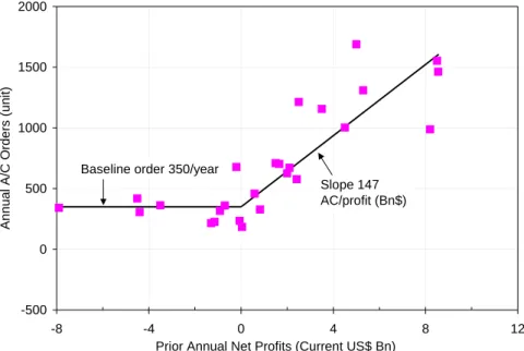
In addition to the delay observation, an asymmetric effect was found to exist between world aircraft orders and net profits. Shown in Figure 4-4, the world annual aircraft orders are plotted against the profits in the prior year. The figure shows that the aircraft orders either grow

with the profits when the industry is profitable or follow a flat trend otherwise. A first-order approximation of this asymmetric effect indicates that the slope of aircraft orders with respect to prior-year profits is on average about 147 aircraft orders per year for each billion dollars of profits, whereas the flat trend is about 350 aircraft orders per year regardless of the magnitude of losses. -500 0 500 1000 1500 2000 -8 -4 0 4 8 12

Prior Annual Net Profits (Current US$ Bn)

Annua

l A/C O

rders (un

it)

Baseline order 350/year

Slope 147 AC/profit (Bn$)

Figure 4-4 Asymmetric Effect between World Aircraft Orders and World Airlines Net Profits

4.2 Capacity Hypothesis

It is known that the presence of phase lag or delay in a control system tends to cause oscillations and make the system less stable. Figure 4-5 presents a generic control system with phase lag that is adopted from Palm’s book [13]. The difference between the input and output is the error that needs to be corrected by the system; however, due to the presence of delay D, the correction will not act on the system (Plant G(s)) and update the output until D time later. Because of delay, the output of such generic system will oscillate around input and the correction item will oscillate around zero.

e-Ds

(Delay)

Input Correction e-Ds _PlantG(s) Output (Delay)

Input Correction _PlantG(s) Output

Figure 4-5 Block Diagram of a Generic Control System with Phase Lag (adopted from Palm’s book [13])

From above data analysis, approximately 3-year delay was observed between aircraft deliveries and industry profits. Applying above generic control model to airline industry and assuming capacity as the output, the capacity hypothesis was that the phase lag in capacity response caused system oscillation.

4.3 Parametric Model for Capacity

A parametric model was developed based on the capacity hypothesis and the block diagram is shown in Figure 4-6. Shown in the figure, the output is the capacity offered by the system that has units of available seat-miles (ASM). The input of the system is the demand, which also has units of available seat-miles in order to match the units of capacity. The difference between the demand and the capacity is capacity shortfall, which again has units of available seat-miles. Airlines order airplanes based on the capacity shortfall and their ordering strategies. The control gain K in the model represents the overall aggressiveness in the ordering process, and has units of ASM ordered per year per unit ASM shortfall. The delay D represents the lag between capacity shortfall and deliveries in the system and has units of years. Assuming airlines’ pricing activity is based on capacity shortfall, capacity shortfall is correlated with profits through constant C, and the delay D also represents the lag between profits and deliveries. Because of

the delay, the new deliveries will not add into the total capacity until D years later. The closed-loop transfer function of the capacity parametric model is

s Ke s Ke s H Ds Ds − − + = 1 ) ( (15) K _(Delay)e-Ds Demand Capacity

Shortfall Order Delivery

s 1 Capacity Capacity C Profit K _(Delay)e-Ds Demand Capacity

Shortfall Order Delivery

s

1 Capacity

Capacity

C Profit

Figure 4-6 Block Diagram of Capacity Parametric Model

4.4 Root Locus Analysis of System Stability

Based on the closed-loop transfer function, a root-locus analysis was performed to analyze the stability of above parametric model and the main branch of root-locus is shown in Figure 4-7.

ω_crit, K_crit Im Re

∞

→

K

K

←

0

Unstable

Unstable

Stable

Stable

∞

→

K

K

←

0

Unstable

Unstable

Stable

Stable

∞

→

K

K

←

0

Unstable

Unstable

Stable

Stable

Figure 4-7 Root Locus of Capacity Parametric Model

The equation for root-locus analysis is

0

1+ − =

s

At the critical point where the root locus crosses over the imaginary axis j

s=ω (17)

Substituting s into equation (16), one obtains

(18) ⎪⎩ ⎪ ⎨ ⎧ = − = 0 ) sin( 0 ) cos( D K D K ω ω ω

Solving for delay D and gain K (K>0)

⎪ ⎪ ⎩ ⎪ ⎪ ⎨ ⎧ = = = + = ω ω ω π π ω ) sin( ... 2 , 1 , 0 2 2 D K n n D (19)

Therefore, at the critical point shown in Figure 4-7, the following relationship holds

⎪ ⎪ ⎪ ⎩ ⎪ ⎪ ⎪ ⎨ ⎧ = = = = = D K D T D T crit crit crit crit crit 2 4 2 2 π ω π π ω (20)

where ωcrit is the critical frequency at which the system oscillates with constant amplitude,

is the oscillation cycle period, and is the critical gain corresponding to

crit T

crit

K ωcrit.

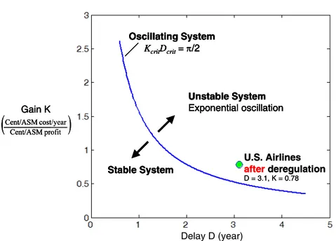
The relationship between the system stability and the values of delay and gain implied by the root-locust analysis is better illustrated in Figure 4-8. The line in the figure indicates the boundary that maintains the system stable. Systems on the boundary will just oscillate with constant amplitude and have the relationship described in equation (20). Shown in Figure 4-7, the system will become unstable when its poles cross over the imaginary axis and enter into the right-hand side of s-plane, i.e., when ω >ωcrit and/or . This corresponds to the area in

Figure 4-8 that is above the stability boundary. Systems in this area will oscillate exponentially.

crit K K>

The area below the stability boundary represents the stable region and corresponds to the left-hand side of s-plane in Figure 4-7.

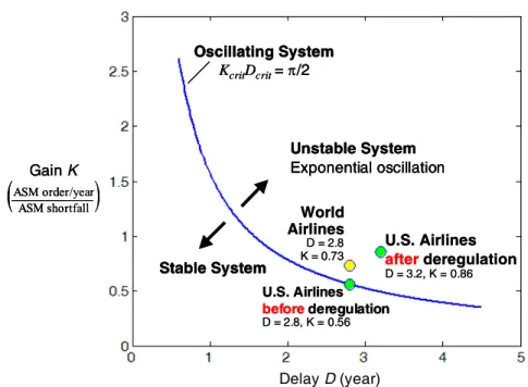
Therefore, the system stability is dependent on the delay and gain values and its location on the map shown in Figure 4-8. To understand the profit stability of airline industry, it is necessary to determine the parameters that represent the U.S. and world airlines and locate them on the map. Oscillating System KcritDcrit= π/2 Unstable System Exponential oscillation Stable System

(

)

(

)

(

)

Figure 4-8 Relationship between System Stability and Delay/Gain Values

4.5 Determining Parameters in the Capacity Parametric Model

4.5.1 Assumptions

In order to use profit data to determine the delay and gain values which would correspond to the observed oscillations, it was necessary to assume some relationship between profit and capacity shortfall. A simple assumption was postulated that the aggregate industry profits are proportional to the capacity shortfall, as shown in Figure 4-6

Such assumption implies that profit has the same characteristic equation as capacity shortfall that is described in equation (16), and consequently has the same oscillation frequency and damping ratio as capacity shortfall. Therefore, it offers a way to determine the delay and gain values using the results of previous airline net profit analysis. Specifically, the fundamental cycle period T and e-folding time τ found in Chapter 3 for the U.S. and world airlines were used to compute the delay and gain values in the following.

4.5.2 Derivation

In general, the complex conjugate poles in the root-locus can be written in the form

j

s=−ξω ±n ωd (22)

Substituting s into equation (16), one obtains

(23) ⎪⎩ ⎪ ⎨ ⎧ = − = + − 0 ) sin( 0 ) cos( D Ke D Ke d D d d D n n n ω ω ω ξω ξω ξω

Under above assumption, ωd andξωn in equation (23) are determined from the e-folding

time τ and the fundamental cycle period T according to the relationship defined in equation (3), that is, ωd =2πT and τ=− 1ξω_n.

Solving for D and K for the main branch,

(

)

(

)

4.5.3 Parameters for the Airline Industry

Using equation (24), the delay and gain values for the U.S. and world airlines were computed from the e-folding time τ and fundamental cycle period T that were estimated in Chapter 3 (Table 3-1, 3-2 and 3-4). The results are summarized in Table 4-1, including the critical gain that is calculated with respect to delay according to equation (20).

Seen from the table, the computed delay for the world airlines is 2.8 years. This is consistent with the observed average 3-year delay between the world airlines profits and aircraft deliveries found in section 4.1. This consistency indicates that capacity could influence profits. The gain for the world airlines is 0.73 annual ASM ordered per ASM shortfall, that is, 73% of capacity shortfall is fulfilled annually. The gain is about 30% larger than the critical value, indicating an unstable system.

Table 4-1 Delay and Gain Estimates of the U.S. and World Airlines under Capacity Hypothesis

T τ D K Kcrit

Airline Industry

Year

(

)

World 10.5 14.9 2.8 0.73 0.56

U.S. before Deregulation 11.2 ∞ 2.8 0.56 0.56

U.S. after Deregulation 11.3 7.86 3.2 0.86 0.49

Similarly, the computed delays for the U.S. airlines before and after deregulation are consistent or close to the observed average 3-year delay for world aircraft deliveries. However, the gain for the U.S. airlines after deregulation is approximate twice of the critical gain, indicating an even-more unstable system. In contrast, the computed gain for the U.S. airlines before deregulation is equal to the critical value, representing a system that oscillates with constant amplitude.

The delay and gain values determined in Table 4-1 are plotted in Figure 4-9 to illustrate the profit stability of the U.S. and world airlines. Seen in the figure, the U.S. airlines before deregulation is located right on the stability boundary, while the U.S. airlines after deregulation and the world airlines all fall in the unstable region. Moreover, the U.S. airline industry after deregulation is positioned further from the stability boundary than the world airlines, indicating it’s more unstable than the latter.

Oscillating System KcritDcrit= π/2 Unstable System Exponential oscillation Stable System World Airlines D = 2.8 K = 0.73 U.S. Airlines after before deregulation D = 3.2, K = 0.86 U.S. Airlines deregulation D = 2.8, K = 0.56

(

)

Gain K Delay D (year) Oscillating System KcritDcrit= π/2 Unstable System Exponential oscillation Stable System World Airlines D = 2.8 K = 0.73 U.S. Airlines deregulation D = 3.2, K = 0.86 U.S. Airlines deregulation D = 2.8, K = 0.56 after before Oscillating System KcritDcrit= π/2 Unstable System Exponential oscillation Stable System Oscillating System KcritDcrit= π/2 Oscillating System KcritDcrit= π/2 Unstable System Exponential oscillation Unstable System Exponential oscillation Stable System Stable System World Airlines D = 2.8 K = 0.73 U.S. Airlines deregulation D = 3.2, K = 0.86 U.S. Airlines deregulation D = 2.8, K = 0.56 World Airlines D = 2.8 K = 0.73 U.S. Airlines deregulation D = 3.2, K = 0.86 U.S. Airlines deregulation D = 2.8, K = 0.56 after before after before

(

)

Gain K

(

)

Gain K

Delay D (year)

Figure 4-9 System Stability and Delay/Gain Values of the U.S. and World Airlines in Capacity Parametric Model

4.6 Factors Contributing to Delay and Gain Values

Some factors in airline operations have been identified to contribute to the delay and gain values in the capacity parametric model. These factors will be further elaborated in Chapter 8 when a more sophisticated model is proposed.

The delay in the airline industry primarily consists of the decision time in placing orders, order processing time and manufacturing lead-time.

Seen in Figure 4-9, the gains representing the world airlines and the U.S. airlines after deregulation are higher than their corresponding critical values for profit stability. Factors contributing to the high gains may include:

• Optimism in total capacity projection that amplifies the capacity shortfall;

• Collective market share perspective is greater than 100%. The collective market share perspective represents the aggregate effect of individual airlines’ projections in market share. For individual airlines, the management usually makes fleet plans based on market share and traffic projections. It is rare for a management to make downward projections of its market share in certain O-D markets and/or across the entire route network of the company. Consequently, the collective market share perspective in each competing O-D market and in total capacity could easily exceed 100%, resulting in significant industry-level over-capacity.

• Aggressiveness when the manufacturers pursue orders. This can happen when a manufacturer offers special deals to particular airlines or markets for the sake of market penetration and/or the market share of the aircraft manufacturer.

• Exogenous factors. Because of the simplicity of the capacity model, the gain has lumped impacts of exogenous factors, such as, the positive impact of high GDP growth on traffic demand and the negative impact of economic recession and war on demand, as well as the influence of fuel price fluctuations on profits.

CHAPTER 5

Simulations of Capacity Parametric Model

The analytical results regarding the delay and gain values determined in Chapter 4 were put into the capacity parametric model for simulation. This chapter summarizes the simulation results with respect to the U.S. and world airlines. The assumption of the dependence of industry profits on capacity shortfall is revisited, and potential approaches to mitigate capacity oscillations are explored.

5.1 Capacity Simulations of the U.S. Airlines

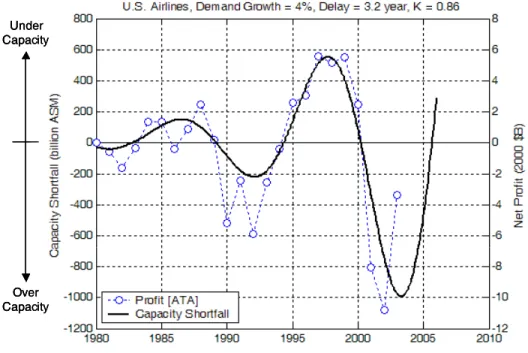
The capacity of the U.S. airlines was simulated by running the capacity parametric model (Figure 4-6) with delay and gain values from the U.S. post-deregulation condition (Table 4-1). The input demand was assumed to grow at 4% per year, based on the average growth rate of the U.S. airlines since deregulation as shown in Figure 1-1. The model was initiated with the industry status in 1980 in terms of profit and associated capacity shortfall, at which time the industry profit was near zero, implying a certain equilibrium achieved between demand and supply.

Figure 5-1 shows the simulation results of demand and capacity in comparison with ATA capacity data. Figure 5-2 shows the results of capacity shortfall plus industry net profits to illustrate the relationship between capacity shortfall and profits. Seen from Figure 5-2, based on the simple capacity model, the industry was approximately 550 billion ASM under-capacity in 1998 while approximately 1000 billion ASM over-capacity in 2003; the capacity shortfall has grown through the cycles. The exponentially oscillating behavior in capacity shortfall is

generally consistent with industry profits. However, the capacity simulation in Figure 5-1 over-predicts the observed variation in capacity data. This indicates that capacity shortfall alone is not sufficient to explain industry profit oscillations.

Figure 5-1 Simulation of Demand and Capacity of the U.S. Airlines

Under Capacity Over Capacity Under Capacity Over Capacity Under Capacity Over Capacity

5.2 Revisiting the Assumption – Cost of Adding Capacity

Aggregate industry profits were assumed dependent on capacity shortfall as (equation (21) in Chapter 4, repeated here for convenience) in order to determine the delay and gain values in the capacity model. If the behavior were solely due to capacity shortfall, constant C in above equation would have the implication of cost or incentive for adding or removing additional capacity. Based on the model results in Figure 5-2, constant C was estimated by regressing the profit data with respect to capacity shortfall via least-square. The value of constant C was found to be approximate 1 cent (2000$) per ASM in capacity shortfall, implying that the cost or incentive for adding or removing one available seat-mile to fulfill the capacity shortfall will lead to approximately one cent (2000$) in profit or loss. Such estimation is preliminary given the simplicity of the model; however, it illustrates the potential interaction between capacity and profit.

Capacity) C(Deamnd

Profit= −

5.3 Capacity Simulations of the World Airlines

The capacity of the world airlines was also simulated by similarly setting the delay and gain in the model to the values for the world airlines provided in Table 4-1. The demand growth rate was set to 4.7%, the average worldwide growth rate (Figure 1-5). The model was initiated with the industry status in 1980 in terms of profit and associated capacity shortfall.

Simulation results of demand and capacity of the world airlines are shown in Figure 5-3 in comparison with ICAO capacity data. The model also simulates the aircraft orders in terms of ASM, as shown in the block diagram (Figure 4-6). In order to compare the results with actual order data, the simulated aircraft orders in ASM were converted to aircraft unit orders by dividing the average aircraft utility. The average aircraft utility of the U.S. airlines, that was 190

million ASM per aircraft per year as discussed in Appendix A, was used in the conversion. The converted order simulations are shown in Figure 5-4, in comparison with the world aircraft order data from ICAO and the baseline order that was 350 aircraft per year as shown in Figure 4-4.

Figure 5-3 Simulation of Demand and Capacity of the World Airlines

Again, the capacity simulation in Figure 5-3 over-predicts the observed variation in capacity data. Seen from Figure 5-4, the simulation of orders is generally consistent with world aircraft orders. There is a positive offset that the model does not represent and it is consistent with the asymmetric effect between profitability and aircraft orders shown in Figure 4-4. This nonlinear asymmetric effect was not included in the capacity model for simplicity reason. Such effect should not be ignored and is included in a more sophisticated model proposed in Chapter 8 in order to better model the dynamics of airline industry.

Therefore, given the simplicity of the model, it is concluded that the capacity model captures some system behavior. The capacity hypothesis appears valid and capacity response appears to be one potential driving factor of the system behavior. However, simulations indicate that capacity shortfall alone is not sufficient to explain the industry dynamics. There is a need to look at other factors such as cost effects, as to be discussed in Chapter 6.

5.4 Mitigating System Oscillations

Assuming the system stability can be modeled by the simple capacity model, the capacity parametric model was used to explore potential ways to mitigate instability. The stability relationship shown in Figure 4-8 suggests that the system could be stabilized by reducing its delay and gain below the stability boundary.

As an illustration, simulations were performed with different delays while holding the gains unchanged. Figure 5-5 depicts the simulation results with respect to the U.S. airlines for different delay values. Given the condition that the gain is held unchanged, the capacity of the U.S. airlines would become stabilized if the delay were reduced from 3.2 years to 1.8 years.

Similarly, the world capacity would stabilize if the delay were reduced from 2.8 year to 2.2 years, shown in Figure 5-6.

Figure 5-5 Mitigating Capacity Oscillations of the U.S. Airlines

5.5 Summary of Capacity Parametric Model

By hypothesizing the lag in capacity response caused system oscillation, the model identified capacity response as one potential driving factor of the system behavior. For this model, the system stability depends on the delay between aircraft orders and deliveries and the aggressiveness in airplane ordering. Assuming industry profits correlated to capacity shortfall, the delay and gain were calculated and the results were consistent with the observed delay between world aircraft deliveries and net profits. Since the gain in the model has lumped impacts of exogenous factors, exaggerated capacity response was observed in simulation. This indicates capacity shortfall alone cannot fully explain the industry dynamics and there is a need to look at other factors such as cost effects. The model also indicates reduced delay may help to mitigate system oscillations.