An analysis of SIFT object recognition with an emphasis on landmark detection

(1)

An Analysis of SIFT Object Recognition with an Emphasis

on Landmark Detection

by

Benjamin Charles Ross

Submitted to the Department of Electrical Engineering and Computer Science

in partial fulfillment of the requirements for the degree of

Master of Engineering

at the

MASSACHUSETTS INSTITUTE OF TECHNOLOGY

September 2004

@

Massachusetts Institute of Technology 2004. All rights reserved.

Author ...

Department of

ectrical Engineering and Computer Science

July 1, 2004

Certified by ...

. . . .

....

. i p y . . .. . . ... .. ... ...

Trevor J. Darrell

Associate Professor

Thesis Supervisor

Accepted by ...

A&ftu'r C. Smith

Chairman, Department Committee on Graduate Students

MASSAOHUSMTS yl145 "

(2)

(3)

An Analysis of SIFT Object Recognition with an Emphasis on Landmark Detection

by

Benjamin Charles Ross

Submitted to the Department of Electrical Engineering and Computer Science on July 1, 2004, in partial fulfillnent of the

requirements for the degree of Master of Engineering

Abstract

In this thesis, I explore the realm of feature-based object recognition applied to landmark detection. I have built a system using SIFT object recognition and Locality-Sensitive Hash-ing to quickly and accurately detect landmarks with accuracies rangHash-ing from 85-95%. I have also compared PCA-SIFT, a newly developed feature descriptor, to SIFT, and have found that SIFT outperforms it on my particular data set. In addition, I have performed a relatively extensive empirical comparison between Locality-Sensitive Hashing and Best-Bin First, two approximate nearest neighbor searches, finding that Locality-Sensitive Hashing in general performs the best.

Thesis Supervisor: Trevor J. Darrell Title: Associate Professor

(4)

(5)

Acknowledgments

To my parents and friends, for always being there for me. To Brian, Naveen, and Ellie, for spending late nights with me while I worked on my thesis. To my thesis advisor, Trevor Darrell, for his endless support and help. To Greg and Kristen for their assistance with

LSH and BBF. To Mike, Louis-Philipe, Kate, Mario, Neal, Ali, and Tom, for dealing

with my numerous questions. To Valerie and Jess for graciously allowing me to use their photos for use in my landmark recognition system. David Lowe for his assistance with the implementation of SIFT. To Yan Ke and Rahul Sukthankar for their assistance with PCA-SIFT.

5

(6)

(7)

5.3.1 Tree Construction ... 5.3.2 Tree Searching ... 5.3.3 The BBF optimization ... 5.4 Locality-Sensitive Hashing . . . . 5.5 Comparison . . . . 5.5.1 Non-Empirical Comparison . . . . 5.5.2 Empirical Comparison . . . . 5.5.3 Discussion . . . .

6 Hypothesis Testing and Integration

6.1 Hypothesis Testing . . . .

6.1.1 Hough Transform . . . . 6.1.2 Least-Squares Affine Transform 6.1.3 Accepting an Hypothesis . . . 6.2 Integration . . . . Verification 7 The Application 7.1 Choice of System 7.2 Data Collection . 7.3 Featureless Models 7.4 Experiments . . . . . . . . . . . . . . . . . . . . 41 42 44 44 45 46 46 49 49 51 51 51 54 55 57 59 60 61 62 67 67 68 68 69 71 73 73 74 75 75

(9)

7.5 D iscussion . . . .

8 Contributions

8.1 Future W ork . . . .

A Data Set

B False Positive Set

C Nearest-Neighbor Test Data Set

77 83 83 85 103 107

(10)

(11)

List of Figures

2-1 An example of an object with a specular highlight . . . . 22

2-2 Affine transformations used to simulate camera rotations . . . . 23

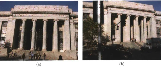
2-3 Features produced by Good Features to Track on two landmark images . . 25

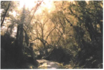
2-4 A view of a forest . . . . 28

2-5 Pyramidal description of an image . . . . 29

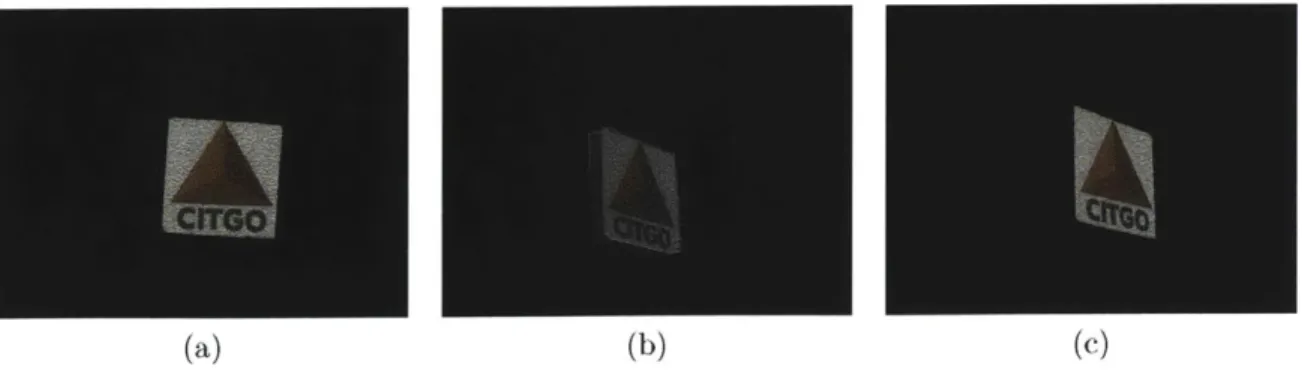
2-6 The Citgo image Gaussian blurred with different variance levels . . . . 31

3-1 Pyramidal gaussian scale space . . . . 35

3-2 Detection of maxima and minima of DOG images . . . . 35

3-3 Selecting keypoints by determining whether the scale-space peak is reasonable 37 3-4 Example images that show why keypoints along edges are undesirable . . . 37

4-1 A view of the SIFT descriptor . . . . 43

4-2 SIFT vs. PCA-SIFT on a relatively difficult data set of 15 models . . . . . 47

4-3 SIFT vs. PCA-SIFT on a relatively difficult data set of 15 models using Mahalanobis-like distances . . . . 48

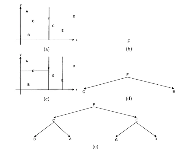
5-1 Kd-Tree Construction . . . . 52

5-2 A Kd-Tree without any internal nodes that reference data points . . . . 53

5-3 Hypersphere intersection in a Kd-T'ee . . . . 53

5-4 An observation about hypersphere-hyperrectangle intersections in Kd-Rees 55 5-5 Kd-Tree performance for gaussian-sampled data in 1, 2, 4, and 20 dimensions 56 5-6 Input of LSH Data . . . . 59

5-7 Error of LSH and BBF as a function of the number of distance calculations 64 5-8 Error of LSH and BBF as a function of computation time in milliseconds 65 5-9 LSH vs. BBF on SIFT features descriptors . . . . 66

(12)

6-1 Two example model views of the Citgo sign ... ...

7-1 Examples of models that could not be reliably detected by the system ... 7-2 Examples of models used in David Lowe's SIFT experiments . . . .

7-3 Data set A with and without LSH, and with and without integration at

optim al settings . . . . 7-4 Data set B with and without LSH, and with and without integration at

optim al settings . . . . 7-5 Average matching times in terms of the time taken to perform a query with integration and without LSH . . . .

A-1 Model 000 A-2 Model 001 A-3 Model 002 A-4 Model 003 A-5 Model 004 A-6 Model 005 A-7 Model 006 A-8 Model 007 A-9 Model 008 A-10 Model 009 A-11 Model 010 A-12 Model 011 A-13 Model 012 A-14 Model 013 A-15 Model 014 A-16 Model 015 A-17 Model 016 A-18 Model 017 A-19 Model 018 A-20 Model 019 A-21 Model 020 A-22 Model 021 71 76 76 78 79 80 . . . . . . . . . . . . . . . . . . . . . . . . . . . . . . . . . . . . . . . . . . .. . . . . . . . . . . . . . . . . . . . . . . . . . . .

(13)

A-23 M odel 022.. . . . .. . . .. . . .. . . . .. . . . . 98 A-24 M odel 023.. . . . ... . .. . . ... . . . . .. . . . .. . 98 A-25 M odel 024.. . . . .. . . .. . ... . . . .. . . . . 99 A-26 Model 025 ... 100 A-27 M odel 026 ... 100 A-28 M odel 027 ... 101 A-29 M odel 028 ... 101 A-30 Model 029 ... 102

(14)

(15)

List of Tables

5.1 The information contained in each Kd-tree node . . . . 52

(16)

(17)

Chapter 1 Introduction

The raw computational power of the computer has increased tremendously over the past few years. For example, the number of transistors in the average processor has consistently doubled every 2 years, resulting in CPU speeds that were unheard of even just a couple years ago. One of the major benefits of this increase in computational power has been a steady rise in the number of computer vision applications. Computer vision problems once thought impossible to solve in any reasonable amount of time have become more and more feasible.

Perhaps one of the most important examples of such problems is efficient, accurate object recognition. That is, given an image of a scene, the computer must return all objects that appear in that scene. Furthermore, if no objects from the scene are "known" to the computer, it must not detect any objects.

There are a wide variety of approaches to this problem. Some of them attempt to extract a global description of the entire image, and utilize this description as a means of matching the particular object. This is a useful approach when a model of the background behind the object is known, so that it can be thus subtracted from the image, making detection less prone to errors.

To illustrate this global approach, take the problem of determining whether a face exists within an image. A global method would determine if the image in its entirety implies that a face exists within it. One night, for example, have a template of a face, and attempt to match that entire template to the image.

Another way to approach the problem is to extract local salient regions, or features, on

(18)

the model image, and determine if enough of these appear on a given query image. More

specifically, something known as a feature extractor is used to extract points on the image

which are likely to be salient across various camera viewpoints. The image is then sampled

around every feature, forming feature descriptors. On the query image, the same operation

is performed, and each feature descriptor extracted from it is matched to the closest feature descriptor on the model images. If enough features are found that they form a consistent representation of an object, a match is declared. This method is known as Feature-Based

Object Recognition.

In our example of determining whether a face exists within an image, the feature based approach would be to extract various salient features on the image, such as a nose, a set of eyes, ears and a mouth. Then, it would match those features to a model of a face, all the while ensuring that the features are in their correct orientations.

One might immediately assert that the local feature-based recognition model is better, because by dividing the image into smaller regions, detection can be made more robust to changes in pose. Furthermore, if there is no available background model, global detection becomes even worse, because the entire background in the image can become incorporated into the global feature for the image.

Yet there are a few advantages to a global model of object recognition, especially if some of the background can be subtracted from the image. Most importantly, the feature-based model relies on there being a large number of extractable features on the object in question. For example, applying feature-based object recognition to the task of recognizing an apple would not be very fruitful, as there are very few salient features on an apple that could be extracted. In such a case, feature-based object recognition often fails, and often a global recognition approach would produce better results.

Nevertheless, this paper is devoted to the study of the feature-based approach to object recognition. In a small application, I have found that it is indeed the fact that objects with very few distinguishable features are difficult to recognize using a feature-based object recognition model. I have built an application that recognizes relatively salient objects quickly with accuracies of 85%. I concentrated on the detection of buildings and landmarks, however, this approach can easily be extended to recognizing other objects. In this particular application, I eventually use SIFT feature extraction and object recognition, developed by David Lowe [13] [11], although my initial recognition applications utilized other methods.

(19)

In the past, there has been a great deal of research in feature-based object recognition, yet the results were very limited in the number of objects it could recognize, and any large image deformation would produce extremely poor results. More often, a global method of object recognition was used, and feature extractors were mostly applied to the problem of tracking. Tracking involves extracting features from an image, then using those features as points to track using optical flow [7] [3]. Only recently, with the work of Schmid and

Mohr [16], and Lowe [13], has feature-based object recognition been able to handle the large

image deformations necessary for accurate and extensible object recognition.

Once it was realized that feature-based object recognition could be applied to large image deformations, there have been a tremendous number of interesting applications. Perhaps the most interesting application is Video Google [18]. Utilizing the same type of metrics used in text-based searching, Video Google attempts to create an efficient image-based search of a video sequence. Thus, a user can search for the occurrence of a particular object within a scene, and obtain results in descending order of their score. Rather than simply performing a brute force search of the object throughout every image sequence (which could take a tremendous amount of time), they employ a method of object localization in each frame by extracting regions based on maximizing intensity gradient isotropy. Thus a set of objects are obtained from each frame a priori, and searching can be done much more efficiently.

My thesis will concentrate on highlighting the four major stages of feature-based object recognition, all the while introducing other methods of approaching each one. These four stages are as follows:

1. Feature Extraction: Salient features are extracted from the image in question.

2. Feature Description: A local sampling around each feature, known as a feature

descriptor, is obtained. It is often then represented in some fashion, for example by

histogramming the values of the pixels in the region.

3. Feature Matching: For each feature in the query image, its descriptor is used to find its nearest-neighbor match among all stored features from all the objects in memory. This is often the most time-intensive step, and thus a faster, approximate nearest-neighbor matching algorithm is often used.

4. Hypothesis Testing: This step determines which of the matches are reasonable, and declares whether portions of the query image represent objects stored in memory. This

(20)

is normally done by finding an approximate affine transformation which transforms each feature on the model image into those on the query image.

The second chapter of this thesis will give a broad overview of both the first and second stages of feature-based object recognition, and will discuss my initial approaches when I first began work on this thesis. In this chapter, I also motivate the need for a scale-space representation of an image. As SIFT is deeply rooted in scale-space theory, this leads us into chapter three, where I introduce SIFT feature extraction, and thus begin again in detail with the first stage listed above. In chapter four, I describe the second stage by introducing the SIFT feature descriptor. In this chapter, I also compare SIFT's descriptor to a recently developed feature descriptor known as PCA-SIFT.

Chapter five then tackles the third stage of object recognition, feature matching, by describing two prominent approaches to approximate nearest neighbor matching, Best Bin

First Trees (BBF), the method taken by David Lowe in his SIFT paper, and Locality-Sensitive Hashing (LSH). In chapter six, I describe hypothesis testing, the fourth and final

stage of feature-based object recognition. I also discuss methods of maintaining a server of objects that can be queried to recognize images supplied by a user. In chapter seven, I show the results of an application that uses the optimal combination of SIFT and the other methods introduced in this thesis to perform landmark detection. Finally, I conclude with chapter eight, which summarizes my thesis and discusses possible future work in the field.

(21)

Chapter 2 Initial Approaches to Feature

Extraction and Descriptors

This chapter discusses my initial approaches to feature-based object recognition, as well as a brief overview of feature extraction methods and feature descriptors in general. It will also motivate the need for a scale-space image representation that will improve the quality of image recognition by detecting features along multiple scales.

2.1 Feature Extraction

The goal of feature extraction is to determine salient points, or features on an image. These

features are used to match against features in other images to perform object recognition (as discussed earlier). For any feature-based object recognition task, we wish that our features have the following properties:

1. Salient: Salient features will be those that are the most invariant to noise and changes in orientation. For example, in choosing features for a building, an ornament on the doorway would perhaps be a better than the doorway itself.

2. Scale-invariant: This means that the same features will be found regardless of how we might have scaled the image. Thus, the distance fr'oim the object to the camera should not cause a change in the features produced.

3. Rotation-invariant: If we rotate the image, we should find the same features. Note that this is different from rotating the camera when observing an object. We simply

(22)

mean here that if the 2-dimensional image of our object is rotated, then we should find the same features.

4. Illumination-invariant: We should find the same features regardless of the lighting conditions. This is a notoriously challenging problem in computer vision. A partic-ularly difficult situation occurs when an object has a specular highlight (see figure 2-11).

5. Affine-invariant: This effectively means that if we perform an affine transforma-tion on the image of the object, the same features will be found. In other words, we can sheer, rotate, scale, and/or translate the image without any loss of the original features. We would like our feature extractor to be affine invariant because any rea-sonably small camera orientation change can be modeled as an affine transformation.

(See Figure 2-2).

Figure 2-1: An example of an object with a specular highlight. Most feature-based object recognition methods will produce features on or around the specular highlight. Thus, if the object or lighting source is moved, the specular highlight moves, and features near or on the specular highlight will not match consistently with the features of the original object.

We will use these properties throughout the paper when discussing feature extraction methods, especially when determining whether SIFT is a reasonable feature extraction method.

My initial experiments used a feature extraction algorithm known as "Good Features to Track", developed by Jianbo Shi and Carlo Tomasi [17]. As the name of the algorithm implies, their approach was to find points on the image that are good for tracking purposes.

(23)

(a) (b)

Figure 2-2: Affine transformations used to simulate camera rotations: in (c), an affine transformation is applied to (a) to appear like (b).

More specifically, their algorithm outputs a set of salient points so that if the camera is moved, many of the same points will be produced. The general application of Good Features to Track is to determine salient features on an initial image, then track those features over time using optical flow. This is of course better than tracking every single point, since not every point at some frame I will be apparent at some later frame J.

2.1.1 Good Features To Track

Good Features To Track (GFT) [17] uses a simple affine model to represent an image J in

terms of an image I:

J(Ax + d) = I(x) .

A good tracking algorithm would have optimal values of A and d, and thus minimize the dissimilarity e taken over a window W surrounding a particular feature:

c JJ [J(Ax + d) - I(x)]2dx

We wish to minimize this residual, and thus we differentiate with respect to d and set it equal to zero. Using the Taylor expansion J(Ax + d) = J(x) + gT(u), and [17], this yields the simple 2 x 2 system

Zd = e, where

(24)

z 2

9X 9Xgy

and

e =,/J

[I(x) - J(x)]

K I

dx

J Jw gy

It turns out that if the eigenvalues of A, and A2 of Z are sufficiently large, and also if A,

is sufficiently larger than A2, then the feature at x is a "good feature to track." The first

condition very often implies the second, and thus, it is only required that

min(Al, A2) > A,

where A is a predefined threshold.

2.1.2 Discussion

I found that GFT performed relatively poorly when applied to the task of feature-based object recognition. This is mainly due to its assumption that the deformations between

adjacent frames are small [17]. In object recognition, it is often required that features

be matched across relatively large image deformations. Thus, when the change in camera orientation was large, very few features maintained their original locations on the object

(see figure 2-3).

Although it is possible to extend the formulation of GFT to model the feature window deformations, thereby allowing larger image deformations, [17] states that doing so would lead to further errors in the displacement parameters of each feature. Thus, using GFT for use in feature-based object recognition cannot possibly produce reasonable results.

Regardless, I continued to experiment with Good Features to Track, not to produce an application with any reasonable results, but simply to explore the realm of feature-based object recognition. This led me to experiment with feature descriptors, which are aptly

named local descriptions of the image surrounding each feature.

(25)

(a) (b)

Figure 2-3: As expected, Good Features to Track produced relatively poor features for object recognition. These features were produced with a A threshold of 0.001, and it was enforced that each feature be at least within 10 pixels of each other.

2.2 Feature Descriptors

Once we have a list of features, we must appropriately sample the image around it. This

sampling of pixels, when represented in some fashion, is known as a feature descriptor,

because it describes the local image properties of that feature.

My initial feature descriptor was a 2-dimensional Hue-Saturation (H-S) color histogram of the circular patches surrounding each feature. Matching was done by correlation of each histogram. The descriptor was also normalized for illumination invariance. This worked reasonably well, as the histogram model was relatively robust to noise. Furthermore, it has been shown that the hue and saturation values of an image are relatively invariant to illumination changes, albeit only to pure white light.

However, when more than a few objects were added to the database, the object matching began to fail miserably, and performance degraded to less than 10%. This makes sense, since although the H-S model is relatively robust to noise, it also allows for a great degree of false positives. This is due to the fact that a histogram of color values, by nature, under-describes an image patch. That is, if we simply rearrange the order of pixels in the image patch, the same histogram will be produced.

For this reason, I attempted to make the descriptor more specific by incorporating Hu Moments into the description of the local patch.

(26)

2.2.1 Hu Moments

Hu Moments [8] are a set of seven orthogonal moment invariants that are proven to be rotational-invariant, scale-invariant, and reflection-invariant. They have been used in the past in simple character recognition [20] and other simple feature-based recognition prob-lems.

The set of 7 moments can be computed from the normalized centralized moment up to

order three, and are shown below as I1 through 17:

II = 7120 + 7102 12 = (7720 - 7702) + 411 13 = (7730 - 3rI12)2 + (37121 - 703)2 14 = (7130 + 7112)2 + (7721 + 7103)2 15 (730- 37r12)(7q30 + 712)[(T/30 + 7112)2 - 3(121 + 703)2] + (3721 - 7703)(7/21 + 7r03)[3(7130 + 712)2 - (21 + 703)2] 16 (n120 - 7702) [(7130 + 712)2 - (7721 + 703)2 + 47111(7130 + 7/12)(rq21 + 7103)]

The 7th moment's sign is changed by reflection, and thus is not reflection invariant per

se. Thus, for my use, this was the most important moment, since it is not reasonable to

(27)

17 = (3?721 - ?703) (730 + ?712) [(q30 + 7712)2 - 3(7721 + 7703)2 + (q30 - 37712)(7712 + 7703)[3(7730 + 7712)2 - (21 + 7703)2]

These moments were combined with the H-S histogram to provide a relatively robust feature descriptor. Matching between descriptors was done by taking a weighted sum of the differences of each Hu moment, summed with a weighted correlation measure of the H-S histograms of the features in question. The optimal weights to use were determined experimentally.

2.2.2 Discussion

Unfortunately, this still proved to be inadequate. There are numerous issues with my approach. As mentioned earlier, using Good Features to Track to produce any reasonable object-recognition application is not very realistic. In addition, it has been shown that both Hu Moments and color histograms do not perform well compared to a host of other prevalent feature descriptors [14].

Eventually, this lead me to discover the paper SIFT [13] [11], which had claimed to produce significantly better results with feature-based object recognition. I introduce SIFT in chapter 3, but before discussing it, it would be worthwhile to discuss something known

as Scale-Space Theory, as SIFT's implementation is deeply rooted in it.

2.3 Scale Space

Suppose we are at the edge of a forest, looking directly at it. (See Figure 2-42) Initially, we might simply view this scene as a 2-dimensional wall, taking in the entire forest at once. We look closer, and begin to see individual trees. If we come closer, we see each individual leaf on the tree. At even closer inspection, we are able to see each vein on a leaf.

Each of these inspections occur at different scales. In viewing a scene, no one scale is more important than the other, and thus analysis of a scene should take all scales into account. In this light, we come to the notion of a scale-space representation of an image.

(28)

Figure 2-4: A view of a forest that shows how scale space can be a useful parameter to add to a description of an image.

We add an additional parameter to our notion of an image, namely scale.

Thus, an image I(x, y) will now include a scale value, and hence become L(x, y, s). In our space representation, L(x, y, 0) := I(x, y). That is, at the finest scale, the scale-space representation will simply be the original image. Then, as the scale value is increased, details should disappear monotonically [10].

2.3.1 Gaussian Scale Space

What is the best way to formalize this concept of scale-space? What operation applied to the image will take us from a scale value of 0 to some arbitrary higher value? The answer came in 1984, when Koenderink described that, under a variety of assumptions, the scale-space representation of a two-dimensional signal must satisfy the diffusion equation:

11

OtL

=

-V 2

L = -(iOx + ayy)L [10].

2 2

where L(x, y, s) is the scale-space representation of the two-dimensional signal I(x, y). The solution of the diffusion equation at an infinite domain is given by a convolution with the Gaussian kernel G.

1 (2 +2)

1 -(x+y)

G(x, y;t)= -e 2f .

(29)

This implies that the most ideal scale-space operator is simply the Gaussian kernel. If we take an original image I and convolve it with a Gaussian kernel, i.e., blur it, the resulting image will be the image's description at a higher scale space level.

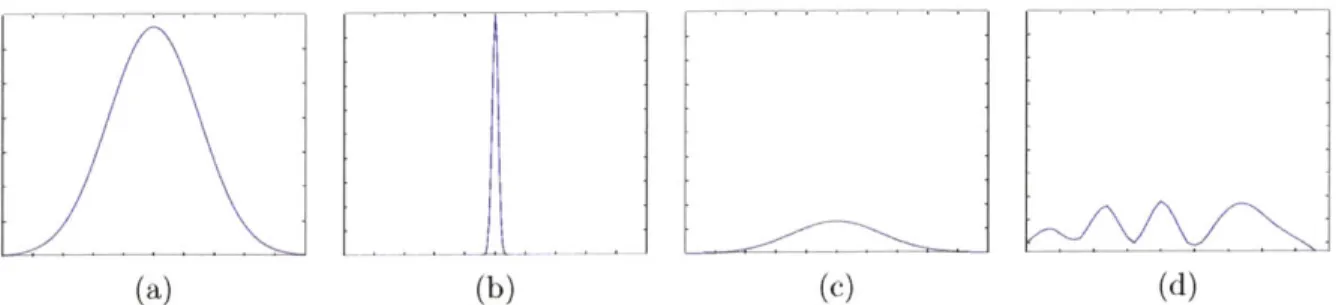
Intuitively, this makes sense: by blurring an image, we suppress fine-scale details on the image. If we blur it again, more details are suppressed. These operations represent the image's traversal through scale-space. Furthermore, we can simply let the imaginary "scale" value be the same as the covariance of the gaussian kernel used to blur the image. Refer to figure 2-6.

2.3.2 Pyramidal Gaussian Scale-Space

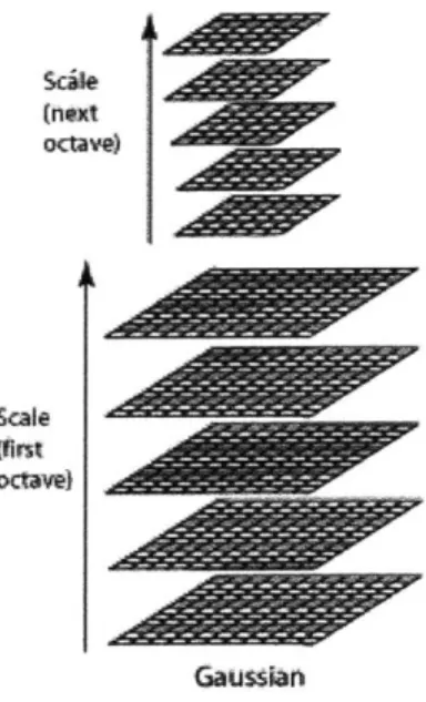
It has been shown beneficial not only to convolve the image with a Gaussian kernel, but also to halve the size of the image every k number of Gaussian blurs. This builds what is commonly known as a pyramidal description of the image.

The pyramid is defined as follows: at the ith level, or octave, of the pyramid, we use the original image scaled by a factor of 2-i. Within each octave, the image is blurred k times, in the same manner as described in subsection 2.3.1. See figure 2-5.

Scale

(Aint octave)

Gausia

Figure 2-5: A 2-octave pyramidal description of an image, with 4 gaussian blurs per octave.

We wish for the effective "scale" to double each octave, and therefore, r, the ratio between the scale-value of each image is given by:

(30)

2 = rk

which, solving for r, becomes

r = 21/k

We let the scale value of the initial image be uo, the initial covariance used to blur the first image in each octave. (This initial blurring may or may not be performed, depending on implementation). Then, the next scale values will be 21/kao, 22/koo, ... , 2(k-1)/koO. In

terms of r, this becomes uor, aor ,., oork- . Then, for the next octave, the first scale

value is 2ao, followed by 2 .21/koo, and so forth.

Note that the scale value is now no longer the same as the covariance level of the gaussian kernel used. It is only this way for the the first octave. For all subsequent octaves, the scale value doubles, while the covariance level starts at ao at each octave and increases by a factor of r until it reaches 2(k-1)/kOO.

2.3.3 Applying Scale-Space to Feature Recognition

When we have a scale-space model of an image, features are no longer detected at the 2-dimensional coordinate (x, y) but at the 3-2-dimensional coordinate (x, y, s). When matching is performed between features on a query image and a model image, we thus match across all scales of a particular image. In this way, matching an image of a model from a great distance becomes easier, as we have already modeled that particular scale of the model in the scale-space representation of the image. Thus, by employing a scale-space representation, we make an attempt at ensuring the scale-invariant property of good feature-extractors mentioned earlier. The features for a particular image are not purely scale invariant, but rather a small subset of the features will likely contain the description of the image at the scale of the query image.

(31)

(a)

(b) (c)

(d) (e)

0 ku

(f) (g)

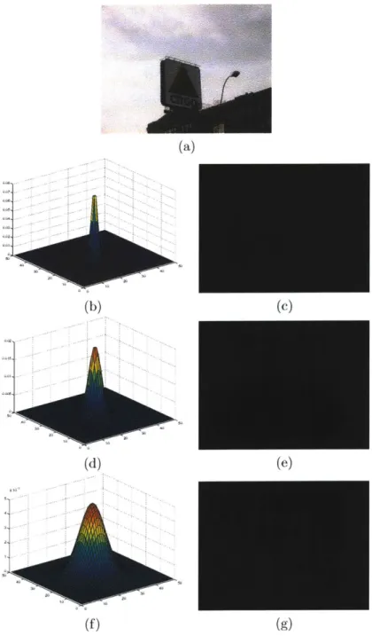
Figure 2-6: The citgo image blurred with Gaussian kernels of different variances. (a) shows the original citgo image. (b) shows an image of the first gaussian kernel, with variance v'2. (c) is the result of blurring the citgo image Gaussian kernel with variance

v'2.

(d)-(g) follow similarly with variance levels 2v'2 and 4V.

(32)

-2.4

Summary and Motivation for SIFT

In this chapter I have discussed my initial approaches to feature-based object recognition, and explored various different feature descriptors. I have also described how a scale-space representation to an image can help to identify features at various scales so that feature extraction can become more scale-invariant. In the following chapter, I introduce and give an overview to SIFT, developed by David Lowe, which utilizes a scale-space representation to perform better feature extraction. Then, in chapter 4, I describe SIFT's feature descriptor, which has shown to perform better than Hu Moments and other methods which I had attempted earlier [14].

(33)

Chapter 3 SIFT Feature Extraction

As motivated in chapter 2, SIFT utilizes a scale-space representation of the image to extract features that are more invariant to scale transformations by finding features on an image at multiple scales. More formally, given an image I(x, y, s), it finds all points (xi, yi, si) such that there is a salient feature on the image at location (xi, yi) and scale si.

There are, generally speaking, four stages in the SIFT algorithm:

1. Scale-space peak selection: The first stage of computation searches over all scales and image locations to identify interest points that are invariant to scale and orienta-tion. It can be implemented efficiently by using a difference-of-gaussian funcorienta-tion.

2. Keypoint localization: At each candidate location, a detailed model is fit to deter-mine location, scale, and contrast. Keypoints are selected based on their stability.

3. Orientation assignment: One or more orientations are assigned to each keypoint based on local image properties.

4. Keypoint Descriptor: The local image gradients are measured at the scale in the region around each keypoint, and transformed into a representation that allows for local shape distortion and change in illumination. [13]

I discuss the first three stages in this section, saving the last for chapter 4, where I discuss both SIFT's descriptor and the newer PCA-SIFT descriptor.

(34)

3.1 Scale-space peak selection

As motivated in Chapter 2, we would like to provide a scale-space representation to the image so that we can select features across multiple scales. This will provide a much greater deal of scale-invariance when performing object recognition.

To review, we wish to describe an image I as

L(x, y, s) = G(x, y, a) * I(x, y)

where G(x, y, a) is the 2-dimensional Gaussian distribution function:

1 -x 2+y2

G(x,y,a)= 2 2

SIFT discretizes space into a series of s values using a pyramidal gaussian scale-space model, as described in chapter 2. That is, it computes a series of sequentially blurred images. There are k blurred images in a particular octave and n octaves. There are thus

nk images in total, representing n different scales and k different blurrings of the original

image.

3.1.1 Difference of Gaussians

SIFT uses these images to produce a set of difference-of-gaussian (DOG) images. That is, at each octave, if there are k blurred images, then there will be k - 1 difference-of-gaussian images. Each image is simply subtracted from the previous. (Refer to figure 3-1). The keypoints detected by SIFT are the extrema in scale-space within each octave of these

k - 1 difference-of-gaussians. Within a particular octave, a difference-of-gaussian function,

D(x, y, a) is computed a.s follows:

D(x, y, a) = (G(x, y, ra) - G(x, y, a)) * I(x, y)

= L(x, y, ra) - L(x, y, 0)

(35)

octavel. Also, r is the ratio between scales given in chapter 2, namely r = 2 /.

(rod

GQcta

Gvs.n(OG

Figure 3-1: A view of how the difference-of-gaussian function is computed. At each scale,

k images are computed, and from that k - 1 difference-of-gaussians are computed [13].

Figure 3-2: Detection of maxima and minima of DOG images is performed by comparing a pixel with its 26 neighbors.

The primary reason for choosing such a function is that it approximates the

scale-normalized Laplacian of Gaussian (oa2V2G). It has been shown that the maxima and

The notation here is a bit sloppy for the purposes of comprehension. When we say L(x, y, a), we mean to say L(x, y, 2 a) where i is the current octave, because s, the scale value, is given by s = 2'a. Furthermore,

I(x, y) is the scaled version of the image for the particular octave i, and thus a better way to notate it would

(36)

minima of this particular function produce better, more stable image features than a host of other functions, such as the Hessian, gradient, and the Harris corner function [13].

We once again can use the diffusion equation to determine understand how a difference of gaussian function approximates the scale-normalized Laplacian of a Gaussian. We take

the heat diffusion equation, (this time parameterized in terms of a instead of t = a2):

49G

=

aV 2

_G

Using the finite difference approximation to a derivative and the previous equation, we have: ,V2G _G G(x, y, ro) - G(x, y, a) 02G =ra -and therefore, G(x, y, ra) - G(x, y, a) ~ (r - 1)o 2 v 2 G .

For a more detailed analysis, refer to [13].

3.1.2 Peak Detection

SIFT determines scale-space peaks functions over 3 difference-of-gaussian images. This is done by a simple comparison with each of its 26 neighbors (9 in the image at a higher scale, 9 in the image at a lower scale, and 8 surrounding pixels at the current scale). Refer to figure 3-2 for a view of how this is done. (For a more detailed explanation, refer to [13]).

3.2 Keypoint Localization

At this point, each scale-space peak is checked to determine if it is a reasonable candidate for a keypoint. This check is important because some peaks might not have good contrast, and other peaks might not be consistent over the 26 sampled pixels. A reasonable peak is determined by modeling it as a 3-dimensional quadratic function, and is described in detail in [13]. Refer to figure 3-3 for examples of reasonable and unreasonable peaks.

(37)

(b)

Figure 3-3: Selecting keypoints by determining whether the scale-space peak (a) shows an example of a reasonable peak in scale space, whereas (b), (c), examples of unreasonable peaks.

is reasonable. and (d) show

it

(a) (b)

Figure 3-4: Example images that show why keypoints along edges are undesirable. (a) shows an undesirable keypoint located along an edge. Any noise could cause the keypoint to traverse the edge along the drawn arrows. (b), on the other hand, shows a much more reasonable keypoint, as it is stable in both directions.

3.2.1 Eliminating Edge Responses

It is also essential that a keypoint does not lie on an edge in the image. At an edge, the peak is well-defined in one direction, but not in the perpendicular direction. Thus, any noise in the image will potentially cause the keypoint to traverse the edge, resulting in poor matching (see figure 3-4). It is possible to determine which peaks are edges by computing the Hessian matrix at the location and scale of the keypoint. This is discussed in detail in

[13].

(38)

3.3 Orientation Assignment

In addition to a position and a scale, each keypoint also has a orientation associated with it. This orientation is determined prior to creating the descriptor, and is done by creating a 36-bin orientation histogram covering a gaussian weighted circular region around each keypoint. The most dominant orientation is determined by finding the bin with the most points. Furthermore, if there exists bins within 80% of the largest bin, another keypoint is created at the same location with that particular orientation. Thus, it is possible for there to be multiple keypoints at the same position in the image, but with different orientations.

3.4 Evaluating SIFT

In chapter 2, we defined a list of desirable properties of good feature extractors. We return to these properties now to observe how SIFT achieves or does not achieve them.

1. Salient: It has been shown that SIFT features are indeed salient, as they approximate the peaks and troughs of the scale-normalized Laplacian of a Gradient of the image. This function has shown to produce the most stable, salient features compared to a host of other feature extraction methods.

2. Scale-invariant: SIFT features are not scale-invariant per se, but the scale-space representation of the image ensures that matching across various scales can be done more accurately.

3. Rotation-invariant: SIFT features are indeed rotation invariant. It is possible that some features will be lost due to the choice of sampling frequency, but at least the majority of features will remain in a consistent position as the image is rotated.

4. Illumination-invariant: The SIFT feature extractor runs on a set of gray-scale images. This in general reduces the positional movement of features when illumination is varied.

5. Affine-invariant: SIFT features are not affine invariant, yet the SIFT descriptor compensates for this by allowing for small changes in the position of the keypoint without a significant change in the descriptor. (refer to chapter 4).

(39)

3.5 Summary

Thus, we now have a list of keypoints selected at peaks in pyramidal scale-space using a difference-of-gaussian image representation. Each keypoint is defined by its position in the image, the scale value at which it was detected, and its canonical orientation. Some keypoints were rejected due to poor stability, and others were rejected if they lied along an edge. Furthermore, some keypoints have the same position in the image, yet different orientation, due to the fact that there might be more than one dominant orientation within a particular feature window. Once we have these keypoints, the next step is to perform a sampling around each to determine its local descriptor. This is the topic of the next chapter.

(40)

(41)

Chapter 4 SIFT Feature Descriptors

Once we have a list of features, we must appropriately sample the image around it. This sampling of pixels, when represented in some fashion, is known as a feature descriptor, because it describes the local image properties of that feature.

Although we have discussed a number of plausible feature descriptors in chapter 2, experiments (see [14]) have shown that the SIFT descriptor performs better than those presented in chapter 2, as well as a host of other feature descriptors, such as template correlation and steerable filters [4].

Thus, I chose to use the SIFT descriptor. However, I have also implemented a descriptor similar to SIFT, known as the PCA-SIFT descriptor (see [9]), since it claims to perform even better than SIFT's descriptor.

This chapter is devoted to discussion of both the SIFT and PCA-SIFT descriptor rep-resentations. The first section will discuss the SIFT descriptor, the second will discuss the PCA-SIFT descriptor, and the third will offer a comparison between the two.

Let us recall where we were once we finished chapter 3's description of SIFT: we have a list of keypoints, each found at a particular scale, orientation, and coordinate location. We now wish to obtain a descriptor representation for each keypoint.

We might consider simply sampling the region at the image corresponding to the fea-ture's scale, and use it as a template for later matching by means of correlation. However, this will cause serious issues. Consider the situation when the template window is rotated by a few degrees, at which point the correlation metric will fail.

(42)

in chapter 3. This entails literally rotating the patch before sampling it into a descriptor vector.

We still have more issues to deal with: What if the location of the keypoint is slightly off? That is, consider a single pixel shift in the feature descriptor. It would then not match the original descriptor.

What is the solution to this problem? David Lowe proposed that instead of sampling actual pixel values, we sample the x and y gradients around the feature location[13] [11]. This method was inspired by a use of the gradient in biological image representations [2]. When gradient information is used, rather large positional shifts are allowed without a significant drop in matching accuracy.

Both PCA-SIFT and SIFT utilize this gradient sampling as a means of forming their feature descriptors. More specifically, both PCA-SIFT and SIFT share the following in common:

1. They sample a square region around the feature in the original gray-scale image. A square sampling region is used rather than the more conventional circular region for ease of implementation and performance gains.

2. They rotate the original sampling using the direction of the most significant gradient direction within the pixels sampled.

3. If the square patch size is of width w, they sample (w - 2) x (w - 2) x gradients, and the same number of y gradients. This gives a set of 2 x (w - 2) x (w - 2) values. In my implementation, the patch size was 41, and thus I had 2 x 39 x 39 = 3042 x and y gradients.

At this point, SIFT and PCA-SIFT differ in their respective implementations, and thus I describe each in turn.

4.1 The SIFT Descriptor

SIFT takes the x and y gradients and computes the resulting set of magnitudes and orienta-tions. Thus, we turn a 3042-dimensional vector of x and y gradients into a 3042-dimensional vector of magnitude and orientations. More specifically, each set of x and y gradients (Xx,y

(43)

t

m"ge grsiients Keypo"w dwcr**x

Figure 4-1: The left figure shows an image patch surrounding a given feature. At each sample point, the orientation and magnitude is determined, then weighted by a Gaussian window, as indicated by the overlayed circle. Each sample is accumulated into "orientation

histogTams". This is simply a histogram taken over all orientations within a particular

region. The length of each arrow corresponds to the sum of the magnitudes of each sample in a particular orientation bin. This figure shows the sampling occurring over 2 x 2 regions, but in the implementation of SIFT, a 4 x 4 sampling is used. The number of orientation bins is 8. Thus, the total size of the descriptor is 4 x 4 x 8 = 128 [13].

and Y,y) is used to compute the magnitude m 'y, and orientation, O

y

by means of the

following equation:

Oxy=tan- l(YX Y xx'y

Thus, we are left with a 3042-dimensional vector containing magnitudes and orientations of pixels surrounding each feature. SIFT reduces this into a significantly smaller vector by

dividing the sampled region into a k x k region (see figure 4-1), and computing a histogram

of gradient orientations within each. By histogrammining the region in this way, the resulting descriptor is made more robust to image deformations.

Prior to placing each gradient in its appropriate histogram, a Gaussian weighting func-tion with a equal to one-half the width of the descriptor window is applied. The purpose of this is to avoid sudden changes in the descriptor with small changes in the position of the window. This is because the gaussian window function gives less weight to gradients near the edge of the window, and these are exactly the gradients that will be affected the most by changes in camera orientation.

(44)

To reduce the possibility of boundary effects, each gradient is placed into the 8 sur-rounding bins as well, each one weighted by its distance to that bin. That is, bilinear interpolation is used to determine the weight of each entry into the histogram.

In chapter 2, we mentioned that specular highlights can cause difficulties with object matching. Specifically, if there is a specular flare near a feature in a query image, and no specular flare in the template image, then that particular feature would not be matched. To attempt to compensate for this, Lowe notices that a specular highlights result in abnormally large gradient values. To compensate, once we have created our full feature vector, gradient magnitudes are cut off at an empirically determined value. Effectively, this "erases" the specular highlight from the feature descriptor. Of course, this cutoff will impact matching negatively in some cases, for example, if an object contains a feature that appears very much like a specular highlight. However, the implementation banks on the fact that this does not happen very often.

4.2 The PCA-SIFT Descriptor

Before we discuss how the PCA-SIFT descriptor works, let us take a moment to understand PCA, since PCA-SIFT is effectively PCA performed on each 3042-dimensional vector of x and y gradients.

4.2.1 Principal Component Analysis (PCA)

Principal Component Analysis, or PCA, is a method of reducing the dimensionality of a

data set by projecting it onto a smaller coordinate space that maximizes the variance along each axis. Using the derivation outlined in [3], the coordinate axes of this coordinate space are simply the eigenvectors of the covariance matrix of the data. That is, if we construct

a NxM matrix A where each N-dimensional mean-free data point is a row in the matrix,

and there are M data points, then we need to find the eigenvectors of the covariance matrix C:

1

C= AAT

M

(45)

C=VEVT

For PCA, recall that we wish to find the vector space such that the variance is maximized in each dimension. Conveniently, Ei,i corresponds to the variance when the data is projected onto the eigenvector located at the ith column of V. Thus, if we desire a k-dimensional coordinate space, we simply need to find those eigenvectors whose corresponding eigenvalues are the k-largest. Then, we obtain the k-dimensional description of the data set by taking the original mean-free data matrix A and projecting it onto the eigenspace given by the those k eigenvectors.

4.2.2 Singular Value Decomposition

It is often the case that computing the covariance matrix C is too costly. Luckily, it turns out that we can simply compute the Singular Value Decomposition (SVD) of the original mean-free data matrix A. From [19], the Singular Value Decomposition of any matrix A returns an orthonormal matrix U, a diagonal matrix S, and an orthonormal matrix V in the following form:

A

= USVT

The proof for why the SVD of the matrix A will produce the eigenvectors of its covariance matrix goes as follows:

C = AAAT

= USVT(USVT)T (using the SVD decomposition A = USVT)

= USVTVSTUT

= USSTUT (because V is orthonormal)

=

AUS2UT

(because S is a diagonal matrix)

= UKUT

Thus, taking the SVD of A will produce the eigenvalue decomposition of C with a

(46)

eigenvectors, and the diagonal elements of _S 2 are the eigenvalues.

4.2.3 PCA Applied to SIFT

The PCA-SIFT descriptor is simply the application of PCA to the original 3042-dimensional vector of x and y gradients [9]. After the 3042-dimensional vectors for each keypoint for a set of training images are obtained, its eigenspace is computed. Then all keypoints extracted from further query images are projected onto this eigenspace. For a more complete discussion, refer to [9].

As the motivation behind PCA-SIFT is to create a descriptor that is both smaller and more accurate than the original SIFT descriptor, the value for the number of dimensions

k should be less than or equal to 128, the original number of dimensions used in the SIFT

descriptor.

4.3 Comparison

PCA-SIFT and SIFT were compared using an implementation of SIFT and my own im-plementation of PCA-SIFT. Tests were run on a data set of 15 models, each consisting of one training image with the background subtracted, and 5 test images. In addition, 30 images were used for determining PCA-SIFT's resilience to false positives (These 30 im-ages were selected randomly from the false positive data set shown in appendix B). The hypothesis-checking model was used as described in chapter 6 of this thesis and [13], and naive (brute-force) nearest-neighbor matching was used. See appendix A for more details

about the data set used.

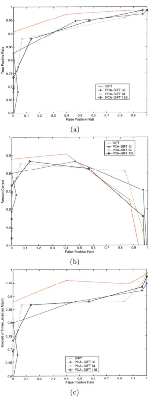
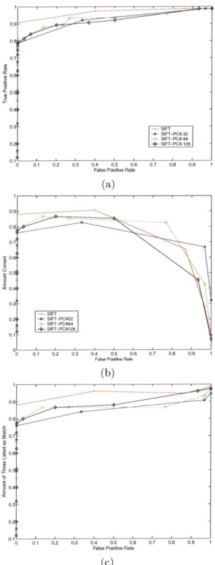
Figure 4-2 shows a comparison of SIFT and PCA-SIFT. Unlike in [9], PCA-SIFT did not perform as well as SIFT. Figure 4-3 shows SIFT vs. PCA-SIFT when a Mahalanobis-like distance metric was used to attempt to improve the performance of PCA-SIFT. This improved the matching accuracy slightly, but still could not rival the SIFT descriptor for this particular data set.

Thus the only possible conclusion, assuming that the results of the PCA-SIFT paper were correct, is that SIFT only performed better on this particular data set. For example, it is possible that PCA-SIFT would perform better on more uniform objects, because it would result in a sparser data set for the gradient descriptors.

(47)

OM9 - 0.9- 0.85-0.8 0.75 0.7,- SIFT -.- PCA-SIFT 32 PCA-SIFT 64 0.65 -4- PCA-StFT 128 0 0.1 0.2 0.3 0.4 0.5 0.6 0.7 0.8 0.9

False Positive Rate

(a) 0.9 0.8 0.7 0.6 0.95 0.8 0.75 0.7 0.65 0.1 0.2 0.3 - SIFT -- PCA-SIFT 32 PCA-SIFT 64 -4- PCA-SIFT 128 0.4 0.5 0.6

False Positive Rate

(b) SIFT -.- PCA-SIFT 32 PCA-SIFT 64 -0- PCA-SIFT 128 0- 0:1 02 0.3 0.4 0.5 0.6 0.7 False Positive Rate

(c)

0.008 0.4

0.8 0.9 1

Figure 4-2: SIFT vs. PCA-SIFT on a relatively difficult data set of a comparison of the receiver-operating curve, (b) shows the amoint the amount of times the correct match was returned.

15 models. (a) shows correct and (c) shows 0.7 0.8 0.9 1

(48)

0.0 0. 0. 0.; 0.; 0. 0.i 0. 0. 0. 0. 0. 0.4 0. 0.1 - SIFT -+ SIFT-PCA32 - SIFT-PCA64 -0-- SIFT-PCA 128 -1 0.1 0.2 0.3 0.4 0.5 0.6 0.7 0.8 0.9 1

False Positive Rate

(a)

0,

0 0.1 0.2 0.3 0.4 0.5 0.6 0.7 0.8 0.9 1

False Posive Rate

(b)

0.1 0.2 0,3 0.4 0.5 0.6 0.1 0.2 0.3 0.4 0.5 0.6 False Positive Rate

(c)

0.7 0.8 0.9 1

Figure 4-3: SIFT vs. PCA-SIFT on a relatively difficult data set of 15 models using a Mahalanobis-like distance function. (a) shows a comparison of the receiver-operating curve, (b) shows the amount correct and (c) shows the amount of times the correct match was returned. - SIFT --- SIFT-PCA32 SIFT-PCA64 -0-- SIFT-PCA128 0.9 0.8, $ 0.7 $ 0.6 0.5 S0.44 0.6 0. 0.1

₀

k'M N ja&! R i? I ! - -- - - - -- --- - ._ I ₀ 7 E 5 4 a 2 9 7 6

(49)

Chapter 5 Descriptor Matching

In any feature-based object recognition system, the performance bottleneck will likely be the matching phase. We wish to find the closest match for some 750 feature points, each consisting of a d-dimensional descriptor, to a set of maybe 50, 000 different features. In such a situation, a brute-force approach is simply not feasible. So, we devote this chapter to the discussion of approximate nearest neighbor solutions. These algorithms sacrifice some of the guaranteed precision of the brute-force approach for greater improvements in speed. We therefore wish to find the algorithm which will return the most accurate matches in the fastest time. I will concentrate on two nearest neighbor algorithms in this chapter: Best

Bin First (BBF), and Locality Sensitive Hashing (LSH).

This chapter will first give a background of nearest neighbor searching, then move on to introduce the naive brute-force approach to nearest-neighbor matching. I will then discuss BBF and LSH in turn, and in the final section, provide an extensive empirical comparison between the two algorithms.

5.1 Background

Let us quickly take a brief overview of the two nearest-neighbor methods that will be discussed in this chapter:

1. Best Bin First, otherwise known as BBF, is the popular approximate nearest neighbor

matching algorithm used by David Lowe in his SIFT paper [13] [1]. It creates a tree-based representation of the data so that only O(log n) scalar comparisons are needed to get to a region where the point "likely" exists. At this point, depending on the

(50)

degree of precision the user desires, further brute force nearest-neighbor searching is done in points surrounding that region.

2. Locality-Sensitive Hashing, otherwise known as LSH, is a hashing-based approach to approximate nearest neighbor matching. Its approach is exactly described in its title: use "locality-sensitive" hashing functions, (i.e., a set of functions H such that, for any

h E H, if p is close to q, then h(p) = h(q)). In this way, collisions will occur between

points that are "neighbors" of each other, and thus queries simply take the form of searching for the hash bucket associated with the query point's hash key.

We should pause for a moment to define how our distances will be measured in this vector space. There are many reasonable ways to find the "distance" between two points in

d-dimensional space. We will concentrate on perhaps the two most popular - the 11 norm

distance and the 12 norm distance.

For two points x and y, such that:

x1 Yi

X2 Y2

LXn LYn J

the 11 distance function is defined as:

n

d1(x,y) =x - yli = lxi - yil

i=1 and the 12 distance function is defined as:

n

di,(x, y) =x - yl= (Xi - y)2

i=1

[21]

The 12 norm distance is the function most commonly thought of when describing a

"distance" function, since it is the distance function for Euclidian space. In such a space,

the 11 norm distance would simply be an approximation. (By the triangle inequality, it

An analysis of SIFT object recognition with an emphasis on landmark detection