HAL Id: hal-02374261
https://hal.sorbonne-universite.fr/hal-02374261
Submitted on 21 Nov 2019HAL is a multi-disciplinary open access archive for the deposit and dissemination of sci-entific research documents, whether they are pub-lished or not. The documents may come from teaching and research institutions in France or abroad, or from public or private research centers.
L’archive ouverte pluridisciplinaire HAL, est destinée au dépôt et à la diffusion de documents scientifiques de niveau recherche, publiés ou non, émanant des établissements d’enseignement et de recherche français ou étrangers, des laboratoires publics ou privés.
Global variability of optical backscattering by non-algal
particles from a Biogeochemical-Argo dataset
Marco Bellacicco, M. Cornec, E. Organelli, R. Brewin, G. Neukermans, G.
Volpe, M. Barbieux, A. Poteau, C. Schmechtig, F. d’Ortenzio, et al.
To cite this version:
Marco Bellacicco, M. Cornec, E. Organelli, R. Brewin, G. Neukermans, et al.. Global variability of optical backscattering by non-algal particles from a Biogeochemical-Argo dataset. Geophysical Re-search Letters, American Geophysical Union, 2019, 46 (16), pp.9767-9776. �10.1029/2019GL084078�. �hal-02374261�
This article has been accepted for publication and undergone full peer review but has not been through the copyediting, typesetting, pagination and proofreading process which may lead to differences between this version and the Version of Record. Please cite this article as Bellacicco Marco (Orcid ID: 0000-0002-0477-173X)
Organelli Emanuele (Orcid ID: 0000-0001-8191-8179) Neukermans Griet (Orcid ID: 0000-0002-8258-3590) Volpe Gianluca (Orcid ID: 0000-0002-3916-5393) Poteau Antoine P (Orcid ID: 0000-0002-0519-5180) Schmechtig Catherine (Orcid ID: 0000-0002-1230-164X) D’Ortenzio Fabrizio (Orcid ID: 0000-0003-0617-7336) Marullo Salvatore (Orcid ID: 0000-0003-4203-0956) Claustre Hervé (Orcid ID: 0000-0001-6243-0258) Pitarch Jaime (Orcid ID: 0000-0003-0239-0033)
Global variability of optical backscattering by non-algal
particles from a Biogeochemical-Argo dataset
M. Bellacicco1,2, M. Cornec2, E. Organelli2, R.J.W. Brewin3,4, G. Neukermans2, G. Volpe5, M. Barbieux2, A. Poteau2, C. Schmechtig2, F. D’Ortenzio2, S. Marullo1, H. Claustre2 and J. Pitarch6
1Italian National Agency for New Technologies, Energy and Sustainable Economic Development (ENEA), Via E. Fermi 45, 00044, Frascati, Italy.
2Sorbonne Université, CNRS, Laboratoire d’Océanographie de Villefranche, LOV, F-06230 Villefranche-sur-Mer, France.
3Centre for Geography and Environmental Science, University of Exeter, Penryn Campus, Cornwall, TR10 9FE, UK
4
Plymouth Marine Laboratory, Prospect Place, The Hoe, Plymouth PL1 3DH, UK. 5
Institute of Marine Sciences (ISMAR)-CNR, Via Fosso del Cavaliere, 100, 00133, Rome, Italy.
6NIOZ Royal Netherlands Institute for Sea Research, Department of Coastal Systems, and Utrecht University, Den Burg, Texel, the Netherlands.
*Corresponding author mail-address: [email protected]
Abstract
Understanding spatial and temporal dynamics of non-algal particles (NAP) in open ocean is of the utmost importance to improve estimations of carbon export and sequestration. These particles covary with phytoplankton abundance but also accumulate independently of algal dynamics. The latter likely represents an important fraction of organic carbon but it is largely overlooked. A possible way to study these particles is via their optical backscattering properties (bbp) and relationship with chlorophyll-a (Chl). To this aim, we estimate the
fraction of bbp associated with the NAP portion (𝑏𝑏𝑝𝑘 ) that does not covary with Chl by using
a global Biogeochemical-Argo dataset. We quantify the spatial, temporal and vertical variability of 𝑏𝑏𝑝𝑘 . In the northern productive areas, 𝑏
𝑏𝑝𝑘 is a small fraction of bbp and shows a
clear seasonal cycle. In the Southern Ocean, bkbp is a major fraction of total bbp. In
oligotrophic areas, 𝑏𝑏𝑝𝑘 has a smooth annual cycle.
1. Introduction
In the ocean, the pool of non-algal particles (NAP) includes: i) heterotrophic organisms such as bacteria, micro-grazers and viruses, ii) organic particles of detrital origin such as faecal pellets and cell debris, iii) mineral particles of both biogenic (e.g. calcite liths and shells) and terrestrial origin (e.g. clays and sand), iv) bubbles (Sosik et al., 2008) and v) plastics. Understanding of the spatial and temporal dynamics of NAP in the open ocean can improve estimations of carbon export and sequestration (Azam et al., 1983; Bishop and Wood, 2009). NAP can covary with phytoplankton abundance or accumulate regardless of algal dynamics. In such a context, a possible way to monitor these particles and distinguish between these two fractions is via their optical backscattering properties and relationship with chlorophyll-a. Unfortunately, only a few studies have concerned the backscattering properties of NAP up to date (bbNAP; units of m-1) (Cho and Azam, 1990; Morel and Ahn, 1990, 1991;
Stramski and Kiefer, 1991), as a consequence of the difficulties in directly measuring this optical coefficient. Indeed, optical backscattering sensors measure backscattering of all particles suspended in seawater (bbp; units of m-1) (Dall’Olmo et al., 2009, 2012, Westberry et
al., 2010), which includes algal particles among the others. The NAP signal cannot be separated from that of phytoplankton. However, total bbp offer the great advantage to be
measured by satellite and in situ from Biogeochemical-Argo (aka BGC-Argo) floats. Using bbp we can thus observe the global ocean with high spatial and temporal resolutions.
The first attempt to derive bbNAP in the open waters was by Behrenfeld et al. (2005)
(hereafter Be05) using five-years of ocean colour remote sensing data. They computed the fraction of the bbp that does not covary with phytoplankton chlorophyll-a concentration (Chl;
units of mg m-3), and estimated it as the offset of a linear regression between satellite-derived bbp and Chl when Chl concentrations were > 0.14 mg m-3. This offset was defined as the
background of the bbNAP (hereafter 𝑏𝑏𝑝𝑘 ; units of m-1) and refers only to a fraction of the total
bbp signal caused by NAP that thus does not covary with Chl (i.e. phytoplankton).
In Be05, 𝑏𝑏𝑝𝑘 is assumed to be a constant value both in space and time (i.e. 3.5·10-4
m
-1
). Be05 attributed it to “a stable heterotrophic and detrital component of the surface particle population and therefore independent of the phytoplankton dynamics”. Recently, Bellacicco et al. (2016) (hereafter Blc16) applied Be05’s approach for distinct bioregions and seasons in the Mediterranean Sea, and showed that 𝑏𝑏𝑝𝑘 has instead a marked regional and seasonal
variability. Such a result thus confirmed that the heterotrophic and detrital components at the sea surface are neither negligible nor stable, but highly variable in seawater (Siokou-Frangou et al., 2010). These observations were consistent with field observations of Chl and bbp from
the BOUSSOLE buoy in which the Chl-bbp relationship was highly dependent on the season
of the area (Antoine et al., 2011). The variability of the 𝑏𝑏𝑝𝑘 by Blc16 was also later confirmed by Bellacicco et al., (2018) for the global ocean (hereafter Blc18). Indeed, Blc18 highlighted two distinct oceanic areas: the productive sub-polar North Atlantic Ocean, where 𝑏𝑏𝑝𝑘 and particle biomass (i.e. phytoplankton cells) are anti-correlated; and the Southern
Ocean, where 𝑏𝑏𝑝𝑘 signal is mainly driven by inorganic particles, such as algal coccoliths
2004). However, ocean-colour data used in these works are only sensitive to the surface layer. The increasing number of BGC-Argo floats, equipped with bbp sensors, can therefore
expand the analysis to underlying layers.
The relationship between bbp and Chl is also influenced by phytoplankton specific
composition and diversity (e.g. size, shape, internal structure), physiology (e.g., photoacclimation) and the nature of NAP itself (Stramski et al., 2004; Dall’Olmo et al., 2009, 2012). Therefore, an analytical fit between bbp and Chl that includes these factors may
improve 𝑏𝑏𝑝𝑘 estimations. In such a context, Brewin et al., (2012) (hereafter Br12) presented a relationship between bbp and Chl that accounted for modifications in phytoplankton size. The
model, based on surface in situ observations, included separated bbp terms for small and large
cells that dominated the overall fit at different Chl ranges. This model also estimated 𝑏𝑏𝑝𝑘 , as
the offset of the fit between bbp and Chl in clear waters where this relationship converged to a
flat value for low Chl values. The 𝑏𝑏𝑝𝑘 parameter was interpreted as a constant background of
NAP (e.g. heterotrophic bacteria, detritus, viruses, minerogenic particles), possibly partly influenced by very small phytoplankton (e.g. prochlorophytes).
In this study, the Br12 model is applied to an extensive global dataset of Chlorophyll-a fluorescence, here converted in Chl, and bbp (700) measurements acquired from BGC-Argo
profiling floats. In detail, we estimate 𝑏𝑏𝑝𝑘 across different oceanic areas (i.e. from productive
to ultra-oligotrophic zones), months, and in two distinct layers of the water column: at the surface and within the euphotic layer. To interpret our estimations of 𝑏𝑏𝑝𝑘 , we use as a reference of the 𝑏𝑏𝑝𝑘 value in each region the median b
bp at 950 – 1000 meters also derived
from BGC-Argo observations. At these depths bbp is entirely due to the fraction of NAP that
does not covary with Chl (Poteau et al., 2017).
2.
Data and Methods
2.1 The BGC-Argo datasetAn array of 425 BGC-Argo profiling floats was deployed around the World’s oceans as part of several national and international programs (http://biogeochemical-argo.org), and collected data from 30/05/10 to 31/12/18 every one up to ten days. These floats acquired 0-1000 m vertical profiles of pressure, temperature and salinity by a Seabird Scientific SBE 41 Conductivity-Temperature-Depth (CTD) sensor, Chlorophyll-a fluorescence (FChla; excitation at 470 nm, emission at 695 nm) and the angular scattering function at 700 nm by Seabird-WetLABS combo sensors (mostly FLBB, ECOTRIPLET, or MCOMS). Chlorophyll-a fluorescence is then converted to Chl concentration (units of mg m-3) and the angular scattering to particulate optical backscattering coefficient bbp (units of m-1) (see
supplementary materials). All the data were downloaded from the Coriolis database (ftp://ftp.ifremer.fr/ifremer/argo/dac/coriolis) and quality controlled (see supplementary material). The BGC-Argo floats (more than 35000 correspondent Chl and bbp data) over
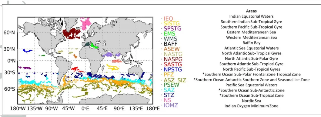
global ocean used in the present study are partitioned into 18 areas (Figure 1). The dataset of Chl and bbp here used, represents the update version of the databases BOPAD-prof and
is the depth where PAR reaches 1% of its surface value, was estimated from the Chl profile through the iterative process described in Morel and Maritorena (2001). Subsequently, the first optical depth, Zpd (units of m), was calculated as Zeu/4.6 (Morel, 1988). Finally, for each
profile, the mean and standard deviation of Chl and bbp were calculated within: i) the surface
layer: the layer between sea surface and the first optical depth; ii) the euphotic layer: the layer between sea surface and euphotic zone; and iii) the bottom layer: the layer between 950 and 1000 m.
2.2 𝒃𝒃𝒑𝒌 estimation: the model
In this study, the model developed by Brewin et al., (2012) is used to compute 𝑏𝑏𝑝𝑘 . The
bbp is modeled as a function of Chl and takes into account the fractional contributions of
small and large phytoplankton, as follows: 𝑏𝑏𝑝= 𝐶1𝑚·[𝑏
𝑏𝑝,1∗ − 𝑏𝑏𝑝,2∗ ][1 − 𝑒−𝑆1·Chl] + 𝑏𝑏𝑝,2∗ ·Chl + 𝑏𝑏𝑝𝑘 [1]
where the subscript 1 and 2 refer to two populations of phytoplankton cells partitioned according to size: 1 is for cells < 20𝜇m while 2 is for cells > 20𝜇m; 𝑏𝑏𝑝,1∗ and 𝑏
𝑏𝑝,2∗ refer to
the Chl-specific bbp coefficients associated with environments dominated by the two
populations of phytoplankton; 𝐶1𝑚 and 𝑆
1 refer to the maximum Chl concentration population
1 can reach and the initial slope relating the Chl concentration of population 1 to total Chl, respectively. The term 𝑏𝑏𝑝𝑘 refers to the background b
bp coefficient. The general equation of
the model can be simplified as:
𝑏𝑏𝑝 = 𝑐 · [1 − 𝑒(−𝑆1𝐶ℎ𝑙)] + 𝑏𝑏𝑝,2∗ · Chl + 𝑏𝑏𝑝𝑘 , [2]
in which 𝑏𝑏𝑝,2∗ is the slope, 𝑏𝑏𝑝𝑘 is the intercept of the fit, while c = 𝐶1𝑚[𝑏𝑏𝑝,1∗ − 𝑏𝑏𝑝,2∗ ]
and 𝑆1terms are the coefficients of the non-linear part of the model. The 𝑏𝑏𝑝,2∗ , 𝑏
𝑏𝑝𝑘 , c and
𝑆1coefficients are found from fitting Eq. 2 to bbp and Chl data by using the iterative bi-square
method (see paragraph 2.3). The initial guess for the four parameters are reported in Table S1. These values are in the range and order of magnitude of the values reported in Brewin et al., (2012). This model reduces to the Be05, Blc16 and Blc18 linear models if the non-linear term is discarded out, which would be the case where 𝑏𝑏𝑝,1∗ and 𝑏
𝑏𝑝,2∗ tend to the same value.
This model represents an evolution of the previous published model (i.e. Be05, Blc16 and Blc18) because of it takes into account the phytoplankton populations variability in the Chl-bbp relationship and thus for 𝑏𝑏𝑝𝑘 estimations. In addition, the inclusion of the non-linear term
introduces more flexibility reducing the fit errors for the areas here analyzed (see Figures S1 and S2).
The Eq. 2 is applied to each area (spatially-resolved with the temporal aggregation approach reported in Figure 1), and for every month (spatially- and temporal-resolved approach) for the two layers.
The ratio between the 𝑏𝑏𝑝𝑘 value found in the surface and in the bottom layers, and
analogously for the euphotic layer, enables understanding the difference between upper and deeper layers for each area of interest. It is computed as:
𝑏̂ =𝑏𝑝𝑘 𝑏𝑏𝑝,𝑠𝑢𝑟𝑓𝑎𝑐𝑒
𝑘
𝑏𝑏𝑝,𝑏𝑜𝑡𝑡𝑜𝑚𝑘 [3a]
𝑏
̂ =
𝑏𝑝𝑘 𝑏𝑏𝑝,𝑒𝑢𝑝ℎ𝑜𝑡𝑖𝑐𝑘𝑏𝑏𝑝,𝑏𝑜𝑡𝑡𝑜𝑚𝑘 [3b]
In addition to this ratio, 𝑏̅̅̅̅𝑏𝑝𝑘 is here defined as the fraction of the 𝑏
𝑏𝑝𝑘 with respect to the
median bbp (in %) giving an understanding on the relationship between NAP and particle
biomass in the different areas, and the layers, of the ocean:
𝑏𝑏𝑝𝑘
̅̅̅̅ =𝑏𝑏𝑝𝑘
𝑏𝑏𝑝 [4]
2.3 Model fit and statistics
For all the computations, Chl measurements below the value of 0.01 mg m-3 are considered too noisy for a proper estimation of 𝑏𝑏𝑝𝑘 and are filtered out from the dataset. The
model in Eq. 2 is fitted to the data using the iterative bi-square method which minimizes a weighted sum of squared errors, where the weight given to each data point decreases with the distance from the fitted curve (Huber, 1981). Therefore, the error function is sensitive to the bulk of the data and the effect of outliers is thus reduced. This error function is minimized through the Trust-Region algorithm (Moré and Sorensen, 1983) and the final fit estimate is found after a maximum of 400 iterations. For each 𝑏𝑏𝑝𝑘 the 95% confidence intervals and
two-standard deviation as confidence limit (2σ) are computed. In order to assess the model performance for the 𝑏𝑏𝑝𝑘 calculation, the root mean square (RMS; in m-1
) error between the modeled-bbp and measured-bbp are computed. The RMS is calculated according to:
𝑅𝑀𝑆 = √1
𝑁 ∑ (𝑏𝑏𝑝,𝑚𝑜𝑑𝑒𝑙𝑒𝑑,𝑖 −𝑏𝑏𝑝,𝑚𝑒𝑎𝑠𝑢𝑟𝑒𝑑,𝑖)
2 𝑁
𝑖=1
3.
Results and Discussion
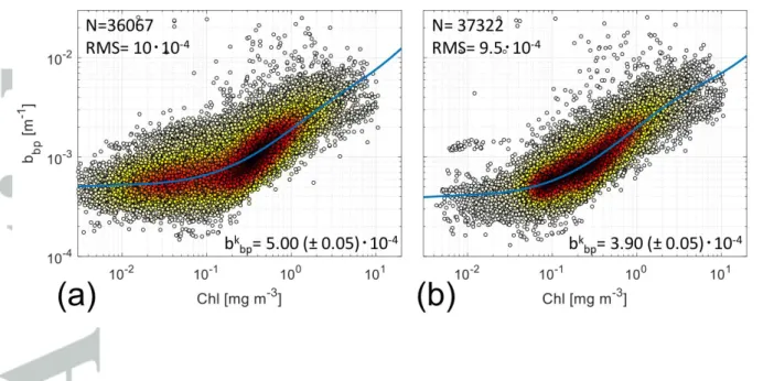
3.1 Global overview of 𝑏𝑏𝑝𝑘Aggregated quality-controlled data within the surface layer for all areas and months (N=36067) are shown in Figure 2a. The bbp coefficients increase with Chl but with relatively
constant bbp for low Chl values (Figure 2a). This behavior is consistent with previous
observations by Behrenfeld et al. (2005) and Brewin et al. (2012), and is considered to be the consequence of two distinct oceanic conditions: “photoacclimation-dominance” and “biomass-dominance” of Chl signal. The former is typical of oligotrophic areas (e.g. subtropical gyres) where variability of Chl is uncoupled with biomass and the process of acclimation to light and nutrients drives Chl variations (Siegel et al., 2013; Halsey and Jones, 2015; Barbieux et al., 2018). On the reverse, the latter case is typical of most productive areas where Chl and bbp strongly covary(Dall’Olmo et al., 2009, 2012; Westberry et al., 2010). The
high Chl-bbp co-variability is a clear indication that particles (and biomass) covary with
phytoplankton abundance, while the physiological photoacclimation process playing a secondary role in determining the Chl variations.
Here, the application of the Br12 model to these BGC-Argo data leads to a 𝑏𝑏𝑝𝑘 equal to
5.0·10-4 m-1 at the surface, a value higher than that found by Be05 (3.5·10-4 m-1 at 443 nm). On the other hand, Br12 reported 7.0·10-4 m-1 for 470 nm and 5.6·10-4 m-1 at 526 nm. Blc18 found a median 𝑏𝑏𝑝𝑘 value equal to 9.5·10-4
m-1 based on 19-years of ocean colour data. These values are comparable as the spectral variability is limited in case of bbp (±30% between
443nm and 700nm when assuming bbp decreasing as a power law with slope equal to 0.7). In
relative terms, our study shows that 𝑏𝑏𝑝𝑘 dominate within the surface layer as it accounts for
57% of the total bbp measured by all BGC-Argo floats, a remarkably high percentage.
An increased Chl-bbp co-variability is observed within the euphotic layer (Figure 2b;
N=37322). The derived 𝑏𝑏𝑝𝑘 is not comparable to our estimates from the surface layer or from previous satellite observations because it includes deeper layers where there is high particle concentration, as for example oligotrophic areas such as the subtropical gyres and the eastern Mediterranean Sea (Volpe et al., 2007; Barbieux et al., 2018). The first estimation of 𝑏𝑏𝑝𝑘 for
this layer is a value of 3.9·10-4 m-1, and accounts for 45% of the total bbp, suggesting that in
the euphotic layer NAP are more correlated to Chl than at the surface.
3.2 Geographical distribution of 𝑏𝑏𝑝𝑘
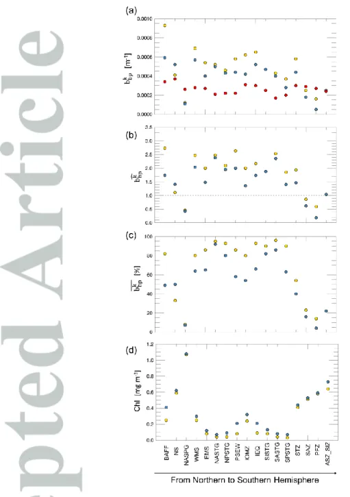
Figure 3a shows 𝑏𝑏𝑝𝑘 estimations for the surface, euphotic and bottom layers within
each geographical area sampled by BGC-Argo floats. In surface layer, the range of variability spans between 10-4 m-1 and 10-3 m-1, consistent with global ocean-colour estimations (Bellacicco et al., 2018). Lower variability characterizes the euphotic layer (of a factor of ~6), from ~1.0·10-4 m-1 to 6.0·10-4 m-1. For the bottom layer, variability is the lowest, between 2.0·10-4 m-1 and 4.0·10-4 m-1. The two upper layers display a latitudinal gradient, with a general 𝑏𝑏𝑝𝑘 decrease from northern to southern oceans. 𝑏
𝑏𝑝𝑘 in the bottom layer does not show
a clear geographical pattern and remains relatively constant across all sampled oceanic areas. Figure 3b shows the 𝑏̂𝑏𝑝𝑘 for each area, the ratios between the spatially-resolved 𝑏
𝑏𝑝𝑘
found at the surface and euphotic layers with the estimation for the bottom layer. Globally, 𝑏̂𝑏𝑝𝑘 is higher in the upper layer than the at the bottom from mid- to low-latitudes, while 𝑏
𝑏𝑝𝑘 at
the bottom is higher than at the surface in most productive seas such as the NASPG, SAZ, PFZ and ASZ_SIZ areas (Uitz et al., 2009; Alkire et al., 2014; Artega et al., 2018). In these
areas, 𝑏̅̅̅̅𝑏𝑝𝑘 is only a small fraction of the total b
bp in surface waters (< 20%; Figure 3c) as a
consequence of the higher relative variability in the bbp and phytoplankton abundance (Alkire
et al., 2014). In the NASPG, characterized by high phytoplankton biomass, 𝑏̅̅̅̅𝑏𝑝𝑘 is lower than
10%. It means that bbp is more dominated by particles that covary with phytoplankton cells
(see Eq. 1), thus being more influenced by phytoplankton dynamics.
In the Southern Ocean (i.e. STZ, SAZ, PFZ and ASZ_SIZ areas), 𝑏̅̅̅̅𝑏𝑝𝑘 ranges from 15% (i.e.
PFZ) to 60% (i.e. STZ) for surface waters suggesting inorganic particles (e.g. coccoliths) can also drive the 𝑏𝑏𝑝𝑘 signal (Figure 3c). Indeed, coccoliths concentrations covary with bbp
because they scatter light with high efficiency (Balch et al. 2016; 2018). The 𝑏𝑏𝑝𝑘 values, and their order of magnitude, are consistent with measurements of bbp from CaCO3 reported in
Balch et al. (2016) along the Great Calcite Belt (GCB) (their Figure 2c). Thus, in these areas of the Southern Ocean, the 𝑏𝑏𝑝𝑘 may be related to the coccolithophorids seasonality (i.e. skeleton compounds of no longer living cells; 𝑏𝑏𝑝𝑘 is the b
bp when Chl is zero) (Balch et al.
2016; 2018; Bellacicco et al., 2018).
In less productive areas (e.g. EMS, IEQ, NASTG, SISTG, SASTG, SPSTG; Figure 3d), 𝑏𝑏𝑝𝑘
̅̅̅̅ is greater than 80% at the surface layer, consistent with previous findings (Brewin et al., 2012; Bellacicco et al., 2018). These areas are characterized by limited nutrients availability determining low phytoplankton biomass, especially pico- and nano-phytoplankton dominated communities (Bricaud et al., 2004; Mignot et al., 2014), which are rapidly recycled in the surface layer thus supporting relatively high bacterial and detrital biomass. For the euphotic layer, much of the bbp can be related to phytoplankton biomass as highlighted by a lower 𝑏̅̅̅̅𝑏𝑝𝑘
value of around 60%. This is the consequence of the subsurface chlorophyll maximum (SCM) which is deeper in the subtropical gyres and oligotrophic seas as found by Mignot et al., (2014) and Barbieux et al., (2019). It determines that, at depth, there is an increase of phytoplankton biomass and of NAP covarying with phytoplankton: the 𝑏𝑏𝑝𝑘 coefficient indeed
decreases from the surface to the euphotic layers (Figure 3a).
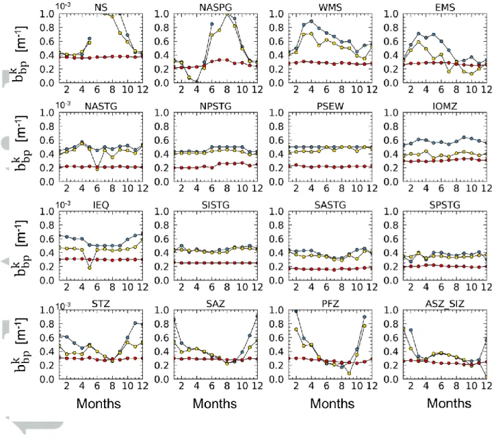
3.3 Seasonal variability of 𝑏𝑏𝑝𝑘
The 𝑏𝑏𝑝𝑘 values within surface and euphotic layers show a clear seasonal cycle with
maxima during the productive periods (𝑏𝑏𝑝𝑘 > 5.0·10-4
) and minima during the low productive periods (𝑏𝑏𝑝𝑘 < 4.0·10-4
) in all the areas outside the oligotrophic seas (e.g. NS, NASPG, WMS, EMS, STZ, SAZ, PFZ, ASZ_SIZ) (Figure 4).
In the NASPG, 𝑏𝑏𝑝𝑘 shows high values during the well-known spring bloom and low values from December to April (Briggs et al., 2011; Alkire et al., 2014; Mignot et al., 2018). In the Southern Ocean, and especially SAZ, PFZ and ASZ_SIZ areas, 𝑏𝑏𝑝𝑘 shows the maxima
values from December to April (i.e. period of bloom) while the minima are detected in the period May-September.
In the Mediterranean Sea (i.e. WMS and EMS), the seasonal cycle varies within the sub-basins showing different amplitude and shape, clearly linked to the regional trophic
regimes. WMS shows 𝑏𝑏𝑝𝑘 values higher than the eastern ones confirming the presence of a
general decreasing eastward gradient for this coefficient. In the western basin of Mediterranean Sea, deep-water formation dynamics and/or the generally shallow nutricline results in a maximum value in April. On the contrary, maxima generally occur earlier between February and March in the eastern Mediterranean basin. These results confirm Bellacicco et al., (2016) findings for this semi-enclosed basin. In their work, 𝑏𝑏𝑝𝑘 was demonstrated to be variable both in space and time with a marked seasonality in the different bio-regions of both the sub-basins. As shown by Bellacicco et al., (2016), periods characterized by lower 𝑏𝑏𝑝𝑘 (e.g. summer) are also associated with higher variability and uncertainties in the estimations. This is valid for the 𝑏𝑏𝑝𝑘 both in the surface and euphotic layers, and has to be taken into account in the interpretation of these results (see Tables S3 and S4).
The 𝑏𝑏𝑝𝑘 at the bottom layer shows a smoother seasonal cycle in respect to what occur
in the upper layers. As found by Poteau et al., (2017), an annual cycle is only observed at the Southern Ocean and sub-polar North Atlantic area, regions with the largest amplitude in the seasonal cycles at the surface and euphotic layer (Figure 4) due to blooms of large phytoplankton (Alkire et al., 2014; Barbieux et al., 2018). Poteau et al., (2017), indeed, suggested that the 𝑏𝑏𝑝𝑘 at the depth can be mostly related to disaggregation of these large
settling particles.
The seasonal cycle of 𝑏𝑏𝑝𝑘 in the less productive seas for all the layers is low, suggesting
low NAP seasonal variations (e.g. detrital matter, heterotrophic bacteria, virus). The 𝑏𝑏𝑝𝑘
estimation for each month appears to be nearly constant throughout the year (Figure 4) and thus bbp may be controlled mostly by 𝑏𝑏𝑝𝑘 , as highlighted also in Figure 3c.
4.
Conclusions
In this work, an extensive global dataset of Chl and bbp (700) measurements acquired
from Biogeochemical-Argo (BGC-Argo) profiling floats was analyzed. Specifically, we investigated and describe the spatial, vertical and temporal variability of 𝑏𝑏𝑝𝑘 at global scale.
The main results are:
o 𝑏𝑏𝑝𝑘 shows a similar order of magnitude in both surface and euphotic layers, as previously published works based on ocean-colour data: ranging between 10-4 and 10-3 m-1.
o In the surface layer, the 𝑏𝑏𝑝𝑘 increase from southern to the northern hemisphere,
confirming what was found by Bellacicco et al., (2018) using ocean-colour data.
o In the surface layer of most productive areas (e.g. NASPG), the 𝑏𝑏𝑝𝑘 is only a small
fraction of the total bbp (< 20%), while in the oligotrophic waters, 𝑏𝑏𝑝𝑘 is the main
contributor to the total bbp (> 80%). In the euphotic layer of the oligotrophic areas, the 𝑏𝑏𝑝𝑘
o In the surface and euphotic layers, the 𝑏𝑏𝑝𝑘 shows strong seasonal variability in the main
productive areas of the global ocean, such as NASPG and the Southern Ocean areas. 𝑏𝑏𝑝𝑘
has instead a weak temporal variability in the low productivity areas, such as the subtropical gyres. This is valid also for the 𝑏𝑏𝑝𝑘 estimations at the bottom layer.
The 𝑏𝑏𝑝𝑘 is a key parameter for satellite estimations of phytoplankton biomass in terms of carbon (Behrenfeld et al., 2005, 2016; Bellacicco et al., 2016, 2018, 2019; Martinez-Vicente et al., 2017; Westberry et al., 2008, 2016). Recently, Bellacicco et al., (2018) highlighted the difference (of around a factor of 2) in the phytoplankton carbon biomass estimation from space by using a 𝑏𝑏𝑝𝑘 variable in space, rather than a single value. Consequently, inclusion of this reported spatial-temporal and depth variations of 𝑏𝑏𝑝𝑘 into
phytoplankton carbon models may help to improve their predictions from remote sensing data (Martinez-Vicente et al., 2017) but also from BGC-Argo floats (Mignot et al., 2014, 2018).
Remote optical-based predictions and interpretation of phytoplankton carbon models would also benefit from a better understanding of NAP composition and which particles generate the bbp signal across the world’s oceans. Indeed, submicron detrital particles have
long been considered as the main source of bbp (Stramski et al., 2004). However, Organelli et
al. (2018) has highlighted that bbp is mainly due to particles with diameters between 1-10 μm
which may also include NAP and aggregates. This latter study thus opens the way to new questions on the sources of the open-ocean bbp signal that are critical to improving our
interpretation of open-ocean bbp.
Future research challenges should therefore be directed to: (i) understand the drivers of the observed spatio-temporal variability and explore the composition of NAP across the world’s oceans and how it influences the bbp and 𝑏𝑏𝑝𝑘 signal; (ii) study the impact on
biogeochemistry of 𝑏𝑏𝑝𝑘 , e.g. on the particles assemblage in different ocean trophic regimes (i.e. subpolar, subtropical); (iii) include 𝑏𝑏𝑝𝑘 spatial and temporal variability into phytoplankton carbon estimations from space and its connections with phytoplankton physiology; and most importantly (iv): advance technology for (autonomous) optical measurements of NAP directly, for example by exploiting the birefringence properties of mineral particles such as calcite compounds (Guay and Bishop, 2002; Bishop and Wood, 2009), and acquire spectral angular scattering to better understand the influence of bubbles and plastics (Zhang et al., 1998; Twardowski et al., 2012).
Acknowledgements
M. Bellacicco conceived this work during his stays at the Laboratoire d’Oceanographie de Villefranche sur Mer (LOV) supported by a postdoctoral fellowship of the Centre Nationales
d’Etudes Spatiales (CNES; France). Currently, M. Bellacicco has a postdoctoral fellowship by the European Space Agency (ESA). This work was supported by the ESA Living Planet Fellowship
Project PHYSIOGLOB: Assessing the inter-annual physiological response of phytoplankton to global warming using long-term satellite observations, 2018-2020.
The paper is also a contribution to the following research projects: remOcean (funded by the European Research Council, grant 246777), NAOS (funded by the Agence Nationale de la Recherche in the frame of the French ‘‘Equipement d’avenir’’ program, grant ANR J11R107-F), SOCLIM
(Southern Ocean and climate) project supported by the French research program LEFECYBER of INSU-CNRS, the Climate Initiative of the foundation BNP Paribas and the French polar institute (IPEV), AtlantOS (funded by the European Union’s Horizon 2020 Research and Innovation program, grant 2014– 633211), E-AIMS (funded by the European Commission’s FP7 project, grant 312642), U.K. Bio-Argo (funded by the British Natural Environment Research Council—NERC, grant NE/ L012855/1), REOPTIMIZE (funded by the European Union’s Horizon 2020 Research and Innovation program, Marie Skłodowska-Curie grant 706781 assigned to E. Organelli), Argo-Italy (funded by the Italian Ministry of Education, University and Research - MIUR), and the French Bio-Argo program (BGC-Argo France; funded by CNES-TOSCA, LEFE Cyber, and GMMC).
All the BGC-Argo data are available at the Coriolis database (ftp://ftp.ifremer.fr/ifremer/argo/dac/coriolis).
References
1. Alkire, M. B., Lee, C., D’Asaro, E., Perry, M. J., Briggs, N., Cetinić, I., & Gray, A. (2014). Net community production and export from Seaglider measurements in the North Atlantic after the spring bloom. Journal of Geophysical Research: Oceans, 119, 6121– 6139. https://doi.org/10.1002/2014JC010105
2. Antoine, D., Siegel, D. A., Kostadinov, T., Maritorena, S., Nelson, N. B., Gentili, B., ... & Guillocheau, N. (2011). Variability in optical particle backscattering in contrasting bio‐ optical oceanic regimes. Limnology and Oceanography, 56(3), 955-973.
3. Arteaga, L., Haëntjens, N., Boss, E., Johnson, K. S., & Sarmiento, J. L. (2018). Assessment of export efficiency equations in the Southern Ocean applied to satellite‐ based net primary production. Journal of Geophysical Research: Oceans, 123(4), 2945-2964
4. Azam, F., Fenchel, T., Field, J. G., Grey, J. S., Meyer-Reil, L. A., & Thingstad, F. (1983). The ecological role of water-column microbes. Mar. ecol. Prog. ser, 10, 257-263.
5. Balch, W. M., Bates, N. R., Lam, P. J., Twining, B. S., Rosengard, S. Z., Bowler, B. C., ... & Rauschenberg, S. (2016). Factors regulating the Great Calcite Belt in the Southern Ocean and its biogeochemical significance. Global Biogeochemical Cycles, 30(8), 1124-1144.
6. Balch, W. M. (2018). The ecology, biogeochemistry, and optical properties of coccolithophores. Annual review of marine science, 10, 71-98.
7. Barbieux, M., Uitz, J., Bricaud, A., Organelli, E., Poteau, A., Schmechtig, C., ... & D'Ortenzio, F. (2018). Assessing the Variability in the Relationship Between the Particulate Backscattering Coefficient and the Chlorophyll a Concentration from a Global Biogeochemical‐Argo Database. Journal of Geophysical Research: Oceans, 123(2), 1229-1250.
8. Behrenfeld, M. J., Boss, E., Siegel, D. A., & Shea, D. M. (2005). Carbon‐based ocean productivity and phytoplankton physiology from space. Global biogeochemical cycles, 19(1).
9. Behrenfeld, M. J., O’Malley, R. T., Boss, E. S., Westberry, T. K., Graff, J. R., Halsey, K. H., ... & Brown, M. B. (2016). Revaluating ocean warming impacts on global phytoplankton. Nature Climate Change, 6(3), 323.
10. Bellacicco, M., Volpe, G., Colella, S., Pitarch, J., & Santoleri, R. (2016). Influence of photoacclimation on the phytoplankton seasonal cycle in the Mediterranean Sea as seen by satellite. Remote Sensing of Environment, 184, 595-604.
11. Bellacicco, M., Volpe, G., Briggs, N., Brando, V., Pitarch, J., Landolfi, A., ... & Santoleri, R. (2018). Global Distribution of Non‐Algal Particles From Ocean Color Data and
Implications for Phytoplankton Biomass Detection. Geophysical Research Letters, 45(15), 7672-7682.
12. Bellacicco, M., Vellucci, V., Scardi, M., Barbieux, M., Marullo, S., & D’Ortenzio, F. (2019). Quantifying the Impact of Linear Regression Model in Deriving Bio-Optical Relationships: The Implications on Ocean Carbon Estimations. Sensors, 19(13), 3032. 13. Bishop, J. K., & Wood, T. J. (2009). Year‐round observations of carbon biomass and flux
variability in the Southern Ocean. Global Biogeochemical Cycles, 23(2).
14. Brewin, R. J., Dall’Olmo, G., Sathyendranath, S., & Hardman-Mountford, N. J. (2012). Particle backscattering as a function of chlorophyll and phytoplankton size structure in the open-ocean. Optics express, 20(16), 17632-17652.
15. Bricaud, A., Babin, M., Claustre, H., Ras, J., & Tièche, F. (2010). Light absorption properties and absorption budget of Southeast Pacific waters. Journal of Geophysical Research, 115, C08009. https://doi.org/10.1029/2009JC005517.
16. Briggs, N., Perry, M. J., Cetinić, I., Lee, C., D'Asaro, E., Gray, A. M., & Rehm, E. (2011). High-resolution observations of aggregate flux during a sub-polar North Atlantic spring bloom. Deep Sea Research Part I: Oceanographic Research Papers, 58(10), 1031-1039. 17. Cho, B. C., & Azam, F. (1990). Biogeochemical significance of bacterial biomass in the
ocean's euphotic zone. Marine ecology progress series. Oldendorf, 63(2), 253-259
18. Dall'Olmo, G., Westberry, T. K., Behrenfeld, M. J., Boss, E., & Slade, W. H. (2009). Direct contribution of phytoplankton-sized particles to optical backscattering in the open ocean. Biogeosciences Discussions, 6(1).
19. Dall’Olmo, G., Boss, E., Behrenfeld, M. J., & Westberry, T. K. (2012). Particulate optical scattering coefficients along an Atlantic Meridional Transect. Optics express, 20(19), 21532-21551.
20. Gray, A. R., Johnson, K. S., Bushinsky, S. M., Riser, S. C., Russell, J. L., Talley, L. D., ... & Sarmiento, J. L. (2018). Autonomous Biogeochemical Floats Detect Significant Carbon Dioxide Outgassing in the High‐ Latitude Southern Ocean. Geophysical Research Letters, 45(17), 9049-9057.
21. Guay, C. K., & Bishop, J. K. (2002). A rapid birefringence method for measuring suspended CaCO3 concentrations in seawater. Deep Sea Research Part I: Oceanographic Research Papers, 49(1), 197-210.
22. Halsey, K. H., & Jones, B. M. (2015). Phytoplankton strategies for photosynthetic energy allocation. Annual review of marine science, 7, 265-297.
23. Huber, P. J. (1981). Robust Statistics. Hoboken, NJ: John Wiley & Sons, Inc.
24. Martínez-Vicente, V., Evers-King, H., Roy, S., Kostadinov, T. S., Tarran, G. A., Graff, J. R., ... & Röttgers, R. (2017). Intercomparison of ocean color algorithms for picophytoplankton carbon in the ocean. Frontiers in Marine Science, 4, 378.
25. MATLAB and Statistics Toolbox, The MathWorks, Inc., Natick, Massachusetts, United States.
26. Mignot, A., Claustre, H., Uitz, J., Poteau, A., D'Ortenzio, F., & Xing, X. (2014). Understanding the seasonal dynamics of phytoplankton biomass and the deep chlorophyll maximum in oligotrophic environments: A Bio‐Argo float investigation. Global Biogeochemical Cycles, 28(8), 856-876.
27. Mignot, A., Ferrari, R., & Claustre, H. (2018). Floats with bio-optical sensors reveal what processes trigger the North Atlantic bloom. Nature communications, 9(1), 190.
28. Moré, J. J., & Sorensen, D. C. (1983). Computing a trust region step. SIAM Journal on Scientific and Statistical Computing, 4(3), 553-572.
29. Morel, A. (1988). Optical modeling of the upper ocean in relation to its biogenous matter content (case I waters). Journal of geophysical research: oceans, 93(C9), 10749-10768.
30. Morel, A., & Ahn, Y. H. (1990). Optical efficiency factors of free-living marine bacteria: Influence of bacterioplankton upon the optical properties and particulate organic carbon in oceanic waters. Journal of Marine Research, 48(1), 145-175.
31. Morel, A., & Ahn, Y. H. (1991). Optics of heterotrophic nanoflagellates and ciliates: A tentative assessment of their scattering role in oceanic waters compared to those of bacterial and algal cells. Journal of Marine Research, 49(1), 177-202.
32. Morel, A., & Maritorena, S. (2001). Bio‐optical properties of oceanic waters: A reappraisal. Journal of Geophysical Research: Oceans, 106(C4), 7163-7180.
33. Organelli, E., Barbieux, M., Claustre, H., Schmechtig, C., Poteau, A., Bricaud, A., ... & Leymarie, E. (2017). Two databases derived from BGC-Argo float measurements for marine biogeochemical and bio-optical applications. Earth System Science Data, 9, 861-880.
34. Organelli, E., Dall’Olmo, G., Brewin, R. J., Tarran, G. A., Boss, E., & Bricaud, A. (2018). The open-ocean missing backscattering is in the structural complexity of particles. Nature Communications, 9(1), 5439.
35. Poteau, A., Boss, E., & Claustre, H. (2017). Particulate concentration and seasonal dynamics in the mesopelagic ocean based on the backscattering coefficient measured with Biogeochemical‐ Argo floats. Geophysical Research Letters, 44(13), 6933-6939.
36. Siegel, D. A., Behrenfeld, M. J., Maritorena, S., McClain, C. R., Antoine, D., Bailey, S. W., ... & Eplee Jr, R. E. (2013). Regional to global assessments of phytoplankton dynamics from the SeaWiFS mission. Remote Sensing of Environment, 135, 77-91. 37. Siokou-Frangou, I., Christaki, U., Mazzocchi, M. G., Montresor, M., Ribera d’Alcalà, M.,
Vaqué, D., & Zingone, A. (2010). Plankton in the open Mediterranean Sea: a review. 38. Sosik. H. M. Characterizing seawater constituents from optical properties. In M. Babin,
C. S. Roesler and J. J. Cullen [eds.]. Real-time coastal observing systems for ecosystem dynamics and harmful algal blooms. UNESCO, pp. 281-329. (peer reviewed) (2008). 39. Stramski, D., & Kiefer, D. A. (1991). Light scattering by microorganisms in the open
ocean. Progress in Oceanography, 28(4), 343-383.
40. Stramski, D., Boss, E., Bogucki, D., & Voss, K. J. (2004). The role of seawater constituents in light backscattering in the ocean. Progress in Oceanography, 61(1), 27-56. 41. Twardowski, M., Zhang, X., Vagle, S., Sullivan, J., Freeman, S., Czerski, H., ... & Kattawar, G. (2012). The optical volume scattering function in a surf zone inverted to derive sediment and bubble particle subpopulations. Journal of Geophysical Research: Oceans, 117(C7).
42. Uitz, J., Claustre, H., Griffiths, F. B., Ras, J., Garcia, N., & Sandroni, V. (2009). A phytoplankton class-specific primary production model applied to the Kerguelen Islands region (Southern Ocean). Deep Sea Research Part I: Oceanographic Research Papers, 56(4), 541-560.
43. Volpe, G., Santoleri, R., Vellucci, V., d'Alcalà, M. R., Marullo, S., & d'Ortenzio, F. (2007). The colour of the Mediterranean Sea: Global versus regional bio-optical algorithms evaluation and implication for satellite chlorophyll estimates. Remote Sensing of Environment, 107(4), 625-638.
44. Westberry, T., Behrenfeld, M. J., Siegel, D. A., & Boss, E. (2008). Carbon‐based primary productivity modeling with vertically resolved photoacclimation. Global Biogeochemical Cycles, 22(2).
45. Westberry, T. K., Dall’Olmo, G., Boss, E., Behrenfeld, M. J., & Moutin, T. (2010). Coherence of particulate beam attenuation and backscattering coefficients in diverse open ocean environments. Optics Express, 18(15), 15419-15425.
46. Westberry, T. K., Schultz, P., Behrenfeld, M. J., Dunne, J. P., Hiscock, M. R., Maritorena, S., ... & Siegel, D. A. (2016). Annual cycles of phytoplankton biomass in the subarctic Atlantic and Pacific Ocean. Global Biogeochemical Cycles, 30(2), 175-190. 47. Zhang, X., Lewis, M., & Johnson, B. (1998). Influence of bubbles on scattering of light in
Figure 1: Geographical distribution of the BGC-Argo dataset on a global ocean scale. Each colour represents sampling areas and abbreviations. * indicates data acquired in four regions below 30°S which have been delineated by using temperature profiles (Gray et al., 2018): Sub-Tropical Zone (STZ) with a temperature at 100 m above 11°C; the Sub-Antarctic Zone (SAZ) with a temperature at 400 m below 5°C; the Polar Frontal Zone (PFZ) with the minimum temperature between 0 and 200 m above 2°C; the Antarctic Southern Zone and Seasonal Ice Zone (ASZ_SIZ) minimum temperature between 0 and 200 m below 2°C.
Figure 2: Plot density between Chl and bbp (700) within the surface layer (panel a) and the euphotic
layer (panel b). Both panels include the number of observations (N) and the RMS (in m-1). The 𝑏𝑏𝑝𝑘 estimation (in m-1) with two standard deviation as confidence limit (2) is also reported. Chl
values < 0.01 mg m-3 are not included in the fit computations. The plots are presented in logarithmic scale in both axes though the fit has been calculated in linear scale. Dot density is indicated as color from white (low density) to black (high density).
Figure 3: Geographical distribution of 𝑏𝑏𝑝𝑘 (in m-1
) in the three layers: surface (gold), euphotic (blue) and bottom (red) (a). The 𝑏̂𝑏𝑝𝑘 for the surface (gold) and euphotic (blue) layers for each area (b). The
dashed line indicates the case where 𝑏̂𝑏𝑝𝑘 estimates between surface or euphotic layer with bottom
layer are close to the same value. Panel c shows the 𝑏̅̅̅̅̅ (in %) for each area and layer (gold for 𝑏𝑝𝑘
surface layer; blue for euphotic layer). The model performance, in terms of RMS (m-1) and interval of confidence at 95% for each 𝑏𝑏𝑝𝑘 estimation is reported in the supplementary information (see Figures
S3, S4; Table S2). ASEW area is not included in this analysis due to the low performance of the model and highest uncertainties in 𝑏𝑏𝑝𝑘 assessment in both layer (for details see the supplementary materials). Note that the areas have been sorted from the northern to the southern hemisphere. Panel d shows the mean Chl values for each region and layers (gold for surface layer and blue for euphotic layer). See Table 1 for locations and abbreviations.
Figure 4: Temporal variability of 𝑏𝑏𝑝𝑘 (in m-1
) for each area and all the three layers: surface (gold), euphotic (blue) and bottom (red). The model performance, in terms of RMS (m-1) and interval of confidence at 95% for each monthly 𝑏𝑏𝑝𝑘 estimation, are reported in the supplementary materials (see Tables S3, S4 and S5). ASEW and BAFF areas are not included in the analysis due to the absence/limited number of observations that prevents the description of the annual cycle. See Table 1 for locations and abbreviations.