Testing unilateral and bilateral link formation

HAL Id: halshs-00574971

https://halshs.archives-ouvertes.fr/halshs-00574971

Preprint submitted on 9 Mar 2011

HAL is a multi-disciplinary open access archive for the deposit and dissemination of sci-entific research documents, whether they are pub-lished or not. The documents may come from teaching and research institutions in France or abroad, or from public or private research centers.

L’archive ouverte pluridisciplinaire HAL, est destinée au dépôt et à la diffusion de documents scientifiques de niveau recherche, publiés ou non, émanant des établissements d’enseignement et de recherche français ou étrangers, des laboratoires publics ou privés.

Testing unilateral and bilateral link formation

Margherita Comola, Marcel Fafchamps

To cite this version:

Margherita Comola, Marcel Fafchamps. Testing unilateral and bilateral link formation. 2009. �halshs-00574971�

WORKING PAPER N° 2009 - 30

Testing unilateral and bilateral link formation

Margherita Comola

Marcel Fafchamps

JEL Codes: C12, C52, D85

Keywords: network architecture, pairwise stability, risk

sharing

P

-

S

E

L

’E

A

-

48,BD JOURDAN –E.N.S.–75014PARIS TÉL. :33(0)143136300 – FAX :33(0)143136310

www.pse.ens.fr

Testing Unilateral and Bilateral Link Formation

Margherita Comolay

Paris School of Economics

Marcel Fafchampsz

Oxford University December 2009

Abstract

We propose a test of whether self-reported network data is best seen as an actual link or willingness to link and, in the latter case, whether this link is generated by an unilateral or bilateral link formation process. We illustrate this test using survey answers to a risk-sharing question in an African village. We …nd that bilateral link formation …ts the data better than unilateral link formation, but the data are best interpreted as willingness to link rather than an actual link. We then expand the model to include self-censoring and …nd it to …t the data signi…cantly better than willingness to link. This suggests that, in our data, the data generating process behind self-reported links is a hybrid between an actual link and willingness to link.

JEL codes: C12; C52; D85

Keywords: pairwise stability; self-reported link; self-censoring; risk sharing

We thank Michael Wooldridge for his useful suggestions and Joachim De Weerdt for making the data available. We have bene…tted from useful comments from Yann Bramoulé and from seminar participants at the Paris School of Economics, Oxford University, and the University of Nottingham.

y_{Paris School of Economics. Email: comola@pse:ens:fr}

1. Introduction

It is increasingly recognized that many important economic phenomena, such as trade, informa-tion di¤usion, and learning, take place within social networks (e.g. Granovetter 1985, Jackson 2008) and that the architecture of these networks can a¤ect the e¢ ciency and equity of the re-sulting allocation (Vega-Redondo 2006). We also now know that the mechanism through which links are created has a profound in‡uence on the equilibrium architecture of purposely formed networks. In particular, Bala and Goyal (2000) have shown that unilateral and bilateral link formation result in fundamentally di¤erent network structures – see also Goyal (2007). The consent rule (unilateral versus bilateral) within a group may also shape the aggregate outcome, as Charness and Jackson (2007) have shown in an experimental set-up.

Bilateral link formation refers to situations in which the consent of both nodes is needed for a link to be formed; it is a natural assumption for voluntary exchange. Unilateral link formation arises whenever one node can form a link without the express consent of the other; it is a natural assumption for information access networks, e.g., the Internet. It may also arise in market exchange when legal or social norms make it unlawful for one party to refuse to trade.1

The contribution of this paper is primarily methodological. The econometric analysis of social networks is still novel, and there often is a lack of clarity on the implicit assumptions necessary to estimate network models. The ultimate aim of this paper is to shed some light on the way self-reported network data should be interpreted, and how discordant responses should be treated. We …nd that in our case some models …t the data better than others. Other data may yield di¤erent conclusions.

We propose a simple methodology for testing whether self-reported network data re‡ect a

1_{In many developed countries anti-discrimination laws typically make it unlawful for a retailer to refuse to sell}

simple willingness to link or an existing link and, in the latter case, whether this link is gen-erated by an unilateral or bilateral link formation process. Building on the work of Comola (2007), we take pairwise stability as starting point for the estimation process. First introduced by Jackson and Wolinsky (1996), pairwise stability has established itself as a cornerstone equi-librium condition in the study of bilateral link formation processes (Goyal 2007). Using pairwise stability as starting point, Comola (2007) uses a bivariate probit model to estimate a bilateral link formation model. We extend this approach by noting that, under unilateral link formation, the absence of a link is formally equivalent to a pairwise stable decision by both nodes not to form a link.

We illustrate our methodology using data on self-reported mutual insurance links. This is a natural choice given that many empirical studies of social networks have relied on self-reported data and that mutual insurance networks have received much attention in the literature (e.g. Scott 1976, Altonji, Hayashi and Kotliko¤ 1992, Coate and Ravallion 1993, Townsend 1994, Fafchamps and Lund 2003). Every household in an African village was asked to give a list of households on whom they rely – or who rely on them – for help in cash, kind or labor. The question is intended to capture a link between two households i and j and should in principle be answered in the same way by both, irrespective of whether the assistance is one-sided or reciprocated. In practice, it is frequent that household i mentions j but j does not mention i.

This is open to multiple interpretations. One possibility is that respondents gave the names of households from whom they wish to seek assistance, not necessarily those who would provide it, should the need arise. In this case, answers are best understood as representing willingness to link, not an actual link. Another interpretation is that respondents provided information on actual links but their answers di¤er because of misreporting. It is unclear a priori which of these two alternatives is a better representation of the data.

To test between the two, we use the fact that actual links should satisfy equilibrium condi-tions; willingness to link need not. Two types of equilibrium conditions are considered, depending on whether link formation is bilateral or unilateral. It seem natural to expect mutual insurance links to require the agreement of both parties – and this is indeed how the economic literature has modeled informal risk sharing (e.g. Coate and Ravallion 1993, Kocherlakota 1996). In this case, link formation is bilateral and pairwise stability is a necessary condition for the network to be in equilibrium.2

It is also conceivable that social norms make it impossible for villagers to refuse assisting others. For instance, a son may not be able to refuse helping his father. Platteau (1996) argues that many agrarian societies, especially in sub-Saharan Africa, cultivate egalitarian norms, a point that has repeatedly been made by anthropologists and by casual observers alike.3 In the

presence of sharing norms, the link formation process is basically unilateral. In this case, a transformed version of the pairwise stability condition must hold in the sense that both nodes must agree not to form a link.

Comola (2007) has shown that, under the normality assumption, the restrictions imposed by pairwise stability take the form of a bilateral probit model with partial observability (Poirier 1980). In contrast, if answers only represent willingness to link, the relevant regression model is a simple probit. Building on this insight, we test whether willingness to link, bilateral, or unilateral link formation is most consistent with the responses given by surveyed households. This is achieved using the non-nested likelihood ratio test …rst proposed by Vuong (1989), that we adapt to correct for network dependence across residuals. When we peg the bilateral and unilateral models against each other, we …nd that the bilateral link formation model wins.

2_{Pairwise stability does not fully characterise equilibrium in the village network; it is a local condition. One}

could therefore argue that our test is not e¢ cient since it fails to impose all the structure of a village network equilibrium. The di¢ culty is that deriving global equilibria would require additional assumptions about the information each household has about all payo¤s, etc, something we are reluctant to do.

However, both are outperformed by a simple willingness-to-link model.

We then relax the willingness-to-link model to allow for self-censoring. For instance, a respondent i may refrain from reporting his wish to seek help from j if he anticipates rejection. Alternatively, i may report links with individuals who he cannot refuse to help even though he prefers not to. Both cases involve self-censoring –of willingness to link in the …rst case, and of unwillingness to link in the second. We show that self-censoring can be represented as a bilateral probit model without cross-equation coe¢ cient restrictions.

We …nd evidence of self-censoring in our data. This is important because self-censoring of reported willingness to link has long plagued the study of link formation (e.g. Hitsch, Hortacsu and Ariely 2005, Belot and Francesconi n.d., Fisman, Iyengar, Kamenica and Simonson 2008). In their study of internet dating, Hitsch et al. (2005) for instance note that the emails partic-ipants send to each other to initiate interaction may not re‡ect their true willingness to link if they refrain from making openings they know will be rejected. Belot and Francesconi (n.d.) make similar observations in their study of internet dating. Self-censoring is also present in matching processes in which participants can only list a limited number of preferred links – e.g., the University Centralised Application System (UCAS) in the UK: students can only list 5 universities of their choice, and hence do not list universities most likely to reject them. The methodology proposed here o¤ers a way of testing the presence of self-censoring.

The paper is organized as follows. In Section 2 we provide a conceptual framework and describe our estimating and testing strategy. The data are described in Section 3. Estimation results are discussed in Section 4. Section 5 concludes.

2. Conceptual framework and testing strategy

In this section we begin by presenting the di¤erent estimation strategies used in the paper. As in Comola (2007) the starting point of our estimation strategy is pairwise stability as de…ned by Jackson and Wolinsky (1996). We then discuss the important issue of how to draw consistent inference by correcting standard errors for non-independent data. We conclude the section with a discussion of non-nested hypothesis testing with non-independent data.

Formally, for each pair of nodes (“dyad”) ij, de…ne g_iji = 1 if i reported a link with j,

and 0 otherwise. Similarly de…ne gj_ji = 1 if j reported a link with i. Variables gi

ij and g j ji

provide a representation of the data. Their interpretation varies depending on what the data generation process is assumed to be. In subsection (2.1) we consider these data as an indication of willingness to link and we specify the corresponding data generation process. In subsections (2.2) and (2.3) we regard g_iji and g_jij as two di¤erent measurements of the same actual link gij.

Subsection (2.2) speci…es the data generation process if the link formation process is bilateral while subsection (2.3) focuses on the unilateral case.

2.1. Willingness to link

Here the response variables gi_ij and g_jij are interpreted as the willingness of nodes i and j

respec-tively to form the link gij. Formally, let the network be denoted by the symmetric adjacency

matrix g = [ gij] with gij = 1 if the link ij exists and gij = 0 otherwise. Given the wording of

the survey question, we cannot distinguish between help that is mutual and one-sided assistance that is given or received by the respondent. We therefore de…ne a link gij to exist whenever i and

j help each other, whether help is one-sided or mutual. It follows that gij = gjiby construction.

The utility that node i derives from network g is written Ui(g). By a standard abuse of

let g+ij denote the network with the link gij, that is, with gij = 1. The gain to household i

of forming the link gij is Ui(g+ij) Ui(g ij). We assume that this gain is a linear function of

observables Xij and a zero-mean residual "ij:

Ui(g+ij) Ui(g ij) = Xij0 "ij (2.1)

Uj(g+ji) Uj(g ji) = Xji0 "ji (2.2)

This the key maintained assumption on which the testing strategy rests.

Since the order in which i and j appear in the data is arbitrary, they must be interchangeable. This implies that the coe¢ cient vector must be the same in equations (2.1) and (2.2). Assuming that ("ij; "ji) are jointly normal, it follows that equations (2.1) and (2.2) can be estimated as a

standard probit by stacking observations gi

ij and g j ji:

Pr(gi_ij = 1) = Pr (Ui(g+ij) Ui(g ij)) = Pr "ij Xij0

Pr(gj_ji = 1) = Pr (Uj(g+ji) Uj(g ji)) = Pr "ji Xji0 (2.3)

2.2. Bilateral link formation

Let us now interpret gi_ij and g_jij as two separate measurements of the same actual link gij. This

implies that discrepancies in survey answers gi

ij and g j

ji must be due to misreporting. Since we

have no reason to believe one answer more than the other, we give each measurements equal weight.

In order to specify the data generation process, we impose the partial equilibrium structure implied by pairwise stability. We …rst consider the bilateral link formation case. As in Comola

(2007) the starting point of our estimation strategy is pairwise stability as de…ned by Jackson and Wolinsky (1996). Pairwise stability imposes that the agreement of both nodes is needed for a link to be formed, and all pro…table nodes are formed in equilibrium. This occurs if and only if:

8gij = 1, Ui(g+ij) Ui(g ij) and Uj(g+ij) Uj(g ij)

8gij = 0, if Ui(g ij) < Ui(g+ij) then Uj(g ij) > Uj(g+ij)

This set of conditions implies that:

Pr(gij = 1) = Pr (Ui(g+ij) Ui(g ij) and Uj(g+ij) Uj(g ij)) (2.4)

Using (2.1) and (2.2) equation (2.4) is equivalent to:

Pr(gij = 1) = Pr "ij Xij0 and "ji Xji0 (2.5)

where ("ij; "ji) are jointly normal.

Model (2.5) has a single dependent variable but two regressing equations. Such model, …rst proposed by Poirier (1980) and later on used by Comola (2007) to model network formation, is known as a partial observability bivariate probit. This is because the link gij can be understood

as the product of two distinct and unobservable events, i’s willingness to form the link ij and j’s willingness to form the same link. Let us de…ne these unobservable variables w_iji and w_jij such

that w_iji = 1 if "ij Xij0 and similarly for w j

ji. Under pairwise stability, a link is formed only

if both i and j are willing to form it, i.e., gij = 1 i¤ wiij = 1 and w j

ji = 1 or, more succinctly,

product w_iji wj_ji, not each of them separately. That is, whenever a link gij = 0 we can not observe

whether one or both nodes are not willing to form it.

In practice, we have two measurements gi_ij and gj_ji of gij. The estimated model is thus:

Pr(gi_ij = 1) = Pr "ij Xij0 and "ji Xji0

Pr(gj_ji = 1) = Pr "ji Xji0 and "ij Xij0 (2.6)

Estimating under the assumption of bilateral link formation thus boils down to maximizing the likelihood function implicitly de…ned by (2.6).

2.3. Unilateral link formation

An undirected network may also result from a process of unilateral link formation. This cor-responds to the situation in which only one side’s consent is su¢ cient for a link to be formed. Put di¤erently, a link does not exist only if both nodes refuse to create it (Goyal 2007). As in the bilateral case, we let wi

ij and w j

ji represent the nodes’ unobserved willingness to form link

gij. Under unilateral link formation, gij = 1 whenever either of the two nodes wishes to form

a link. It follows that gij = 0 only when both links do not wish to form the link. This simple

observation forms the basis of our estimation strategy because it implies that, using a change of variable, the unilateral link formation model can also be estimated as a partial observability model.

To see how this is possible, we begin by noting that:

Pr(gij = 0) = Pr (Ui(g+ij) < Ui(g ij) and Uj(g+ij) < Uj(g ij)) (2.7)

Let hij 1 gij. We have hij = 1 i¤ wiji = 0 and w j

ji= 0 or, more succinctly, i¤ (1 wiji )(1

wj_ji) = 1. Estimation can proceed by applying a partial observability bivariate probit to the

transformed system:

Pr(hij = 1) = Pr "ij Xij0 and "ji Xji0 (2.8)

The dependent variable is still binary, and the partial observability feature ensures that the absence of a link (hij = 1) is interpreted as implying that both nodes do not wish to form that

link. As is clear from (2.8), estimated coe¢ cients have the reverse sign compared to (2.5). This is because we are estimating individuals’willingness not to form a link.

Once again, we have two measurements hi_ij and hj_ji of hij. The estimated model is thus:

Pr(hi_ij = 1) = Pr "ij Xij0 and "ji Xji0

Pr(hj_ji = 1) = Pr "ji Xji0 and "ij Xij0 (2.9)

Estimating under the assumption of unilateral link formation thus boils down to maximizing the likelihood function implicitly de…ned by (2.9).

2.4. Standard errors

Dyadic data can seldom if ever be regarded as made of independent observations; residuals are typically correlated across some observations. This does not invalidate estimation itself: as long as regressors remain uncorrelated with residuals, coe¢ cients can be estimated consistently. But uncorrected standard errors are inconsistent, invalidating inference.

Methods have been proposed to correct standard errors in non-independent data. These methods extend White’s formula for robust standard errors to correlation across observations

(Conley 1999). For dyadic data, the most pressing concern is the correlation in the residual for observation gij with those pertaining to all observations involving nodes i and j. This is because

i’s decision to form a link with j potentially a¤ects his or her decision to form a link with any other node. Fafchamps and Gubert (2007) propose a correction of standard errors that takes care of this form of cross-observation dependence of the form:

AV ar(b) = 1 N K(X 0_X) 1 0 @ N X i=1 N X j=1 N X k=1 N X l=1 mijkl 2N Xijuiju 0 klXkl 1 A (X0_X) 1 _(2.10)

where denotes the vector of coe¢ cients, N is the number of dyadic observations, K is the number of regressors, X is the matrix of all regressors, Xij is the vector of regressors for dyadic

observation ij, and mijkl = 1 if i = k; j = l; i = l or j = k, and 0 otherwise. Formula (2.10)

was developed for linear regressions where uij denotes the residual from observation ij. To

apply it to maximum likelihood estimation, simply replace uij by the corresponding score lij.

The only structure imposed on the covariance structure is that E[uij; uik] 6= 0, E[uij; ukj] 6= 0;

E[uij; ujk] 6= 0 and E[uij; uki] 6= 0 for all k but that E[uij; ukm] = 0 otherwise. The standard

errors reported in this paper are all based on formula (2.10).

It is conceivable that E[uij; ukm] 6= 0 for i 6= k; m and j 6= k; m. This would arise, for

instance, if i’s willingness to form a link with j depends on whether k has a link with m. In this case, formula (2.10) is no longer su¢ cient to correct standard errors and more cross-terms should be added. Whether this is feasible depends on the data. If the researcher has observations from unlinked sub-populations (e.g., multiple villages), it is possible to allow for arbitrary cross-observation dependence by clustering standard errors at the level of each sub-population (e.g. Arcand and Fafchamps 2008, Barr, Dekker and Fafchamps 2008). In our data, we only have a single village so this option is not available. Bester, Conley and Hansen (2008) has suggested an approach to approximately eliminate bias in standard errors by dividing the data into large

blocks and clustering within blocks. Unfortunately this approach requires a large sample, which again is not our case.

2.5. Non-nested tests

Our aim is to test which one of models (2.3), (2.6) or (2.9) best accounts for the data. To this e¤ect we proceed by pairwise comparisons. Vuong (1989) has proposed a framework for hypothesis testing in nested models. Say we want to test which of two alternative, non-nested models k and m …t the data best. Let M = N (N 1) be the total number of dyadic observations. The original form of the Vuong test statistic is

V = M 1=2_{LR(k; m)} ^ ! d ! N(0; 1)

where LR (k; m) Lk Lm is the log of the likelihood ratio statistic and:

^ !2= 1 M M X ij=1 " log l k ij lm_ij #2 2 4 1 M M X ij=1 logl k ij lm_ij 3 5 2 where lk

ij and lmij are the observation-speci…c scores for each model k and m. This test can be

implemented more simply by regressing the di¤erence between scores on a constant:4

l_ijk lm_ij = km+ vijkm

The t-value on the constant km is the Vuong statistic that tests whether model k outperforms

model m. For inference to be valid, we correct the standard error of the constant _bkm for

cross-dependence across observations using formula (2.10).

4

The Vuong test requires that the models have the same dependent variable. This condition is satis…ed by construction for models (2.3) and (2.6). In spite of the change of variable from gi

ij to hiij = 1 giij, it is also

Essential for our identi…cation strategy is that both nodes have provided a separate state-ment g_iji and g_jij regarding their mutual link gij. When testing unilateral versus bilateral link

formation, identi…cation is achieved from the symmetry between g_iji and gj_ji. In the bilateral

case, it is unlikely to observe a link when one of the nodes strongly wishes not to link. In the unilateral case, it is unlikely not to observe a link when one of the nodes strongly wishes to link. It is this di¤erence between the two models that makes identi…cation possible in test of bilateral versus unilateral link formation.

When we test either of the link formation models (2.6) or (2.9) against the willingness to link model (2.3), identi…cation is achieved from the implicit symmetry assumption that, if responses gi

ij and g j

ji are two measurements of the same actual link gij, then both nodes i and j should

be equally likely to report it. In contrast, if responses correspond to willingness to link, there may be systematic di¤erences between the responses made by i and j. Systematic di¤erence in responses would arise, for instance, if some features (e.g., popularity) make some nodes more attractive to others. If, for instance, j is more popular than i, then i may be willing to link with j while the reverse is not true. In this case, i would be reporting a willingness to link with j while j does not report a willingness to link with i. But if gi

ij and g j

ji correspond to statements

about an actual link, then j would report a link with i even if j is not keen on the link – but cannot refuse it.

In the last section of the paper, we abandon this symmetry assumption and introduce a hybrid model that shares features from both (2.3) and (2.6) –or (2.9). The same methodology is then used to test this hybrid model against (2.3), (2.6), or (2.9). In this case, identi…cation is achieved from the fact that (2.3), (2.6), and (2.9) are more restricted than the hybrid model. If the restriction is binding, then the hybrid model should dominate; if the restriction is not binding, then the hybrid model should not be able to …t the data better than the more restricted model.

3. The data

To illustrate our estimation and testing strategy we use survey data from a village community named Nyakatoke in the Buboka Rural District of Tanzania, at the west of Lake Victoria. The village is mainly dependent on farming of bananas, sweet potatoes and cassava for food, while co¤ee is the main cash crop. The community is composed by 600 inhabitants, 307 of which are adults, for a total of 119 households interviewed in …ve regular intervals during 2000. This dataset is ideal for our purpose because it is a census covering all 119 households in the village.5 _{The data include information on households’demographics (composition, age, religion,}

education), wealth and assets (land and livestock ownership, quality of housing and durable goods), income sources and income shocks, transfers and network relations.

Each adult respondent was asked: “Can you give a list of people from inside or outside of Nyakatoke, who you can personally rely on for help and/or that can rely on you for help in cash, kind or labor?". Aggregated at the level of each household, the responses to this question constitute variables gi_ij and g_jij. In other words, gi_ij = 1 if an adult member of household i

mentions an adult member of household j in their response to the above question. Nyakatoke data have been analyzed by De Weerdt and Dercon (2006) and De Weerdt and Fafchamps (2007). These authors have shown that reported mutual insurance links g_iji and gj_jiare strong predictors

of subsequent loans and gifts, and that linked households give and receive much more from each other in times of illness.

Given the cultural context, it is not obvious how to interpret Nyakatoke villagers’responses to the risk sharing link question. One possible interpretation is that responses represent the respondent’s desire to establish a link. This interpretation is particularly appealing when the responses are discordant, that is, when gi_{ij 6= g}j_ji. It is nevertheless possible that discordant

5

responses as due to measurement error and that the data describe, albeit with some error, actual links between villagers.6

The process by which links between villagers are formed can be bilateral or unilateral. Much of the economic literature on informal risk sharing in developing countries has assumed that households willingly enter in such arrangements (e.g. Kimball 1988, Coate and Ravallion 1993). Applied to social networks, this approach implicitly assumes that mutual insurance links follow a bilateral process. In contrast, much of the anthropological literature has emphasized the di¢ culty for individuals to abstract themselves from the moral and social obligation to assist others in need (e.g. Scott 1976, Platteau 1996). This point has been made by a number of economists as well, notably those studying remittance ‡ows (e.g. Lucas and Stark 1985, Azam and Gubert 2006). Anderson and Baland (2002) provide evidence that individuals living in Kenyan slums put money in rotating savings and credit associations (ROSCAs) to avoid claims on their resources by spouse and relatives. Ambec (1998) and Banerjee and Mullainathan (2007) take these observations as starting point to model the saving behavior of poor households. This line of reasoning implies an unilateral mechanism of link formation. Testing these alternative data generation processes is the objective of this paper.

Because our dataset is small, we are limited in the number of regressors we can credibly include in the analysis. The covariates that appear in the regressions should be seen as illustrative of the type of variables one may want to include in an analysis of this kind. What matters most for our purpose is whether conclusions regarding bilateral or unilateral link formation are robust

6

Independently of whether the underlying network follows a bilateral or unilateral link formation process, it is necessary to decide how to treat discordant responses in the estimation itself. If respondents forget to mention some of their risk-sharing partners because they are involved in too many links to recall them all, we should treat any discordant pair as an existing link, i.e, as gij = 1. Doing so implicitly assumes that the main form of

measurement error is omission, i.e., that respondents do not mention someone as a risk sharing partner unless the expectation of reciprocity is strong. Alternatively, discordant responses may arise because one of the two respondents mistakenly reported a link where none exists, i.e., discordant cases correspond to gij= 0. Without

to alternative choices of regressors. If we include too few regressors, the alternative models we wish to test will not account for much of the variation in the data, and we will not be able to tell them apart. Ultimately, all we want is a list of regressors that enables us to robustly test the models against each other. Since we are not interested in ascribing a causal interpretation to any of the regressors, all regressors should be viewed as controls proxying for their own e¤ect plus any other correlated e¤ect.

In this section we present our preferred list of regressors. At the end of the paper we discuss whether our results vary with alternative regressors. The covariates Xij used in the regression

analysis fall into three categories: variables that re‡ect the attractiveness of the potential partner j; variables proxying for homophyly, that is, the desire to link with similar households; and variables controlling for i’s need to link.

Two regressors capture attractiveness. The …rst one, Oij, is the overlap in productive

activ-ities between i and j. It is calculated as:

Oij = 7

X

a=1

LaiLaj

where Lai is the share of total time spent by adult members of household i in activity a.7 Each

Lai is constructed using information collected on time use in seven broad income generating

categories. Households whose productive activities overlap are expected to have more correlated incomes. Since less correlated incomes generate more opportunities for risk pooling, households with less overlap in activities with household i are in principle more attractive risk sharing

7

In the survey each adult individual mentions the productive activities he or she is involved into. These activ-ities are divided in seven categories: casual labor, trade, crops, livestock rearing, assets, processing of agricultural products, and other o¤-farm work. Individuals can report multiple activities but are not asked about the relative importance of each activity. We have therefore no alternative but to assign equal weight to all listed activities. Laiis calculated as follows. Say household i has n members, m of which report working full time in a and k report

aand one other activity. Then Lai= 1_n(m +k₂). Individuals who do not report any involvement in an income

partners (. Fafchamps and Gubert 2007, De Weerdt and Fafchamps 2007) We therefore expect Oij to have a negative sign.

We also control for the in-degree P_ji of j, omitting any link between i and j to avoid spurious

correlation. We think of P_ji as a proxy for various unobservable characteristics –e.g., sociability,

generosity, moral sense –that make j an attractive partner for many villagers. It is reasonable to assume that, other things being equal, all households in our sample would prefer to be linked to popular households. Of course, popular households may not wish to link to everyone, since this would mean assisting the entire village.8 They may therefore be unwilling to link with

unpopular households, a feature that is captured by pairwise stability and the bilateral link formation model.

A second set of regressors seeks to control for homophyly, that is, the desire to link with similar or proximate households. The literature has shown that social ties depend to a large extent on social and geographical proximity (e.g. Fafchamps and Gubert 2007, De Weerdt and Fafchamps 2007). To control for geographical proximity, we introduce a dummy that takes value one if i and j are neighbors, that is, live less than 100 meters apart.9 Blood ties are controlled

for using a kinship dummy that takes value one if i and j – or members of their household – are related.10 Constructing this variable is particularly demanding in terms of data collection,

a strong point of the Nyakatoke dataset. We also include a religion dummy taking the value of one if i and j have the same religion.11

To capture similarity in social status, we include as regressor the absolute di¤erence in total

8

For a formalization of this idea, see for instance Vandenbossche and Demuynck (2009) ’s model of risk sharing network formation. See Ellsworth (1989) for a detailed description of mutual assistance ‡ows in a Burkinabe village, and of the role played by one ‘holy man’ as center of a village-wide redistribution network. There is no such central person in our village, however.

9_{Slight variation in the cuto¤ distance does not a¤ect our main results.} 1 0

This includes parents/children, siblings, cousins, uncle/aunt/niece/nephew, grand-parents/grand-children, and other blood ties.

1 1

wealth (computed as the sum of land and livestock) jwj wij between i and j.12 If i prefers to

link with someone of similar wealth, the coe¢ cient of jwj wij should be negative. To avoid

spurious results, we borrow from Fafchamps and Gubert (2007) and include the sum of wealth (wi+ wj) to control for the possibility that wealthier individuals have, on average, more links.

The third set of regressors includes factors likely to make household i more interested in forming links. Some respondents report more links than others. This may be because they are pro-social or anti-social. To control for i’s proclivity for forming – or reporting – mutual insurance links with others, we include i’s out-degree as regressor, omitting any link with j. Wealthy households are less in need of mutual insurance. To capture this possibility, we include a dummy which is equal to one if household i in top 25% wealth percentile in the village. For similar reasons, we also include the number of adult members of household i. As De Weerdt and Fafchamps (2007) show, informal transfers in Nyakatoke respond to health shocks. Since they pool labor resources, larger households should …nd it easier to deal with health shocks than smaller ones –and hence are less in need of forming mutual insurance links with other villagers (Binswanger and McIntire 1987).

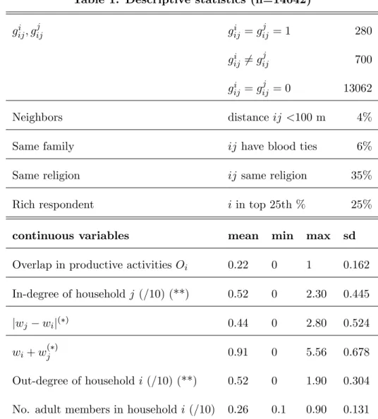
Descriptive statistics are reported Table 1. The …rst and second panels of the table present dichotomous and continuous variables, respectively. In the dataset there are 119 households, which make 119*118=14042 dyads in total. We see from the table that the proportion of pairs for which gi

ij or g j

ji = 1 is 7%. The proportion of discordant responses is large. Around one

third of household pairs share the same religion. Wealth and the other continuous regressors display a healthy amount of variation in the data. Some regressors were rescaled to facilitate estimation.13

1 2

Data on land was collected in acres, but transformed in monetary equivalent using a conversion rate of 300000 tzs for 1 acre. This re‡ects the average local price in 2000, the time at which the data were collected.

1 3

Table 1: Descriptive statistics (n=14042)

gi_ij; gj_ij gi_ij = g_ijj = 1 280

gi_{ij 6= gij}j 700

gi_ij = g_ijj = 0 13062

Neighbors distance ij <100 m 4%

Same family ij have blood ties 6%

Same religion ij same religion 35%

Rich respondent i in top 25th % 25%

continuous variables mean min max sd

Overlap in productive activities Oi 0.22 0 1 0.162

In-degree of household j (/10) (**) 0.52 0 2.30 0.445

jwj wij( ) 0.44 0 2.80 0.524

wi+ wj( ) 0.91 0 5.56 0.678

Out-degree of household i (/10) (**) 0.52 0 1.90 0.304 No. adult members in household i (/10) 0.26 0.1 0.90 0.131

(*) 1 unit corresponds to 1 million Tanzanian Shillings. (**) excluding the ij link

4. Empirical results

4.1. Model estimation

We now estimate models (2.3), (2.6) and (2.9). Each model includes the list of Xij regressors

presented in Table 1. For each set of results the z-values reported in the last column are based on dyadic standard errors corrected using formula (2.10).

risk sharing question capture willingness to link, as explained in subsection (2.1). Coe¢ cients estimates are reported in Table 2 using probit. They suggest that respondents prefer to link with popular households who live nearby, are related, and share a similar level of wealth. The coe¢ cient of wi+ wj is positive and marginally signi…cant, suggesting that willingness to link

is higher among wealthy households. Other regressors are not signi…cant.

Table 2: Willingness to link

Regressor coe¢ cient dyadic z

Overlap in activities Oij -0.194 -0.85

Popularity P_ji 0.508 7.71***

Neighbor dummy 0.760 5.17***

Blood ties dummy 0.987 5.86***

Same religion dummy 0.169 1.31

jwj wij -0.250 -2.35**

wi+ wj 0.249 1.74*

Out-degree of i 0.287 1.65*

Rich dummy of i -0.004 -0.04

Nber adult members of i 0.105 0.26

Intercept -2.659 -15.99***

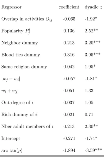
We then turn to the bilateral link formation model (2.6).14 _{Results are presented in Table}

3. Several coe¢ cient estimates are similar to those reported in Table 2. Popularity P_ji remains

strongly signi…cant. Coe¢ cient estimates are again suggestive of homophyly. Overlap in

activi-1 4_{We also estimated the model with alternative assumptions about misreporting, e.g., assuming that discordant}

pairs are due to over-reporting only (i.e., gij = giijgjji) or under-reporting only (i.e., gij = 1 whenever g i ij or

gj_ji= 1). These versions yield parameter estimates that are by and large comparable to those reported in Table 3. But the Vuong test cannot be used to compare these alternative versions to the willingness to link model (2.3) because they use di¤erent dependent variables.

ties Oij is now marginally signi…cant with the anticipated sign, suggesting a desire to link with

individuals who have a di¤erent income pro…le.

Table 3: Bilateral link formation

Regressor coe¢ cient dyadic z

Overlap in activities Oij -0.065 -1.92*

Popularity P_ji 0.136 2.52**

Neighbor dummy 0.213 3.20***

Blood ties dummy 0.316 3.95***

Same religion dummy 0.042 1.95*

jwj wij -0.057 -1.81*

wi+ wj 0.051 1.33

Out-degree of i 0.037 1.05

Rich dummy of i 0.021 0.71

Nber adult members of i 0.213 2.30**

Intercept -0.271 -1.74*

arc tan( ) -1.894 -3.59***

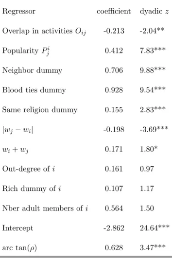
Next we present the results assuming that the data were generated by the unilateral link formation model (2.9). As explained in subsection (2.3), we transform household responses g_iji

and gj_ij into the equation-level dependent variables hi_ij 1 g_iji and hj_ij 1 g_ijj. Results are

reported in Table 4. To facilitate comparison with Table 3, we report estimated coe¢ cients b di-rectly, which means inverting the sign of the coe¢ cient estimates obtained from estimating (2.9) with partial observability bivariate probit. In terms of coe¢ cient estimates, results are similar to those reported in Table 3. Popularity P_ji and activity overlap Oij are both signi…cant with

are not.

Table 4: Unilateral link formation

Regressor coe¢ cient dyadic z

Overlap in activities Oij -0.213 -2.04**

Popularity P_ji 0.412 7.83***

Neighbor dummy 0.706 9.88***

Blood ties dummy 0.928 9.54***

Same religion dummy 0.155 2.83***

jwj wij -0.198 -3.69***

wi+ wj 0.171 1.80*

Out-degree of i 0.161 0.97

Rich dummy of i 0.107 1.17

Nber adult members of i 0.564 1.50

Intercept -2.862 24.64***

arc tan( ) 0.628 3.47***

4.2. Speci…cation tests

We now turn to the main object of the paper, which is to compare the performance of the di¤erent models in accounting for the data. As explained in Section 2, we proceed by pairwise comparisons, adapting the non-nested Vuong test to the dyadic structure of the data. To compare two models k and m we calculate, for each observation ij, the log-likelihood contributions (or score) under the two models and we regress the di¤erence l_ijk l_ijm on a constant, correcting the

standard errors using formula (2.10). The t-value of the constant is the Vuong test corrected for dyadic non-independence. Since the distribution of the Vuong test is asymptotically normal, the relevant critical value for a 5% level of signi…cance is 1:96. Note that the test works in two

directions: if t > 1:96 model k is to be preferred to model m; if t < 1:96 model m is to be preferred to model k. For values of t between 1:96 and 1:96 the test is inconclusive – both models …t the data equally.

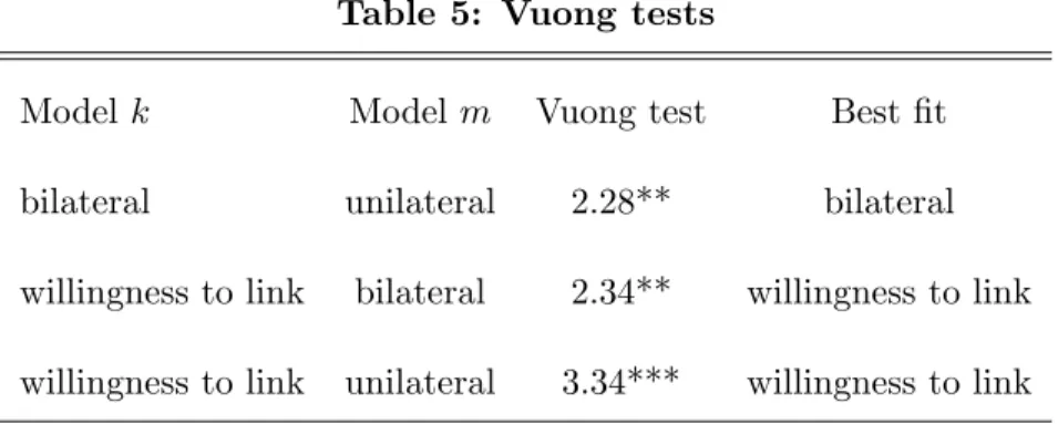
Table 5 reports the result of the pairwise comparisons between the willingness-to-link model and the other two. When the bilateral and unilateral models are compared to each other, the bilateral model is found superior. But the Table unambiguously shows that the willingness-to-link model …ts the data best.

Table 5: Vuong tests

Model k Model m Vuong test Best …t

bilateral unilateral 2.28** bilateral

willingness to link bilateral 2.34** willingness to link willingness to link unilateral 3.34*** willingness to link

4.3. Self-censoring

Our results imply that responses given to the mutual insurance question are best understood as indicative of willingness to link than evidence of an actual link. Yet De Weerdt and Fafchamps (2007) have shown that gi_ij is a strong predictor of gifts and transfers reported in subsequent

survey rounds. Fafchamps and Gubert (2007) report similar …ndings with data collected in the Philippines using a similarly worded question.15 Responses to the mutual insurance question

may be more than just willingness to link.

In particular, we suspect that respondents did not report households with whom they would like to share risk but who are likely to turn them down. Self-censoring has been discussed in the economic literature on dating. In that literature, the researcher typically has access to information on willingness to date – e.g., answers to a direct question following speed dating

interviews (e.g. Belot and Francesconi n.d., Fisman et al. 2008), or emails sent to prospective partners on an internet dating site (Hitsch et al. 2005). In both cases, the authors worry that respondents may fail to list or contact desirable partners who are unlikely to accept them.16

A similar kind of self-censoring may also be at work in our data. In particular, household i may have liked to share risk with household j but expected j to refuse, and so failed to mention j as possible mutual insurance link. This corresponds to an alternative data generating process in which j can veto a link that i wants.

Such data generating process can be represented as follows. As before, g_iji is i’s report of

whether a link to j exists. This report is now thought of as made of two parts: (1) i’s willingness to link with j, which we denote wij; and (2) i’s expectation of whether the link would be accepted

by j, which we denote eij. Expectation eij is thought of as made of two intermingled parts: j’s

willingness to link with i and j’s inability to refuse a link with i even though j does not want to link with i. We observe gi

ij = 1 if both wij = 1 and eij = 1. We observe giji = 0 if either wij = 0

or eij = 0 or both.

To illustrate what we have in mind, imagine that unpopular households wish to link to pop-ular households (wij = 1) but popular households never wish to link with unpopular households

(wji = 0). Yet popular households cannot refuse to help some of the unpopular ones, e.g.,

members of their church. In that case, unpopular household i will report gi_ij = 1 with popular

household j whenever i expects that j will not refuse to help (eij = 1) because of social norms

or altruism. Formally we have:

Pr(g_iji = 1) = Pr(wij = 1 and eij = 1) (4.1)

1 6_{Self-censoring has also been discussed in the context of matching models in which individuals can only rank}

a subset of their possible choices (e.g., schools or jobs). In such models, it is optimal for low ranked individuals not to ‘waste’limited slots on options they are unlikely to get.

with

Pr(wij = 1) = xij

Pr(eij = 1) = xji

Model (4.1) can be estimated using bivariate probit with partial observability. The only di¤erence with model (2.5) is that we no longer impose that coe¢ cients be the same in the two equations. Instead, we now estimate di¤erent coe¢ cients and for the two equations. As before, the estimator allows for non-independence between Pr(wij = 1) and Pr(eij = 1) (for

instance because of unobserved individual e¤ects common to both). Model (4.1), which we call the ‘vetoed link’model, can be seen as a re…ned version of willingness to link which incorporates expectations about the potential partner’s likely behavior.

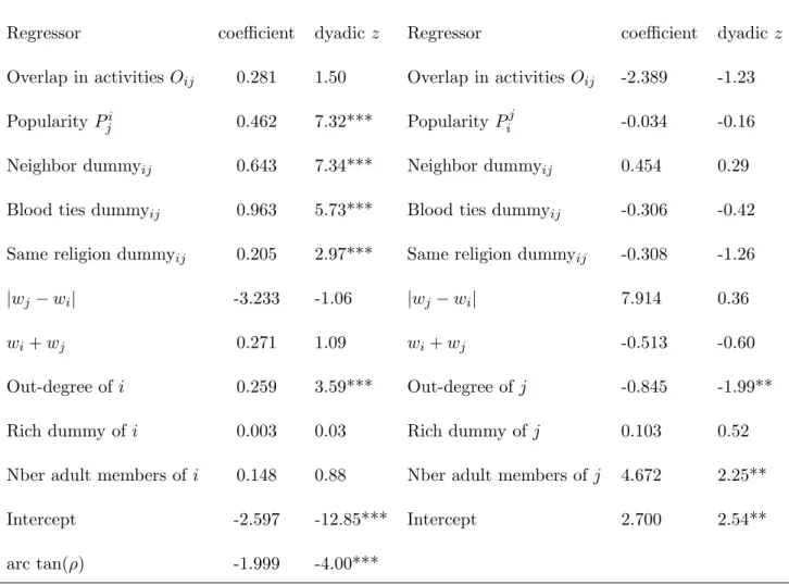
Estimation results for the vetoed link model are presented in Table 6. Coe¢ cient estimates for the wij equation have the same interpretation as before. Coe¢ cient estimates for the eij

equation capture two kinds of e¤ects: j’s willingness to link with i, and j’s capacity to veto a link with i. Bilateral link formation model (2.6) is a restricted form of (4.1) with = , which is equivalent to assuming that i’s statement about the existence of a link with j only depends on j’s willingness to link. Put di¤erently, in model (2.6), i’s statement regarding a link with j internalizes both i’s and j’s willingness to link. The symmetry of (2.6) is equivalent to setting = and implies that g_iji and g_jij have the same probability, i.e., both i and j are equally

likely to report link gij. Model (4.1) allows giji and g j

ji to have di¤ering probabilities depending

on the characteristics of i and j. The willingness to link model (2.3) corresponds to the case where = 0: i’s answer only depends on i’s desire to link with j. Model (4.1) sits between both extremes in that it allows gi

ij and g j

takes into account more than just own willingness to link. In model (4.1), if < 0 for a given regressor xji, this implies that xji is associated with a lower eij and thus a higher likelihood of

‘veto’ by j. A > 0 in contrast implies that the corresponding xji makes it harder for j to

refuse to assist i.

We see that estimated coe¢ cients in the wij equation are somewhat similar in terms of

magnitude and statistical signi…cance to those reported in earlier regressions: popularity P_iji is

again strongly signi…cant, and so are geographical proximity and a shared religion. The out-degree of i (omitting the ij link) is also statistically signi…cant. In contrast, coe¢ cients in the eij regression are quite di¤erent from those reported for the wij equation. Only three coe¢ cients

are statistically signi…cant: the kinship dummy, j’s out-degree, and the size of j’s household. This means that kin are less likely to veto a link but the smaller j’s household is and the larger j’s out-degree, the more likely j will veto a link with i. This suggests that larger households have a duty to care for others, possibly because their size makes them better able to self-insure –and thus to assist others.

Table 6. Vetoed links model

wij equation eji equation

Regressor coe¢ cient dyadic z Regressor coe¢ cient dyadic z

Overlap in activities Oij 0.281 1.50 Overlap in activities Oij -2.389 -1.23

Popularity P_ji 0.462 7.32*** Popularity P_ij -0.034 -0.16

Neighbor dummyij 0.643 7.34*** Neighbor dummyij 0.454 0.29

Blood ties dummyij 0.963 5.73*** Blood ties dummyij -0.306 -0.42

Same religion dummyij 0.205 2.97*** Same religion dummyij -0.308 -1.26

jwj wij -3.233 -1.06 jwj wij 7.914 0.36

wi+ wj 0.271 1.09 wi+ wj -0.513 -0.60

Out-degree of i 0.259 3.59*** Out-degree of j -0.845 -1.99**

Rich dummy of i 0.003 0.03 Rich dummy of j 0.103 0.52

Nber adult members of i 0.148 0.88 Nber adult members of j 4.672 2.25**

Intercept -2.597 -12.85*** Intercept 2.700 2.54**

arc tan( ) -1.999 -4.00***

By analogy with Section 2, it is also possible to de…ne the ‘dual’analogue of the vetoed link model. In this model, i reports his unwillingness to link with j, except in cases when j can impose a link with i. This implies that i reports gi_ij = 1 whenever i expects j to impose a link

on i, even if i is not keen to link with j. In this model, we have:

with

Pr(wij = 0) = xij

Pr(eij = 0) = xji

This model is the generalized equivalent of the unilateral link formation with hij = 1 gij.

It can be estimated in a fashion similar to (4.1), but the interpretation is slightly di¤erent. Here i reports a missing link (g_iji = 0) if i does not want to link and i expects that j cannot impose

a link on i. But i reports a link whenever either i wishes to link with j or i expects that j can impose a link. We call this model the ‘forced link’model since j can force a link that i does not want.

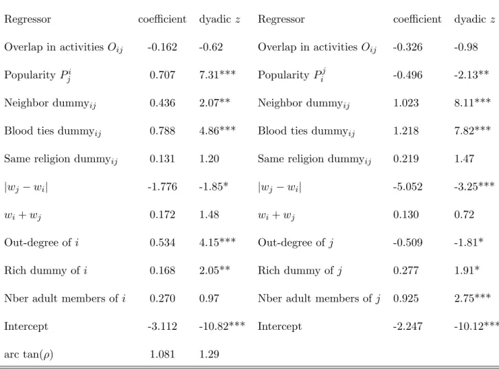
Regression estimates are shown in Table 7. As we did for Table 4, we report estimated coe¢ cients b and _{b directly, i.e., we invert their sign to facilitate comparison with Table 6.} Interpretation of the coe¢ cients of the wij equation is as before. In the case of the eij equation,

= means that i expect j to force a link with i based purely on his/her willingness to link with i. This would arise for instance if i fully internalizes the unilateral link formation equilibrium. In contrast, if all = 0, g_iji is consistent with pure willingness to link. A > 0 means that the

xji variable raises the likelihood that, in i’s opinion, j’s can force a link on i.

Coe¢ cient estimates for the wij equation are fairly similar to those reported earlier in Table

2, except that wi + wj is not marginally signi…cant anymore and i’s out-degree and i’s rich

dummy are now statistically signi…cant. Coe¢ cient estimates for the eij equation are di¤erent

in sign and magnitude from those of the wij equation, a result that is consistent with our earlier

…nding that gi_ij is not consistent with a unilateral link formation process. Several regressors have

that j be willing and able to force a link onto i. Geographical proximity and blood ties appear with a strongly signi…cant positive coe¢ cient, indicating that it is di¢ cult to deny assistance to kin and neighbors. The negative coe¢ cient for i’s popularity P_ij indicates that the more popular

i is, the less likely it is that j can impose a link onto i.

Table 7. Forced links model

wij equation eji equation

Regressor coe¢ cient dyadic z Regressor coe¢ cient dyadic z

Overlap in activities Oij -0.162 -0.62 Overlap in activities Oij -0.326 -0.98

Popularity P_ji 0.707 7.31*** Popularity P_ij -0.496 -2.13**

Neighbor dummyij 0.436 2.07** Neighbor dummyij 1.023 8.11***

Blood ties dummyij 0.788 4.86*** Blood ties dummyij 1.218 7.82***

Same religion dummyij 0.131 1.20 Same religion dummyij 0.219 1.47

jwj wij -1.776 -1.85* jwj wij -5.052 -3.25***

wi+ wj 0.172 1.48 wi+ wj 0.130 0.72

Out-degree of i 0.534 4.15*** Out-degree of j -0.509 -1.81*

Rich dummy of i 0.168 2.05** Rich dummy of j 0.277 1.91*

Nber adult members of i 0.270 0.97 Nber adult members of j 0.925 2.75***

Intercept -3.112 -10.82*** Intercept -2.247 -10.12***

arc tan( ) 1.081 1.29

While these results are interesting in their own right, our primary interest is to test whether either of these models …ts the gi_ij data better than the pure willingness to link model. The

that both signi…cantly dominate the willingness to link model.17 This is consistent with the

idea that reported links g_iji are best interpreted as self-censored willingness to link. The last

row of the Table also shows that we cannot distinguish between the vetoed link and forced link model: although the vetoed link provides a slightly better …t, the di¤erence is not statistically signi…cant. This is not entirely surprising given that the two models are fairly similar in terms of the underlying data generation process.

Table 8: Vuong test –vetoed links and forced links

model k model m Vuong test best …t

vetoed links willingness to link 3.47*** vetoed links

vetoed links bilateral 3.58*** vetoed links

vetoed links unilateral 4.05*** vetoed links

forced links willingness to link 2.65** forced links

forced links bilateral 3.27*** forced links

forced links unilateral 3.94*** forced links

vetoed links forced links 0.70 both

5. Robustness analysis

To ascertain whether our …ndings are sensitive to the choice of regressors, we reestimate all models using di¤erent sets of explanatory variables. Results, not shown here to save space, indicate that when the included regressors have little predictive power –e.g., when the number of regressors is small –the comparison between models tends to be less conclusive. This is hardly

1 7_{For comparison purposes, we also computed a standard likelihood ratio test to compare the vetoed link and}

bilateral link formation models since the latter is nested in/is a restricted form of the former. The value of the test is 87, which is well above the 1% critical value of 20.1 for a 2_{distribution with 8 degrees of freedom. This con…rms}

that the vetoed link regression dominates the bilateral link formation model. A similar comparison between the forced link and the unilateral link formation model yields a test statistic of 124, which clearly shows that the forced link model dominates. Neither of these test statistics corrects for dyadic correlation across observations, however.

surprising as the problem is common to all non-nested tests. The models are compared in terms of their ability to account for the data. When regressors have little predictive power, all models do rather poorly in predicting observed gi_ij and hence cannot be distinguished.

In most cases, eliminating one or more regressors leaves the models’ranking unchanged but turns some pairwise comparison inconclusive. Dropping some regressors can nevertheless change the models’ranking. In particular, if we drop the in-degree P_ji of j and/or the out-degree of i,

non-nested comparisons indicate that willingness to link ranks lower than bilateral or unilateral link formation. Both self-censored models continue to dominate, however.

Finally, it worth mentioning that we have encountered the convergence di¢ culties that partial observability models are known for. Using a stepping algorithms for non-concave regions of the likelihood function alleviates part of the problem, but occasionally convergence may not be achieved. Also, in our experience the partial observability bivariate probit model is particularly sensitive to the choice of ad-hoc initial values and to multicollinearity, which in some extreme cases may result in the impossibility of computing standard errors.

6. Conclusion

The theoretical literature on networks has shown that the nature of the link formation process – e.g., whether unilateral or bilateral –has a strong e¤ect on the resulting network architecture. In this paper we develop a methodology to test whether network data re‡ect a simple willingness to link or an existing link and, in the latter case, whether this link is generated by an unilateral or bilateral link formation process. Taking the equilibrium concept of pairwise stability as starting point, we propose a methodology to compare bilateral and unilateral processes. Central to this methodology is the observation that unilateral link formation requires that both nodes wish not to form a link for the link not to exist. This formal similarity between the bilateral and

unilateral link formation processes allows us to model them both as partial observability models and to compare them with the appropriate non-nested likelihood test.

We illustrate this methodology with data on informal risk-sharing networks in a Tanzanian village. The data is particularly well suited for our purpose because it covers all households in the community, and because the respondents are asked to enumerate all their network partners. The information provided by respondents is nevertheless open to several interpretations.

One possible interpretation is that responses capture an actual link. This interpretation is consistent with the observation made by De Weerdt and Fafchamps (2007) and Fafchamps and Lund (2003) who have shown that risk sharing links reported by survey respondents strongly predict subsequent inter-household transfers. It however remains unclear what process generates these links. The development literature is uncertain as to whether risk sharing networks should be seen as entirely voluntary, or whether social norms impose an element of moral or social pressure making it di¢ cult for households to refuse helping others. If risk sharing is voluntary, link formation can be modelled as bilateral; if risk sharing is imposed by social norms, unilateral link formation is a more appropriate representation of the data generating process. Using a Vuong non-nested test, we …nd that the bilateral link formation model …ts the data better than a unilateral one.

Another possible interpretation is that responses to a question about mutual insurance links capture the respondent’s willingness to link, not an actual link. This may explain the large proportion of discordant answers whereby i reports a link with j although j does not report a link with i. We test a willingness-to-link model against the bilateral and unilateral link formation models and …nd that willingness to link …ts the data best. This …nding, however, is reversed if we drop the in-degree of j or the out-degree of i as regressors.

investigate two forms of self-censoring. In the …rst one, which we call the vetoed link model, we allow respondents to form expectations about the other party’s ability to refuse a link. In the second, which we call the forced link model, respondents anticipate that they may be unable to refuse certain links. We …nd that both models dominate the other three models, suggesting that self-censoring is present. But we are unable to distinguish between the vetoed and forced link models –both …t the data equally well.

While promising, the approach presented here su¤ers from a number of shortcomings. Test results are ultimately predicated on the assumption that the regressors used in the estimation are reasonable predictors of willingness to link. In the case of the self-censoring models, identi…cation rests on exclusion restrictions that cannot be tested without additional data. The contribution of this paper should therefore be seen as primarily methodological. Stronger inference could be achieved if, in addition to information about links, the survey contained more direct evidence on respondents’willingness to link (or de-link) with other households. Should such data become available together with objective information on social links, the methodology presented here can yield a stronger test of bilateral versus unilateral link formation.

References

Altonji, J. G., Hayashi, F. and Kotliko¤, L. J. (1992). “Is the Extended Family Altruistically Linked? Direct Tests Using Micro Data.”, Americal Economic Review, 82(5):1177–1198.

Ambec, S. (1998), A Theory of African’s Income-Sharing Norm with Enlarged Families. (mimeo-graph).

Anderson, S. and Baland, J.-M. (2002). “The Economics of Roscas and Intrahousehold Resource Allocation.”, Quarterly Journal of Economics, 117(3):963–95.

Arcand, J.-L. and Fafchamps, M. (2008), Matching in Community-Based Organizations. (mimeo-graph).

Azam, J. P. and Gubert, F. (2006). “Migrants’ Remittances and the Household in Africa: A Review of Evidence.”, Journal of African Economies, 15(Supplement 2):426–62.

Bala, V. and Goyal, S. (2000). “A Non-Cooperative Model of Network Formation.”, Economet-rica, 68(5):1181–1229.

Banerjee, A. V. and Mullainathan, S. (2007), Climbing Out of Poverty: Long Term Decisions under Income Stress. (mimeograph).

Barr, A., Dekker, M. and Fafchamps, M. (2008), Risk Sharing Relations and Enforcement Mech-anisms. (mimeograph).

Barr, A. and Stein, M. (2008), Status and Egalitarianism in Traditional Communities: An Analysis of Funeral Attendance in Six Zimbabwean Villages. (mimeograph).

Belot, M. and Francesconi, M. (n.d.), Can Anyone Be., Technical report.

Bester, C. A., Conley, T. G. and Hansen, C. B. (2008), Inference with Dependent Data Using Cluster Covariance Estimators. (mimeograph).

Binswanger, H. P. and McIntire, J. (1987). “Behavioral and Material Determinants of Production Relations in Land-Abundant Tropical Agriculture.”, Econ. Dev. Cult. Change, 36(1):73–99.

Charness, G. and Jackson, M. O. (2007). “Group Play in Games and the Role of Consent in Network Formation.”, Journal of Economic Theory, 136:417–45.

Coate, S. and Ravallion, M. (1993). “Reciprocity Without Commitment: Characterization and Performance of Informal Insurance Arrangements.”, J. Dev. Econ., 40:1–24.

Comola, M. (2007), The Network Structure of Informal Arrangements: Evidence from Rural Tanzania., Technical report, INRA-LEA Working Paper 708, Paris.

Conley, T. (1999). “GMM Estimation with Cross-Sectional Dependence.”, Journal of Econo-metrics, 92(1):1–45.

De Weerdt, J. and Dercon, S. (2006). “Risk-Sharing Networks and Insurance Against Illness.”, Journal of Development Economics, 81(2):337–56.

De Weerdt, J. and Fafchamps, M. (2007), Social Networks and Insurance against Transitory and Persistent Health Shocks. (mimeograph).

Ellsworth, L. (1989), Mutual Insurance and Non-Market Transactions Among Farmers in Burk-ina Faso, University of Wisconsin. Unpublished Ph.D. thesis.

Fafchamps, M. and Gubert, F. (2007). “The Formation of Risk Sharing Networks xxx.”, Journal of Development Economics, 83(2):326–50.

Fafchamps, M. and Lund, S. (2003). “Risk Sharing Networks in Rural Philippines.”, Journal of Development Economics, 71:261–87.

Fisman, R., Iyengar, S., Kamenica, E. and Simonson, I. (2008). “Racial Preferences in Dating.”, Review of Economic Studies, 75:117–32.

Genicot, G. and Ray, D. (2003). “Group Formation in Risk-Sharing Arrangements.”, Review of Economic Studies, 70(1):87–113.

Goyal, S. (2007), Connections: An Introduction to the Economics of Networks, Princeton Uni-versity Press, Princeton and Oxford.

Granovetter, M. (1985). “Economic Action and Social Structure: The Problem of Embedded-ness.”, Amer. J. Sociology, 91(3):481–510.

Hitsch, G. J., Hortacsu, A. and Ariely, D. (2005), What Makes You Click: An Empirical Analysis of Online Dating, University of Chicago and MIT, Chicago and Cambridge.

Jackson, M. O. (2008), Social and Economic Networks xxx, Princeton University Press, Prince-ton.

Jackson, M. O. and Wolinsky, A. (1996). “A Strategic Model of Social and Economic Networks.”, Journal of Economic Theory, 71(1):44–74.

Kimball, M. S. (1988). “Farmers’Cooperatives as Behavior Toward Risk.”, Amer. Econ. Rev., 78 (1):224–232.

Kocherlakota, N. R. (1996). “Implications of E¢ cient Risk Sharing Without Commitment.”, Rev. Econ. Stud., 63(4):595–609.

Lucas, R. E. and Stark, O. (1985). “Motivations to Remit: Evidence from Botswana.”, J. Polit. Econ., 93 (5):901–918.

Platteau, J.-P. (1995). “An Indian Model of Aristocratic Patronage.”, Oxford Econ. Papers, 47(4):636–662.

Platteau, J.-P. (1996), Traditional Sharing Norms as an Obstacle to Economic Growth in Tribal Societies., Technical report, CRED, Facultés Universitaires Note-Dame de la Paix, Namur, Belgium. Cahiers No. 173.

Poirier, D. (1980). “Partial Observability in Bivariate Probit Models.”, Journal of Econometrics, 12:209–17.

Scott, J. C. (1976), The Moral Economy of Peasant: Rebellion and Subsistence in South-East Asia, Yale University Press, New Haven.

Townsend, R. M. (1994). “Risk and Insurance in Village India.”, Econometrica, 62(3):539–591.

Vandenbossche, J. and Demuynck, T. (2009), Network Formation with Absolute Friction and Heterogeneous Agents. (mimeograph).

Vega-Redondo, F. (2006), Complex Social Networks xxx, Cambridge University Press, Cam-bridge.

Vuong, Q. H. (1989). “Likelihood Ratio Tests for Model Selection and Non-Nested Hypotheses.”, Econometrica, 57, No. 2:307–333.