HAL Id: hal-00317496
https://hal.archives-ouvertes.fr/hal-00317496
Submitted on 31 Jan 2005
HAL is a multi-disciplinary open access
archive for the deposit and dissemination of
sci-entific research documents, whether they are
pub-lished or not. The documents may come from
teaching and research institutions in France or
abroad, or from public or private research centers.
L’archive ouverte pluridisciplinaire HAL, est
destinée au dépôt et à la diffusion de documents
scientifiques de niveau recherche, publiés ou non,
émanant des établissements d’enseignement et de
recherche français ou étrangers, des laboratoires
publics ou privés.
IMAGE FUV and EISCAT measurements
N. Østgaard, J. Moen, S. B. Mende, H. U. Frey, T. J. Immel, P. Gallop, K.
Oksavik, M. Fujimoto
To cite this version:
N. Østgaard, J. Moen, S. B. Mende, H. U. Frey, T. J. Immel, et al.. Estimates of magnetotail
reconnection rate based on IMAGE FUV and EISCAT measurements. Annales Geophysicae, European
Geosciences Union, 2005, 23 (1), pp.123-134. �hal-00317496�
SRef-ID: 1432-0576/ag/2005-23-123 © European Geosciences Union 2005
Annales
Geophysicae
Estimates of magnetotail reconnection rate based on IMAGE FUV
and EISCAT measurements
N. Østgaard1, J. Moen2,3, S. B. Mende1, H. U. Frey1, T. J. Immel1, P. Gallop4, K. Oksavik2, and M. Fujimoto5
1Space Sciences Laboratory, University of California, Berkeley, California, USA
2Department of Physics, University of Oslo, Norway
3University Centre on Svalbard, Longyearbyen, Norway
4Rutherford Appleton Laboratory, Oxfordshire, UK
5Department of Earth and Planetary Sciences, Tokyo Institute of Technology, Japan
Received: 16 September 2003 – Revised: 15 March 2004 – Accepted: 30 March 2004 – Published: 31 January 2005 Part of Special Issue “Eleventh International EISCAT Workshop”
Abstract. Dayside merging between the interplanetary and
terrestrial magnetic fields couples the solar wind electric field to the Earth’s magnetosphere, increases the magnetospheric convection and results in efficient transport of solar wind en-ergy into the magnetosphere. Subsequent reconnection of the lobe magnetic field in the magnetotail transports energy into the closed magnetic field region. Combining global imag-ing and ground-based radar measurements, we estimate the reconnection rate in the magnetotail during two days of an EISCAT campaign in November-December 2000. Global images from the IMAGE FUV system guide us to identify ionospheric signatures of the open-closed field line bound-ary observed by the two EISCAT radars in Tromsø (VHF) and on Svalbard (ESR). Continuous radar and optical mon-itoring of the open-closed field line boundary is used to de-termine the location, orientation and velocity of the open-closed boundary and the ion flow velocity perpendicular to this boundary. The magnetotail reconnection electric field is found to be a bursty process that oscillates between 0 mV/m and 1 mV/m with ∼10–15 min periods. These ULF oscilla-tions are mainly due to the motion of the open-closed bound-ary. In situ measurements earthward of the reconnection site in the magnetotail by Geotail show similar oscillations in the duskward electric field. We also find that bursts of increased magnetotail reconnection do not necessarily have any asso-ciated auroral signatures. Finally, we find that the reconnec-tion rate correlates poorly with the solar wind electric field. This indicates that the magnetotail reconnection is not di-rectly driven, but is an internal magnetospheric process. Es-timates of a coupling efficiency between the solar wind elec-tric field and magnetotail reconnection only seem to be rel-evant as averages over long time intervals. The oscillation mode at 1 mHz corresponds to the internal cavity mode with
Correspondence to: N. Østgaard
additional lower frequencies, 0.5 and 0.8 mHz, that might be modulated by solar wind pressure variations.
Key words. Magnetospheric physics (magnetotail; electric
fields; magnetosphere ionosphere interaction; solar wind -magnetosphere interaction). Space plasma physics (magnetic reconnection)
1 Introduction
A fundamental element of the open magnetosphere model first suggested by Dungey (1961) is that dayside merging and subsequent magnetotail reconnection transfer solar wind plasma and energy to the magnetospheric-ionospheric sys-tem. Dayside reconnection generates open magnetic flux whereas the magnetotail cross-tail reconnection destroys open flux by converting it back to closed flux. The cycle of accumulation and loss of open flux is also related to the mag-netospheric behavior during substorms. In the Dungey cycle this circulation of flux was assumed to be a steady-state phe-nomenon, with the rates of merging on the dayside and re-connection in the tail balancing each other. However, as sug-gested by Russell (1972), the two processes may be viewed as two separate time-dependent processes. This means that while dayside merging is thought to be controlled by the in-terplanetary magnetic field (IMF), magnetotail reconnection may not have a similar strong IMF dependence.
Reconnection may occur at two different locations in the magnetotail. The first type of reconnection is associated with the formation of the far X-line and defines the last closed field line of the magnetosphere. A second type, which is more controversial, is associated with the formation of the near Earth neutral line (NENL). We do not know if this type of reconnection is controlled by the solar wind, IMF, or is entirely controlled by some internal magnetospheric
instabil-ities or some combination thereof. However, if the reconnec-tion rate at the NENL locareconnec-tion exceeds that at the far X-line location, the open-closed boundary will approach the NENL and its ionospheric footpoint will move equatorward. At this moment the last closed field line will thread both the NENL and the far X-line. The newly formed NENL will then be-come the new far X-line, which will propagate tailward. This tailward motion is associated with a poleward motion of the open-closed boundary in the ionosphere.
As the far X-line or the NENL defines the boundary be-tween open-closed field lines it has been shown theoretically that the plasma flow through the open-closed boundary in the ionosphere can be utilized to estimate the reconnection elec-tric field in the magnetotail (Vasyliunas, 1984).
Crucial for this method is, however, how accurate one is able to determine the open-closed boundary. According to Lockwood (1997) the open-closed boundary can be identi-fied from the diffuse electron precipitation from the plasma sheet boundary layer or from the equatorward drifting arcs which form just equatorward of the open-closed boundary (Fujii et al., 1994; Hoffman et al., 1994) and are embedded in this diffuse precipitation. These arcs are also associated with intense electric fields (Pedersen et al., 1985) and thought to be Alfv´en wave signatures of processes near or at the re-connection line (Hesse et al., 1999; Yamade et al., 2000). The accuracy by which one can determine the open-closed boundary is therefore highly dependent on the sensitivity and spatial resolution of the instruments that are used. Lockwood (1997) suggested that the open-closed boundary is roughly 200 km poleward of where an imager from space will place the open-closed boundary.
A few studies have reported quantitative results of the re-connection electric field in the magnetotail and have used dif-ferent ways to identify the open-closed boundary.
de la Beaujardi´ere et al. (1991) used incoherent scatter radar data from Søndre Strømfjord to obtain the plasma flow and to locate the open-closed boundary. The latter was de-termined from gradients of the density in the ionospheric E-region layer as precipitating energetic electrons enhance the density in the auroral oval relative to the polar cap. They reported ionospheric projections of the reconnection electric field to be 20–40 mV/m.
A similar method was used by Blanchard et al. (1996, 1997). In addition to the gradient of E-region electron
den-sity they used the 6300 ˚A emissions from an all-sky camera
to define the open-closed boundary. They found the iono-spheric projection of the reconnection electric field to vary between 0–60 mV/m. Compared to the solar wind electric field they found an average coupling efficiency of 0.1 and a maximum correlation when introducing a 70-min timelag to the solar wind data. They also found that the reconnec-tion rate increased significantly during the expansion phase of substorms.
Ober et al. (2001) used in-situ measurements to estimate the reconnection electric field just as the Polar satellite tra-versed the open-closed boundary during the expansion phase of a substorm. Combined particle, electric field and
mag-netic field measurements were used to determine the ion flow perpendicular to the open-closed boundary, and images from the VIS Earth camera (130.4 nm) were used to determine the boundary velocity. Although no temporal information can be extracted from such a boundary crossing, their result repre-sents an important in-situ measurement of the reconnection electric field. They found the ionospheric projection of the reconnection electric field to be 20–70 mV/m.
In this paper we have used images from IMAGE FUV and data from the EISCAT VHF radar in Tromsø (VHF) and the EISCAT Svalbard radar (ESR) to estimate the reconnection rate during two time intervals of an EISCAT campaign in November-December 2000. On 28 November 2000, the ex-pansion and recovery phase of a relatively strong substorm was observed by IMAGE and the Tromsø VHF radar. The data from 7 December 2000 were obtained during a quieter geomagnetic time, although a clear auroral intensification, which may be classified as a weak substorm, was observed by IMAGE and the EISCAT Svalbard radar. Section 2 de-scribes the instruments and data quality, Section 3 gives an overview of the theoretical framework developed by Vasyli-unas (1984) as well as the geometry of the observations. The events are presented in Sections 4 and 5, while the discussion and conclusions are presented in Sections 6 and 7.
2 Instrumentation and data processing
The IMAGE FUV instrumentation consists of two different cameras, the wide band imaging camera (WIC) and the spec-trographic imager (SI). The SI provides separate measure-ments of the O line at 135.6 nm (SI13) and the Doppler-shifted Lyman α emission at 121.8 nm (SI12), the latter de-signed to measure auroral emissions from proton precipita-tion. For boundary determination and auroral intensity we use measurements from the WIC camera, as this camera has the highest sensitivity and spatial resolution. The WIC camera measures FUV emissions in the 140–180 nm
wave-length range. These are N2emissions in the
Lyman-Birge-Hopfield band and a few N emission lines. These emissions are all prompt emissions which result in highly detailed au-roral images. The sensitivity of the WIC camera, mean-ing the auroral intensity needed for the aurora to be distin-guished from noise, after background subtraction, is about 100 counts/pixel or ∼250 R. The spatial resolution depends on the altitude of the spacecraft, but is ∼100 km at apogee (8
RE geocentric distance). For a more complete description of
the FUV imaging system, see Mende et al. (2000) and Frey et al. (2003).
The two incoherent-scatter radars in Tromsø (VHF) and on Svalbard (ESR) provide measurements of the electron den-sity, electron and ion temperature and the ion flow velocity along the radar beam. This study uses the electron tempera-ture for open-closed boundary determination and the ion flow velocity across this boundary to estimate the reconnection electric field.
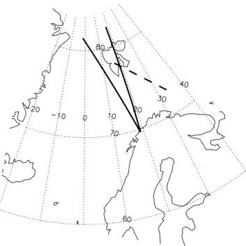
Figure 1 shows the radar beam directions for the two days of observations, when mapped down along the magnetic field to 100 km altitude. One of the VHF beams (Tromsø) was directed approximately along the magnetic meridian (west beam), while the other beam was directed towards geo-graphic north (north beam). The radar sampled data in 19 range intervals at altitudes from 230 km to 1052 km and the integration time used in the data analysis is 1 minute. As ex-plained in Section 3.1, only data sampled above 300 km are used, which corresponds to intervals 5–19. The spatial reso-lution in the beam direction, when mapped down to 100 km altitude, ranges from ∼30 km (interval 5) to ∼140 km
(in-terval 19). The EISCAT Svalbard radar was directed at 135◦
azimuth from geographic north with a 30◦elevation and
sam-pled data at altitudes from 106 km to 596 km. These data are analyzed with a 26 s integration time in 16 spatial inter-vals, where only data above gate 9 (>300 km) can be used. The spatial resolution for the latter (at 100 km) ranges from
∼30 km (gate 9) to ∼60 km.
3 Approach
3.1 Method to calculate the reconnection rate
The method to calculate the reconnection electric field from the ion flow across the open-closed boundary in the night-side ionosphere is based on the theoretical approach pre-sented by Vasyliunas (1984). As sketched in Fig. 2 the
X-line in the magnetotail, Cm, is connected to the ionosphere
along the two magnetic field lines, Cp, to form a closed loop
(Cm+Cp+Ci+Cp) along the separatrix, which delineates
the area, A. If u is defined as the velocity of the loop, Fara-day’s law (integral form) applied on this closed loop gives us I (E + u × B) · dl = −d dt Z B · dA. (1)
By definition no magnetic field lines cross the separatrix (i.e. the field lines defining the surface of area A) and Eq. (1) can be written Z Cm (E + u × B) · dl + Z rest (E + u × B) · dl = 0, (2)
where rest =Cp+Ci+Cp. In the first term (u × B) · dl=0
because B is either zero or aligned with Cm. For the rest of
the loop the MHD approximation
E + v × B ≈ 0 (3)
can be applied as long as the dimension of the loop is large compared to a characteristic microscopic scale length of the plasma (e.g. a gyroradius) (Vasyliunas, 1984). This approxi-mation applies for a collisionless plasma and holds even for
the segment, Ci, as long as it is placed above the region
where ion-neutral collisions are significant. Using only radar measurements from >300 km, the ratio of gyrofrequency and the ion-neutral collision frequency is well above 100 (Kelley,
Fig. 1. The beam directions, mapped down to 100 km, for the
EIS-CAT VHF radar in Tromsø (solid lines) on 28 November 2000 and for the EISCAT Svalbard radar (dashed line) on 7 December 2000 shown in geographic coordinates.
c
pcc
ppc
mccc
iiv-u
A
Fig. 2. The geometry for estimating the reconnection rate from ion
flow across the open-closed boundary in the nightside ionosphere.
1989, pg. 39). The approximation (Eq. (3) also holds for the
two segments Cp under one of the following assumptions:
The loop is chosen narrow enough so any Ek is the same
on both segments Cp and cancel in the integration.
Alter-nately, Ek≈0, which is probably a reasonable assumption on
the open-closed boundary. Consequently, the MHD approx-imation should hold for the entire loop. Equation (2) can therefore be written as Z Cm E · dl ≈ Z rest ([v − u] × B) · dl (4)
and because the right term is zero along the two field line
segments, Cp, we finally obtain
Z Cm E · dl ≈ Z Ci ([v − u] · B) · dl, (5)
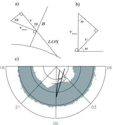
n w n n a) c) b) v v max LOS B v v max α α
Fig. 3. The angles to consider when estimating the ion flow
perpen-dicular to the magnetic field and the open-closed boundary. (a) α is the angle between the magnetic field line and the measured line-of-sight flow velocity. (b) n is the angle between the open-closed boundary and the north beam of the EISCAT VHF radar. (c) All counts above the noise threshold of FUV WIC (21:59:57 UT) are shown in grey. The straight solid lines show the west and north beam of the EISCAT VHF radar and the curved solid line shows the smooth open-closed boundary along the two line of sights. The angles between the line of sight and the boundary for the west and north beam are denoted w and n, respectively. In a) and b) we have indicated the maximum velocity given this geometry.
where v−u is the ionospheric plasma flow velocity perpen-dicular to the magnetic field in the open-closed boundary reference frame. A positive (equatorward) value of v−u is equivalent to a duskward reconnection electric field in the
magnetotail. If 1li is a small segment of Cithat we measure
in the ionosphere we get
Em·1lm≈ [v − u]i·Bi·1li =Ei ·1li, (6)
where 1li is much smaller than 1lm. Assuming that the
width of the magnetotail is 40 RE, the nightside open-closed
boundary scales as (Blanchard et al., 1996)
1lm 1li = 40 RE π ·cos λ RE = Ei Em , (7)
where λ is the magnetic latitude of the open-closed
bound-ary. At 70◦(75◦, 80◦) magnetic latitude 1lmis ∼40 (∼50,
∼75) times larger than 1li and consequently, Em will be
∼40 (∼50, ∼75) smaller than Ei.
3.2 How to determine the open-closed boundary location
and geometry
In addition to the ion velocity, we need to determine the location, orientation and motion of the open-closed bound-ary. This information can be obtained from the IMAGE/FUV WIC images.
Figure 3c shows the image from 28 November 2000 at 21:59:57 UT. After background subtraction a threshold of 100 counts/pixel (∼250 R) was found to be the lowest count rate where the auroral emissions can be distinguished from noise. Along the direction of the radar beams (solid thick lines) the open-closed boundary can be defined as the pole-ward edge of the aurora, i.e. where the count rates fall be-low 100 counts/pixel (or ∼250 Rayleigh). From the im-ages we can also define the angles between the radar beams and this boundary, denoted w and n, for the west and north beams, respectively (Figs. 3b and c). As the EISCAT data only gives us the ion flow along the beam direction, these angles are needed to calculate the ion flow perpendicular to the boundary. A second angle to consider is the angle be-tween the magnetic field and the beam direction, denoted
αin Fig. 3a. Under the assumption that the ion velocity is
uniform on the scale size that separates the west and north
beam (14.7◦, which corresponds to a maximum separation
less than 350 km), we can combine the ion velocities from the west and north beams to calculate the ion velocity per-pendicular to the boundary more accurately. In this case the maximum velocity perpendicular to both the boundary and the magnetic field is given by
vmax= v
sin α. (8)
If only one beam direction is available the maximum velocity perpendicular to the boundary and the magnetic field is given by
vmax= v
sin α sin n. (9)
For the boundary velocity we assume that the boundary motion is along the magnetic meridian. This assumption is partly supported by images, but may not always be true and
will be discussed. Consequently, if umis the boundary
ve-locity we measure along the line of sight the veve-locity along the magnetic meridian, u (north beam), is given by
u = um sin n. (10)
For the 28 November event, when two beams can be com-bined to calculate the ion velocity perpendicular to the boundary, the maximum ion flow velocity and the boundary velocity given by Eqs. (8 and 10) are used as input in Eq. (6). For the 7 December event, when only measurements along one beam were available, Eqs. (9 and 10) are used as input in Eq. (6).
To take advantage of the better spatial resolution of the radar data, we will use the open-closed boundary determined from the UV images as guidance to confine the location
November 2000 Nov 28, 2000 a) b) c) c)
Fig. 4. The Dst (a) and AE (b) indices prior to and during the
substorm on 28 November 2000. The time interval for the analysis is shown by the grey shaded areas. (c) The substorm development as imaged by the SI13 channel (135.6 nm) of the Spectrographic Imager. Red lines indicate the line of sight of the two beams of the EISCAT VHF radar.
based on the electron temperature measured by the radars. It may be argued that the electron temperature should have been taken from the E-region, where the peak energy de-position associated with diffuse aurora occurs. However, it has been shown theoretically (Kagan et al., 1996) and con-firmed by observations (Doe et al., 1997) that Alfv´en waves and turbulent electrostatic fields can cause significant heat-ing in the F-region associated with downward field-aligned currents closing at the edge of the polar cap. In the absence of such heating one can argue that the F-region heating asso-ciated with precipitation depends on the number flux of pre-cipitating particles, regardless of energy. The number flux of polar rain is usually very low and is easily distinguishable from nightside precipitation on closed field lines. To make sure that we do not misinterpret polar cap F-region heating to be on closed field lines, we will use the electron temperature to define the open-closed boundary when this determination can be confirmed by imaging data. The orientation of the open-closed boundary will be determined from the images.
4 28 November 2000
In Fig. 4a and b we show the geomagnetic conditions prior to and during the event on 28 November. The grey shaded in-terval indicates the time inin-terval when both IMAGE and the EISCAT VHF radar measurements were available (20:00– 22:00 UT). From the provisional Dst index we see that a magnetic storm started late night on 26 November and by
28 November the storm is still in its main phase (Dst at
−60 nT). As expected, the preliminary quick-look AE index
shows rather disturbed conditions (300 nT) even before the substorm occurred. As small parts of the data in some of the WIC images were lost because of a mass memory problem on-board the spacecraft during this time interval, we let a se-quence of SI13 images (Fig. 4(c) display the global auroral activity during this substorm. As the IMAGE spacecraft was coming up from perigee the imagers did not capture the on-set of the substorm, but the poleward, as well as eastward and westward expansion during the substorm expansion phase, is
clearly seen. Figure 5 shows the 1-min VHF data for 28
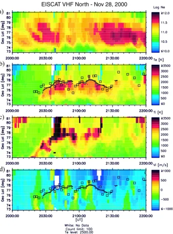
November 2000, 20:00–22:00 UT. A median filter has been applied to the VHF data to remove unreasonable values. The positions of the gates are mapped down to 100 km altitude using the Tsyganenko 2001 model (Tsyganenko, 2002) with the IGRF 2000 and solar wind measurements from Wind as input. The poleward boundaries of the auroral emissions and the electron temperature increase should both be good indi-cators of the open-closed boundary. To take advantage of the better spatial resolution of the radar data, we use the open-closed boundary determined from the images as guidance to confine the location based on the electron temperature mea-sured by the radars. To do this we determine a boundary for 11 different temperatures (1600–2600 K, in 100 K steps) and select the one that correlates best with the boundary de-termined from the images. In Fig. 5b (and d) the bound-ary determined from the images is shown by squares. In this case the boundary determined from an electron temper-ature of 2500 K, shown by a solid thin line, gives the best correlation with the image boundary. The discrepancy be-tween the two boundary determinations is in the range of the
spatial resolution of the WIC images (100 km or ∼1◦). We
should also point out that the very high electron density be-tween 21:30 UT and 22:00 UT will have a cooling effect on the electron temperature and we are not able to identify any boundary from the temperature during this interval. To iden-tify the ion flow velocity we use the value in the gate defining the boundary shown by the thin line (Fig. 5d). We also cal-culate the average of the velocities in the exact gate and in the two gates poleward and equatorward of this. To estimate the velocity of the boundary (u) we use the values shown by the smoothed thick line in order to avoid large steps in veloc-ity due the spatial resolution of the radar measurements. The smoothing is performed by a 5-min (5 data points) boxcar av-eraging, meaning that the average of 5 data points represents the center data point.
In Fig. 6a-c the angles and velocities that go into Eq. (8 and 10) to calculate the maximum ion velocity and the boundary
a)
b)
c)
d)
EISCAT VHF North - Nov 28, 2000
Fig. 5. The measurements along the north beam of the EISCAT
VHF radar. The gate positions are mapped along the magnetic field line down to 100 km altitude. Time resolution is 1 min. The four panels show (a) the electron density, Ne, (b) the electron temper-ature, Te, (c) the ion tempertemper-ature, Ti and (d) the ion velocity, Vi, along the line of sight with positive values to the north. The open closed boundary inferred from the Te measurement is shown by solid lines. The thin line is the actual gate position and the thick line is the same boundary smoothed. The squares show the open-closed boundary inferred from the WIC images.
velocity are shown. The reconnection electric field in the magnetotail and its projection to the ionosphere (Figure 6e and 6d) are then calculated from Eqs. 6 and 7). The magnetic latitude (θ ) dependent dipole field strength (in nT) is used as input in these calculations (Eq. (6).
B(θ ) =32000
√
1 + 3 sin θ . (11)
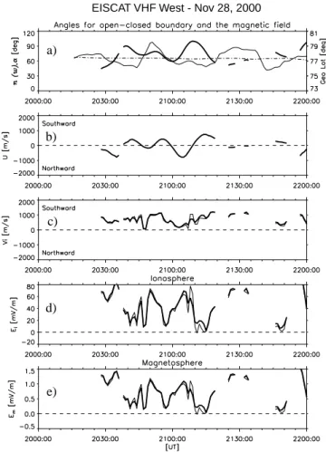
The thin lines in panels (c-e) show the results when the ve-locity in the gate position defining the boundary (thin line in Fig. 5d) is used. The thick lines show the result when the average of this velocity and the velocity in the two gates poleward and equatorward are used. The latter corresponds to the average within 90 km up to a few hundreds of km. As the two lines are nearly on top of each other we feel confident that any uncertainties regarding the boundary determination should not affect our results significantly. The magnetotail reconnection electric field estimated from the north beam is varying between 1.0 mV/m and 0 mV/m. The variations are
EISCAT VHF North - Nov 28, 2000
a)
b)
c)
d)
e)
Fig. 6. The reconnection rate estimated from the north beam: (a)
Thick line: the smoothed geographic latitude of the open-closed boundary, thin line: the angle, n, between the open-closed boundary and the line-of-sight and dashed-dotted line: the angle α, between the magnetic field and the line-of-sight. (b) The smoothed boundary velocity, u Eq. (10) (c) Thin line: the maximum ion flow velocity,
v, Eq. (8) in the gate position defining the open-closed boundary (thin line in Fig. 5d) and thick line: The maximum ion flow velocity when the average of three gate positions are used (d). The iono-spheric projection of the reconnection electric field (Eq. (6) using one v value (thin) and the average of three v-values (thick). (e) The reconnection electric field in the magnetosphere (Eq. (7).
mostly due to ion flow velocity changes, although small os-cillations are seen in the boundary velocity.
In Fig. 7 we show the same parameters estimated from measurements along the west beam. The time and spatial resolution is the same as for the north beam. Along this beam the reconnection rate shows larger variations, which are mostly due to the boundary velocity. We notice that the reconnection rate oscillations have periods of about 15 min.
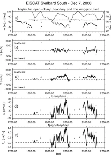
5 7 December 2000
On 7 December 2000 the Svalbard EISCAT radar provided data from 17:00–22:00 UT, while IMAGE provided the global context as well as boundary characteristics along the
radar beam direction. After staying close to 0 nT for 3 h, the AE index (Fig. 8b) increased around 17:00 UT, indicating a small substorm around that time, which was confirmed by images (not shown). The AE index peaked at about 18:20 UT (450 nT), then dropped to about 250 nT and stayed between 250 nT and 300 nT for the rest of the interval. The IMAGE WIC images (Fig. 8c) illustrate the overall activity during the times of radar observations.
The first column (18:00–19:00 UT) shows the substorm that started at 17:00 UT. Around 19:00 UT the aurora stays very quiet for almost two hours until a small break-up, which may be classified as a small substorm, occurred around 20:40 UT.
In Fig. 9 the 26-s EISCAT Svalbard radar data are shown. Regarding open-closed boundary determination, an electron temperature of 1800 K was found to give the best correlation with the boundary determined from the images. For half of the interval (after 19:40 UT) we see that the two data sets give boundary determination within the uncertainties of the
im-age data (100 km or 1◦). During the interval between 18:20–
18:40 UT the images display bright aurora without showing up as any increase in the electron temperature. In the interval from 19:00 UT to 19:40 UT the electron temperature shows
significant increases, giving a clear boundary almost 2◦
pole-ward of the boundary determined from the faint aurora. The angles, velocities and reconnection rate estimated from these measurements are shown in Fig. 10. Again, to avoid large steps in boundary velocity due the spatial res-olution of the radar measurements, we have performed a 2-min (5 data points) boxcar averaging on the boundary and the boundary velocity. In this case, the average ion flow velocity over three intervals (thick line in Fig. 10c) ranges from 90 km to 180 km. Two distinct bursts of increased reconnection rate are seen, one from 19:00–20:00 UT, when the aurora is al-most absent and another from 20:40 UT, when the auroral break-up is seen. The oscillations which are mainly due to the boundary velocity have periods of ∼10 min.
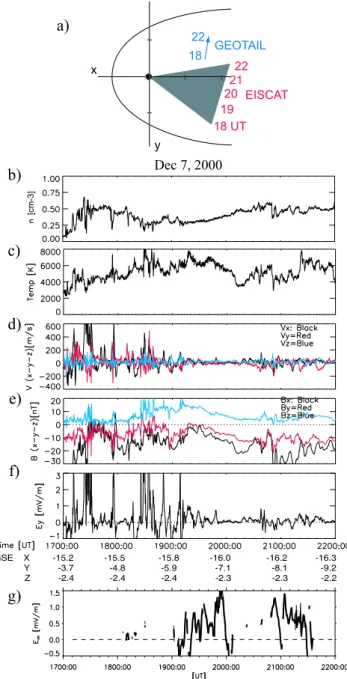
During this event, Geotail measured plasma and magnetic
field parameters in the plasma sheet at X=-15RE2–4 h
dawn-ward of where the EISCAT Svalbard radar measurements were obtained, as illustrated in Fig. 11a. Both the density, temperature and magnetic field measurements indicate that Geotail was in the plasma sheet. Strong bursty bulk flows (BBF) were observed prior to 19:00 UT (Fig. 11d and f), which coincided with auroral activity, but were not associ-ated with any reconnection signatures in the radar data. As such, BBFs are usually observed in a narrow channel in the plasma sheet (Angelopoulos et al., 1992) and the EISCAT Svalbard radar, at this point, might have been measuring on field lines that map to the duskward flank of the magneto-sphere, i.e. outside the region of BBFs. After 19:00 UT Geo-tail moves dawnward, but oscillations on the time scale of 10–15 min can still be seen in the duskward electric field (as
derived from Vxtimes Bzin Fig. 11f) in the interval 19:00–
20:00 UT and around 21:00 UT, with a relatively quiet in-terval in between. Although there is not a one-to-one cor-relation, the oscillations are in the same range (0–1 mV/m)
EISCAT VHF West - Nov 28, 2000
a)
b)
c)
d)
e)
Fig. 7. Same as Fig. 6, but for the west beam.
and on the same time scale as the radar observations reveal (Fig. 11g). This indicates that these oscillations are not lo-calized but extend through large parts of the nightside mag-netosphere.
6 Discussion
The most crucial parameter in our estimate of the magnetotail reconnection electric field is the determination of the open-closed boundary.
Blanchard et al. (1996) used the electron density in the
E-layer (3·1010m−3) combined with latitudinal scans of
630.0 nm emissions and found a rms difference between the
two methods of ±0.6◦.
Ober et al. (2001) used the 130.4 nm images from the Po-lar VIS Earth camera. Due to resonance scattering of this emission it may be argued that the images will be smeared out somewhat and is not so good for determining accurate boundary location.
In this study we have used global imaging data from the IMAGE FUV instruments and the electron temperature from the EISCAT radar measurements to estimate the open-closed boundary. The discrepancies between the two boundary de-terminations are, for most of the time, in the range of the
December 2000 Dec 7, 2000
a)
c)
b)
Fig. 8. (a) Dst and (b) AE indices during the observations on 7 December 2000. (c) IMAGE/ FUV WIC images from 18:00–22:00 UT. The
EISCAT Svalbard radar beam is marked with a red line.
spatial resolution of the images. We have shown that the av-erage of the ion flow velocity in three adjacent spatial inter-vals give the same result as using the ion flow in the exact boundary interval. The spatial averaging applied to the ion velocity ranges from 90–180 km. This means that any error in our boundary determination less than ∼100 km should not affect our result significantly. However, there are some inter-vals when the two techniques give discrepancies larger than the spatial resolution of the images, indicating that the open-closed boundary determination during these times is more uncertain.
Although Blanchard et al. (1996) used all-sky cameras to check the assumption of a boundary orientation parallel to the L-shell at Søndre Strømfjord, they did not have continu-ous information of the boundary orientation as provided by IMAGE FUV during our observations.
In order to calculate the boundary velocity, we have as-sumed that the boundary motion is along the magnetic merid-ian. Although this is partly supported by the images, it may not always be true and represents a source of error in our estimate. This means that variations in the reconnection rate caused by the boundary velocity could sometimes have larger or smaller amplitudes. However, the 5 data-point smoothing
a)
b)
c)
d)
EISCAT Svalbard South - Dec 7, 2000
Fig. 9. Same as Fig. 5, but for the EISCAT Svalbard radar on 7
December 2000. Time resolution is 26 s.
of the boundary location we have performed to avoid large steps in velocity is in fact a way of filtering out large oscilla-tions, which may indicate that we rather underestimate than overestimate these oscillations. To summarize, by properly taking into account the geometry of the observations as well as the uncertainties of our boundary determination, we argue that our estimates should reflect fairly well the real reconnec-tion electric field in the magnetotail.
We find the magnitude of the magnetotail reconnection electric field to be between 0 mV/m and 1 mV/m (or 0– 80 mV/m in the ionospheric projection), which is in good agreement with earlier results (Blanchard et al., 1996; Ober et al., 2001). It is also in the same range as the Geotail in-situ measurements of the electric field earthward of the reconnec-tion site in the magnetotail.
During the observations on 7 December 2000, between 19:00 UT and 20:00 UT, increased reconnection electric field is seen in the ESR data, without showing any significant au-roral intensity increase in the WIC images. However, we do see auroral activity associated with the BBFs observed by Geotail prior to 19:00 UT, consistent with earlier studies (Fairfield et al., 1999; Nakamaura et al., 2001).
Blanchard et al. (1996) estimated a coupling efficiency be-tween the solar wind and the magnetotail reconnection elec-tric field to be 0.1, which is similar to what has been assumed
EISCAT Svalbard South - Dec 7, 2000
a)
b)
c)
d)
e)
Fig. 10. Same as Fig. 6, but for the South beam. Eq. 9 is used to
estimate the maximum ion velocity perpendicular to the boundary and magnetic field.
by some modelers (e.g. Horton and Doxas, 1996). Blanchard et al. (1996) also reported a peak correlation lagging the solar wind electric field by about 70 min. As Fig. 12 illustrates, we do not find any significant correlation between the solar wind electric field and the magnetotail reconnection rate. Cross correlation peaks around 0.4 with different time lags. We do find an average coupling efficiency for 28 November 2000 to be in the same range as reported previously. However, for 7 December 2000 we obtain an efficiency coefficient of 0.8, mostly due to the very weak solar wind electric field. The absence of correlation and these highly variable efficiency values indicate that magnetotail reconnection is not directly driven but is an internal magnetospheric process. The term “coupling efficiency” between the solar electric field and the reconnection electric field is probably only valid as average over long time intervals.
Large oscillations with periods of 10–15 min are seen dur-ing both events. These are caused mainly by the motion of the open-closed boundary, although the ion flow veloc-ity may also oscillate (north beam, 28 November). Our re-sults indicate that magnetotail reconnection is not a steady process, but a bursty oscillating process. For one of the events Geotail measured similar electric field oscillations in
GSE X -15.2 -15.5 -15.8 -16.0 -16.2 -16.3 Y -3.7 -4.8 -5.9 -7.1 -8.1 -9.2 Z -2.4 -2.4 -2.4 -2.3 -2.3 -2.2 y x 18 UT 22 EISCAT GEOTAIL 18 22 20 21 21 19
a)
b)
c)
d)
e)
g)
f)
Dec 7, 2000 [cm-3]Fig. 11. (a) The Geotail trajectory and the sector the ESR data
are obtained. (a-g) Geotail measurements in the nightside plasma sheet. (b) density, (c) temperature, (d) the three components of the ion bulk velocity, (e) the three magnetic field components, (f) the duskward electric field (Vx·Bz) and (g) the reconnection rate
estimated from the radar measurements.
the plasma sheet earthward of the reconnection site. These in-situ measurements both confirm the radar observations and indicate that ULF oscillations extend through large parts of the magnetosphere. ULF oscillations with a typical period of 10–15 min have been reported for polar boundary inten-sifications (PBIs) associated with BBFs (Lyons et al., 2002) and during substorms simultaneously in the magnetotail, at geosynchronous orbits and on ground (S´anchez et al., 1997; Mishin et al., 2002). While some claim that these oscillations are field line resonances with frequencies compatible with
VHF/North - Nov 28
VHF/West - Nov 28
ESR/South/2 min - Dec 7
a)
d) c) b)
ESR/South/26 s - Dec 7
Fig. 12. Cross correlation with the solar wind electric field for the
4 data sets, using ACE data (thick line) and Wind data (thin line). Solar wind data are time shifted to the sub solar magnetosphere (X=10 RE).
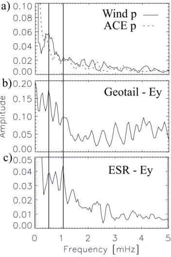
global cavity modes associated with substorm activity (Sam-son et al., 1992; S´anchez et al., 1997), others have suggested that they are externally driven by solar wind pressure (Kepko and Spence, 2003) and/or IMF changes (Mishin et al., 2002). Figure 13 displays the power frequency spectra of the solar wind pressure, the duskward electric field measured by Geo-tail and the reconnection electric field from the ESR data. Although the signal is fairly weak, the Wind measurements show a distinct peak at 0.5 mHz in agreement with Kepko and Spence (2003). In addition to the peak at 1.0 mHz the elec-tric fields measured by Geotail and ESR both show peaks at lower frequencies, 0.5 and 0.8 mHz. As these frequencies are below the lower limit (∼1 mHz) that can be related to cavity modes and internal wave speed (Kepko and Spence, 2003), these results lend support to the possibility that the solar wind pressure can be the driver of these oscillations. To summarize, we find no strong connection between the solar wind electric field and the reconnection rate in the magneto-tail. This leads us to believe that magnetotail reconnection is an internal magnetospheric process. On the other hand, based
ESR - Ey
Wind p
ACE p
a)
b)
Geotail - Ey
c)
Fig. 13. Average power spectrum over the time interval 17:00–
22:00 UT, 7 December 2000, of (a) the solar wind pressure, (b) duskward electric field measured by Geotail and (c) reconnection electric field measured by ESR. Vertical lines mark the cavity mode at 1 mHz and the solar wind pressure variations at 0.5 mHz.
on the power spectra we cannot rule out that the solar wind pressure may modulate the process and impose oscillations modes at low frequencies, in addition to internal magneto-spheric modes.
7 Conclusion
In this paper we have reported how the ion flow across the open-closed boundary can be used to estimate the re-connection electric field in the magnetotail. When guided and confirmed by global imaging by IMAGE FUV we have shown that the electron temperature measurements by the incoherent-scatter EISCAT radars can be used to identify the open-closed boundary. Determination of the orientation of the boundary was based on global imaging by IMAGE FUV. During the two days of observations from the EISCAT radars in Tromsø and on Svalbard we have found:
1) The magnetotail reconnection electric field is not steady but oscillates with a period of 10–15 min between 0 mV/m
and 1 mV/m. The ULF oscillations, which have been found to be a characteristic oscillation mode of the magnetosphere, are mainly due to the motion of the open-closed boundary. Simultaneous in-situ measurements indicate that these oscil-lations extend through large parts of the magnetosphere.
2) Bursts of increased magnetotail reconnection electric field do not necessarily have any auroral signature.
3) The reconnection rate shows poor correlation with the solar wind electric field. This indicates that the magnetotail reconnection is not a directly driven process, but an internal magnetospheric process. Estimates of a coupling efficiency between the solar wind electric field and magnetotail recon-nection give no consistent results and only seem to be rele-vant when averaged over long time intervals. Power spectra indicate that the solar wind pressure may modulate this pro-cess by imposing oscillations modes, in addition to internal modes.
Acknowledgements. We want to thank T. Phan for useful
discus-sions and S. Frey for performing the field line mapping of the EISCAT radar beam locations. The IMAGE FUV investigations were supported by NASA through SwRI subcontract number 83 820 at the University of California at Berkeley under contract number NAS5-96 020. EISCAT is an international association supported by Finland (SA), France (CNRS), Germany (MPG), Japan (NIPR), Norway (NFR), Sweden (NFR), and the United Kingdom (PPARC). J. Moen and K. Oksavik are supported by the Norwegian Research Council and AFOSR task 2311AS. We acknowledge the World Data Center for Geomagnetism (T. Kamei), Kyoto, Japan for providing the preliminary Quick look AE, AL and AU indices and provisional Dst index. Solar wind data were obtained from the CDAweb. We acknowledge the following PIs: Wind Magnetic Field Investigations, R. Lepping; Wind Solar Wind Experiment, K. Ogilvie; ACE/SWEPAM Solar Wind Experiment, D. J. McComas and CE Magnetic Field Instrument, N. Ness. Topical Editor T. Pulkkinen thanks L. Lyons and another refereee for their help in evaluating this paper.
References
Angelopoulos, V., Baumjohann, W., Kennel, C. F., Coroniti, F. V., Kivelson, M. G., Pellat, R., Walker, R. J., L¨uhr, H., and Paschmann, G.: Bursty bulk flows in the inner central plasma sheet, J. Geophys. Res., 97, 4027–4039, 1992.
Blanchard, G. T., Lyons, L. R., de la Beaujardi´ere, O., Doc, R. A., and Mendillo, M.: Measurements of the magnetotail reconnec-tion rate, J. Geophys. Res., 101, 15 265–15 276, 1996.
Blanchard, G. T., Lyons, L. R., and de la Beaujardi´ere, O.: Mag-netotail reconnection rate during magnetospheric substorms, J. Geophys. Res., 102, 24 303–24 312, 1997.
de la Beaujardi´ere, O., Lyons, L. R., and Friis-Christensen, E.: Son-drestrom radar measurements of the reconnection electric field, J. Geophys. Res., 96, 13 907–13 912, 1991.
Doe, R. A., Vickrey, J. F., Weber, E. J., Gallagher, H. A., and Mende, S. B.: Ground-based signatures for the nightside polar cap boundary, J. Geophys. Res., 102, 19 989–20 005, 1997. Dungey, J. W.: Interplanetary magnetic field and the auroral zones,
Fairfield, D. H., Mukai, T., Brittnacher, M., Reeves, G. D., Kokubun, S., Parks, G. K., Nagai, T., Matsumoto, H., Hashimoto, K., Gurnett, D. A., and Yamamoto, T.: Earthward flow bursts in the inner magnetotail and their relation to auroral brightening, AKR intensifications, geosynchrono us particle in-jections and magnetic activity, J. Geophys. Res., 104, 355–370, 1999.
Frey, H. U., Mende, S. B., Immel, T. J., G´erard, J. C., Hubert, B., Spann, J., Gladstone, G. R., Bisikalo, D. V., and Shematovich, V. I.: Summary of quantitative interpretation of IMAGE ultravi-olet auroral data, Space Sci. Rev., 109, 255–283, 2003.
Fujii, R., Hoffman, R. A., Anderson, P. C., Craven, J. D., Sugiura, M., Frank, L. A., and Maynard, N. C.: Electrodynamic parame-ters in the nighttime sector during auroral substorms, J. Geophys. Res., 99, 6187–6199, 1994.
Hesse, M., Schindler, K., Birn, J., and Kuznetsova, M.: The diffu-sion region in collidiffu-sionless magnetic reconnection, Phys. Plasma, 6, 1781, 1999.
Hoffman, R. A., Fujii, R., and Sugiura, M.: Characteristics of the field-aligned current system in the nighttime sector during auro-ral substorms, J. Geophys. Res., 21, 21 303–21 326, 1994. Horton, W. and Doxas, I.: A low-dimension energy-conserving
state space model for substorm dynamics, J. Geophys. Res., 101, 27 223–27 237, 1996.
Kagan, L. M., Kelley, M. C., and Doe, R. A.: Ionosphereic electron heating by structured electric fields: Theory and experiment, J. Geophys. Res., 101, 10 893–10 907, 1996.
Kelley, M. C.: The Earth’s Ionosphere Plasma Physics and Electro-dynamics, Academic Press, Inc., San Diego, 1989.
Kepko, L. and Spence, H. E.: Observations of discrete, global magnetospheric oscillations directly driven by solar wind den-sity variations, J. Geophys. Res., 108, 1257, 2003.
Lockwood, M.: Identifying the open-closed field line boundary, in Polar cap boundary phenomena, edited by J. Moen, A. Egeland, and M. Lockwood, pp. 73–90, Kluwer Academic Publishers in cooperation with NATO Scientific Affairs Division, Dordrecht, Boston, London, 1997.
Lyons, L., Zesta, E., Xu, Y., S´anchez, E. R., Samson, J. C., Reeves, G. D., Ruohoniemi, J. M., and Sigwarth, J. B.: Auroral poleward boundary intensifications and tail bursty flows: A manifestation of a large-scale ULF oscillation?, J. Geophys. Res., 107, 1352, 2002.
Mende, S. B., Heetderks, H., Frey, H. U., Lampton, M., Geller, S. P., Abiad, R., Siegmund, O. H. W., Tremsin, A. S., Spann, J., Dougani, H., Fusilier, S. A., Magoncelli, A. L., Bumala, M. B., Murphree, S., and Trondsen, T.: Far ultraviolet imaging from the IMAGE spacecraft. 2. Wideband FUV imaging, Space Sci. Rev., 91, 271–285, 2000.
Mishin, E. V., Foster, J. C., Potekhin, A. P., Rich, F. J., Schlegel, K., Yumoto, K., Taran, V. I., Ruohoniemi, J. M., and Friedel, R.: Global ULF disturbances during a stormtime substorm on 25 September 1998, J. Geophys. Res., 107, 1486, 2002.
Nakamaura, R., Baumjohan, W., Sergeev, M. B. V., Kubyshkina, M., Mukai, T., and Liou, K.: Flow burst and auroral activa-tions: Onset timing and foot point location, J. Geophys. Res., 106, 10 777 (2000JA000 249), 2001.
Ober, D. M., Maynard, N. C., Burke, W. J., Peterson, W. K., Sig-warth, J. B., Frank, L. A., Scudder, J. D., Hughes, W. J., and Russell, C. T.: Electrodynamics of the poleward auroral border observed by Polar during a substorm on April 22, 1998, J. Geo-phys. Res., 106, 5927–5943, 2001.
Pedersen, A., Catelli, C. A., F¨althammar, C. G., Knott, K., Lindqvist, P. A., Manka, R. H., and Mozer, F. S.: Electric fields in the plasma sheet and plasma sheet boundary, J. Geophys. Res., 90, 1231, 1985.
Russell, C. T.: The configuration of the magnetosphere, in Critical Problems of Magnetospheric Physics, edited by E. R. Dyer, pp. 1–16, National Academy of Sciences, Washington D.C., 1972. Samson, J. C., Lyons, L. R., Newell, P. T., Creutzberg, F., and Xu,
B.: Proton aurora and substorm intensifications, Geophys. Res. Lett., 19, 2167–2170, 1992.
S´anchez, E. R., Kelly, J. D., Angelopoulos, V., Hughes, T., and Singer, H.: Alv´en modluation of the substorm magnetotail trans-port, Geophys. Res. Lett., 24, 979–982, 1997.
Tsyganenko, N. A.: A model of the near magnetosphere with a dawn-dusk asymmetry 1. Mathematical structure, J. Geophys. Res., 107, 1179, 2002.
Vasyliunas, V. M.: Steady state aspects of magnetic field line merg-ing, in Magnetic Reconnection in Space and Laboratory Plasmas, Geophys. Monogr. Ser., vol. 30, edited by E. W. Hones, Jr., pp. 25–31, AGU, Washington, D. C., 1984.
Yamade, Y., Fujimoto, M., Yokokawa, N., and Nakamura, M. S.: Field-aligned currents generated in magnetotail reconnection, Geophys. Res. Lett., 27, 1091, 2000.