HAL Id: hal-00299217
https://hal.archives-ouvertes.fr/hal-00299217
Submitted on 15 Nov 2004
HAL is a multi-disciplinary open access
archive for the deposit and dissemination of
sci-entific research documents, whether they are
pub-lished or not. The documents may come from
teaching and research institutions in France or
abroad, or from public or private research centers.
L’archive ouverte pluridisciplinaire HAL, est
destinée au dépôt et à la diffusion de documents
scientifiques de niveau recherche, publiés ou non,
émanant des établissements d’enseignement et de
recherche français ou étrangers, des laboratoires
publics ou privés.
Correlation analysis technique revealing ionospheric
precursors of earthquakes
S. A. Pulinets, T. B. Gaivoronska, A. Leyva Contreras, L. Ciraolo
To cite this version:
S. A. Pulinets, T. B. Gaivoronska, A. Leyva Contreras, L. Ciraolo. Correlation analysis technique
re-vealing ionospheric precursors of earthquakes. Natural Hazards and Earth System Science, Copernicus
Publications on behalf of the European Geosciences Union, 2004, 4 (5/6), pp.697-702. �hal-00299217�
SRef-ID: 1684-9981/nhess/2004-4-697 © European Geosciences Union 2004
Natural Hazards
and Earth
System Sciences
Correlation analysis technique revealing ionospheric precursors
of earthquakes
S. A. Pulinets1, T. B. Gaivoronska2, A. Leyva Contreras1, and L. Ciraolo3 1Institute of Geophysics, UNAM, Mexico City, Mexico
2Institute of Terrestrial Magnetism, Ionosphere and Radiowave Propagation, RAS, Troitsk, Russia 3Institute of Applied Physics, CNR, Florence, Italy
Received: 1 July 2004 – Revised: 29 October 2004 – Accepted: 9 November 2004 – Published: 15 November 2004 Part of Special Issue “Precursory phenomena, seismic hazard evaluation and seismo-tectonic electromagnetic effects”
Abstract. In this paper we focus on the variability of electron
concentration in the ionosphere measured by ground based ionosondes and GPS receivers around the time of strong earthquakes. It has been detected and statistically proven that several days before the seismic shock the level of this variability increases at the station closest to the epicenter, a fact which can be regarded as precursory phenomenon. More precisely the localness of this specific kind of ionospheric variability is used for the correlation analysis of data of sev-eral observation points. The similarity of geographical loca-tion of the observaloca-tion points leads to the similarity of iono-spheric variations registered at these sites during both quiet and disturbed geomagnetic conditions, except in the case of those located at the seismoactive zone. As a rule, the local anomalies in the F2 layer and TEC accompanying the prepa-ration of strong earthquakes show themselves in the break-ing of the mutual correlation of the critical frequencies foF2
or TEC between stations situated in and outside the seismic zone. The precursory phenomenon appears 1 to 7 days be-fore the time of the seismic shock.
1 Introduction
In short-term earthquake prediction two principal directions can be separated. First one – the deterministic approach which studies the temporal and spatial distribution behavior of some precursor, for example, the radon emanation (Allegri et al., 1983; King et al., 1993). The other one – the statistical patterns processing on the purpose to find some regularity in the behavior of statistical characteristics of the given param-eter. Self organized criticality is one of the main streams of statistical earthquake prediction at the present moment (Run-dle et al., 2000).
It was established recently that seismic activity is one of the sources of the day-to-day ionospheric variability
(Pu-Correspondence to: S. A. Pulinets
linets, 1998; Pulinets and Boyarchuk, 2004; Pulinets and Liu, 2004; Liu et al., 2004). The coupling between the ground surface and the ionosphere is due to the anomalous electric field generated in the earthquake preparation area (Pulinets et al., 2000). The earthquake preparation area conception was introduced by Dobrovolsky et al. (1979) using the elastic de-formation calculations. The size of the earthquake prepara-tion area depends on the earthquake magnitude. The same (or very similar) dependencies were obtained not only in the case of the elastic deformations, but also in that of the spa-tial distribution of different types of precursors in the seis-mic activation zone (Bowman et al., 1998; Kossobokov et al., 2000) including geochemical ones (Toutain and Baubron, 1999) and local seismicity. Penetrating the ionosphere the anomalous electric field causes the ion drift that results in the formation of electron density irregularities (Kim and Hegai, 1997). These anomalies that appear in the ionosphere before the main seismic shock can be considered as ionospheric pre-cursors (Pulinets and Boyarchuk, 2004). The existence of the ionospheric anomalies/ionospheric precursors is well estab-lished not only by physical modeling but statistically as well (Pulinets et al., 2002; Liu et al., 2004; Chen et al., 2004).
For the ionospheric precursors of earthquakes, both ap-proaches are used. One way is to track the specific iono-sphere parameters trying to detect in the measurements the recently revealed main features of the ionospheric precursor (Pulinets et al., 2003). The other way is to use the statisti-cally established behavior of some parameter (for example, the critical frequency foF2) as a signature of the
impend-ing earthquake (Pulinets et al., 2002). Both approaches have their advantages as well as their drawbacks. The first method could fail in magnetically disturbed conditions, while the second requires an a priori knowledge of the precursor be-havior, which must be acquired through many years of ob-servations. Obviously, this amount of information will be unattainable for locations with recently installed ionosonde or GPS receiver.
For the present study, one of the most important charac-teristics of the ionospheric precursors of earthquakes is their
698 S. A. Pulinets et al.: Correlation analysis technique revealing ionospheric precursors of earthquakes
12 Figure 1.Configuration of the measurement points positions and earthquake preparation area for the correlation technique described in the paper.
Fig. 1. Configuration of the measurement points positions and earthquake preparation area for the correlation technique described in the paper.
local character. The localness of seismo-ionospheric vari-ations has been demonstrated by different techniques, being the most effective the topside sounding that shows the config-uration of the modified areas in the ionosphere, their size and temporal dynamics (Pulinets and Legen’ka, 2003). The size of the modified area in the ionosphere is of the same order of magnitude as the size of the earthquake preparation area on the ground surface (Dobrovolosky, 1979; Pulinets et al., 2004). This fact offers us an opportunity to propose a very simple but quite effective technique of detecting the iono-spheric variations associated with the earthquake preparation process.
2 Description of the technique
In the simplest configuration two measurement points are used: one (“receiver-sensor”) located inside the earthquake preparation area (see Fig. 1), and the other (“control-receiver”) located outside it.
Two important considerations regarding receivers localiza-tion are taken into account
1. receivers should be in the same (or very close) geomag-netic latitude, in order to ensure the similarity of their reaction to geomagnetic disturbances.
2. the longitude of the receivers should not differ too much because of the LT (local time) dependence of iono-sphere reaction to geomagnetic storm commencement. In general, the ionospheric variability in terms of critical frequency variations is lower for those variations associated with seismic activity than for those associated with geomag-netic storms. Therefore, the seismically generated variations may be shadowed by the storm-time variations. However, if two measurement points are used with the configuration shown in Fig. 1, storm-time variations can be excluded by cross-correlation of the records at the given points as storm-time variations will be practically identical for both stations. It has been shown (Szuszczewisz et al., 1998) that in a large
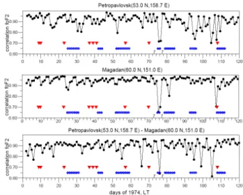
13 Figure 2. From top to bottom: autocorrelation coefficient for Petropavlovsk ionospheric station, autocorrelation coefficient for Magadan ionospheric station, cross-correlation coefficient between Petropavlovsk and Magadan stations for period January-April 1974. Triangles indicate the days with earthquakes, diamonds – magnetically disturbed days. Fig. 2. From top to bottom: autocorrelation coefficient for Petropavlovsk ionospheric station, autocorrelation coefficient for Magadan ionospheric station, cross-correlation coefficient between Petropavlovsk and Magadan stations for period January-April 1974. Triangles indicate the days with earthquakes, diamonds – magneti-cally disturbed days.
range of latitudes and longitudes the ionospheric reaction to geomagnetic disturbances is very similar (see Fig. 3 in Szuszczewisz et al., 1998), and this may provide high cor-relation in the daily variations between different ionospheric stations. At a given time, the “receiver sensor” will be much more sensitive to the seismogenic variations in comparison with the “control receiver”. This fact is used in the proposed technique.
For the calculation of the daily correlation coefficients we use the standard definition of the cross-correlation coefficient (Devore, 2000) where the records of the critical frequency, or vertical total electron content (TEC), with equal time inter-vals for the given day are used:
C = P i=0,k (f1,i−af1)(f2,i−af2) k(σ1σ2) .
The indices 1 and 2 correspond to the first and second iono-spheric station(s), f = foF2 (hourly values of the critical
frequency scaled from the ionograms), k=23 and af and σ are determined by the following expressions (in principle, other sampling intervals can be used, for example 15 min intervals as it is used at ionospheric stations, or 10 min in-tervals, which we use for vertical TEC calculations, respec-tively, k will correspond to the number of records):
af = P i=0,k fi k +1 σ2= P i=0,k (fi −af )2 k
14 Figure 3 Upper panel - cross-correlation coefficient for Petropavlovsk and Magadan stations for period January-April 1992. Bottom panel M and m coefficients for the same stations and the same period. Triangles indicate the days with earthquakes, crosses – magnetically disturbed days. 0 10 20 30 40 50 60 70 80 90 100 110 120 days LT, January-April 1992 0.5 0.6 0.7 0.8 0.9 1.0 C f oF2 Petropavlovsk(53.0N,158.7E)-Magadan(60.0N,151.0E) 0 10 20 30 40 50 60 70 80 90 100 110 120 days LT, January-April 1992 -5.0 0.0 5.0 mM f oF2, MHz Petropavlovsk(53.0N,158.7E)-Magadan(60.0N,151.0E)
Fig. 3. Upper panel – cross-correlation coefficient for Petropavlovsk and Magadan stations for period January–April 1992. Bottom panel M and m coefficients for the same stations and the same period. Triangles indicate the days with earthquakes, crosses – magnetically disturbed days.
af is a daily mean value of the critical frequency, σ is the standard deviation.
3 The hypothesis testing
The proposed technology was tested on the series of earth-quakes in the Western Pacific area (Russia Far East, Taiwan, Japan). As an example we will consider the data of two Russian stations: Petropavlovsk-na-Kamchatke (53.0◦N,
158.7◦E) and Magadan (60.0◦N, 151.0◦E). The first one
is inside the main Russian seismoactive area – Kamchatka peninsula. To demonstrate the “clearing process” we present the autocorrelation coefficients of both stations for a period of 4 months (January–April, 1974) in the upper two panels of the Fig. 2. Autocorrelation means that every consequent day was correlated with the preceding one. Every magnetic disturbance causing a change in the daily variation of the crit-ical frequency would be tracked by each station in the form of the drop of the autocorrelation coefficient. However, due to increased ionospheric variability caused by the seismic activation mentioned in Introduction, the additional drops of autocorrelation coefficient appeared only on the record of Petropavlovsk station, because of its location inside the earthquake preparation area. The cross-correlation is shown in the bottom panel of Fig. 2. One can see that, at least during the first part of the observed period, only the drops connected with the seismic events are left at the cross-correlation coef-ficient records in comparison with autocorrelation records. A similar pattern can be observed for another period (January– April 1992) in the upper panel of the Fig. 3. In both cases (Figs. 2 and 3) the drops of the cross-correlation coefficient happened from 5 to 7 days before the time of the seismic shock.
Another parameter that can be used for estimating the spa-tial ionospheric variability is the daily maximum and mini-mum difference of the critical frequencies hourly values of both stations (Gaivoronskaya and Pulinets, 2002):
M =max {f1,i−f2,i}i=0,k
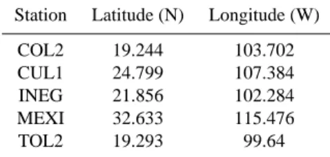
Table 1. Coordinates of INEGI GPS receivers used for the analysis
of GPS TEC around the time of Colima earthquake.
Station Latitude (N) Longitude (W)
COL2 19.244 103.702
CUL1 24.799 107.384
INEG 21.856 102.284
MEXI 32.633 115.476
TOL2 19.293 99.64
m =min {f1,i−f2,i}i=0,k.
It is obvious that the larger difference between indices M and m means the increased variability. Sometimes (like in equinoctial conditions), when the daily maximum of the crit-ical frequency is not so expressed due to extension of day-light hours, the use of these indices of the variability can be even more effective, a fact which is demonstrated at the bot-tom panel of Fig. 3. It can be seen from the figure that the instability observed in April in upper panel disappeared in the bottom one, but precursory effects are seen in the figure as well.
4 The technique testing by GPS TEC data
It has been shown (Liu et al., 2001) that the correlation coef-ficient between the variations of the peak electron concen-tration N mF 2 and vertical TEC (Total Electron Content) is 0.953, including in periods of anomalous variations con-nected with seismic activity. This opens the possibility of applying the developed technique to the TEC variations de-rived from the GPS receivers network. Such attempt was made for the recent strong (Mw=7.8) Colima earthquake in
Mexico, occurred on 21 January (20:06:48.09 LT), or 22 Jan-uary (02:06:48.09 GMT) of 2003.
To detect the possible ionospheric variations associated with this earthquake the data of 5 stationary GPS receivers of the National Institute of Statistics, Geography and Informat-ics (INEGI) were used. The stations coordinates are shown in Table 1.
The data of the closest to epicenter receiver (COL2) were analyzed first. To this purpose the monthly median was cal-culated to compare with current data, and to determine the deviations from the monthly median. Results are shown in Fig. 4. For the better time resolution only several days around the time of the Colima earthquake are shown, clearly demon-strating the presence of anomalous variations out of the upper bound on 18 and 19 of January.
The current observations are indicated with a thick line, and represent the vertical TEC in TEC units (1 TECu=1016el/m2). Monthly mean is indicated with a thin line, and the upper bound with a dashed one. For the time when anomalous peak of TEC was registered on 18 January (10:10 LT on 18 January 2003), the map of the TEC deviation
700 S. A. Pulinets et al.: Correlation analysis technique revealing ionospheric precursors of earthquakes
15 Figure 4 Vertical TEC variations (points) in comparison with the monthly mean (thick line). Thin line – upper bound calculated as monthly mean + Fig. 4. Vertical TEC variations (points) in comparison with theσ.
monthly mean (thick line). Thin line – upper bound calculated as monthly mean +σ .
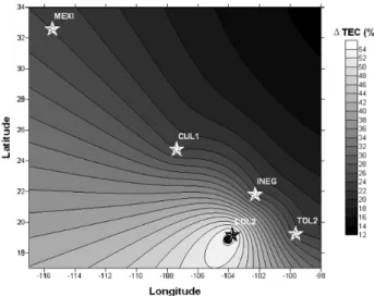
16 Figure 5 Spatial distribution of the vTEC deviation from the monthly median at 1010 LT 18 January 2003
Fig. 5. Spatial distribution of the vTEC deviation from the monthly
median at 10:10 LT on 18 January 2003.
from the monthly median was constructed (Fig. 5) using the data of 5 receivers (their coordinates are shown in Table 1). Acknowledging the limitations of such map (low spatial res-olution, lack of measurements in the left bottom corner of the map, which is in the Pacific Ocean) it clearly demon-strates the presence of an anomaly just around the epicenter position of the impending earthquake. Keep in mind that dis-tribution is built for a period of time of more than 3 days before the seismic shock.
To determine whether the correlation technique works for the GPS data, the cross-correlation coefficient between dif-ferent stations was calculated. Taking into account that Col-ima receiver stopped measurements immediately after the seismic shock, due to damage and incompleteness of data records on 17 January (important day for the precursors iden-tification), the Toluca receiver (TOL2) was used as a “sensor” station. In Fig. 6 the cross-correlation coefficients for the pairs TOL2-INEG and TOL2-CUL are presented. The drop
17 1 2 3 4 5 6 7 8 9 10 11 12 13 14 15 16 17 18 19 20 21 22 23 24 25 26 27 28 29 30 31 January, 2003 (UT) 0.6 0.7 0.8 0.9 1 co rr (c u l_t o l2 ) 0 2 4 6 8 10 12 14 16 18 20 22 24 26 28 30 January, 2003 (UT) 0.6 0.7 0.8 0.9 1 co rr (i n e g _to l2 )
Figure 6 Daily cross-correlation coefficients for vertical TEC derived from data of Toluca (TOL2), Culiacan (CUL) and Aguascalientes (INEG) receivers for the period around the time of Colima earthquake. Upper panel – correlation coefficient between Culiacan and Toluca stations, bottom panel – correlation coefficient between Aguascalientes and Toluca stations. The time of the Colima earthquake is indicated in figures by sign
Fig. 6. Daily cross-correlation coefficients for vertical TEC
de-rived from data of Toluca (TOL2), Culiacan (CUL) and Aguas-calientes (INEG) receivers for the period around the time of Colima earthquake. Upper panel – correlation coefficient between Culiacan and Toluca stations, bottom panel – correlation coefficient between Aguascalientes and Toluca stations. The time of the Colima earth-quake is indicated in figures by sign.
of the correlation coefficient 5 days before the seismic shock in the both panels and a smaller drop, 7 and 8 days before the shock respectively, can be seen.
As one can see, the correlation technique works for GPS TEC data as well. It shows the same time scale for precur-sors as for the vertical sounding: precurprecur-sors appear 5 days before the seismic shock as it was described by Pulinets et al. (2003). The high correlation between the stations records is violated within the period several days before strong seis-mic shock.
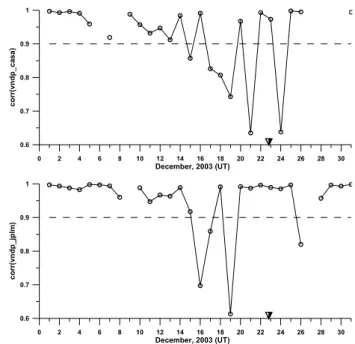
The second fast check of the correlation technique was made for the San Simeon earthquake in central California in December 2003: M=6.5, 35.7◦N, 121.1◦W, 19:15:56 GMT on 22 December 2003. The map of the GPS receivers used for the analysis and the epicenter position are shown in Fig. 7. The receiver closest to the epicenter (VNDP) is used as a “sensor”. The graphs of the correlation coefficient for 3 sta-tions are shown in Fig. 8. Both curves indicate the gradual drop of the cross-correlation coefficient starting from 15 of December, i.e. 7 days before the shock with absolute minima registered one day and three days before the shock respec-tively. CASA indicates a minimum the day after the shock which can be associated with the acoustic action of the shock on the ionosphere. It should be noted that not all the stations from Fig. 7 showed the drop of the correlation coefficient, which indicates the dependence of the technique on the re-ceiver position. The reason of this fact was explained by Pu-linets et al. (2004) and is connected with the complex
distri-18 Figure 7 Positions of GPS receivers (stars) used in analysis of TEC variations around the time
of San Simeon earthquake 22 December 2003. - earthquake epicenter position
Fig. 7. Positions of GPS receivers (stars) used in analysis of TEC
variations around the time of San Simeon earthquake 22 December 2003. Earthquake epicenter position.
bution of electron concentration anomaly in the ionosphere. It could happen that the station does not “feel” the anomaly at all, as sometimes happens in our correlation analysis. This question needs more careful investigation, and is the purpose of a future work. Such study demands a very dense network of GPS receivers, but at the time only Japan and the State of California (USA) have enough receivers to provide the nec-essary resolution.
5 Conclusions
Very simple but powerful technique was presented which is based on the correlation of records of two receiving sta-tions (ionosondes or GPS receivers). One of them is situated within the area of earthquake preparation, while the other one (being in the same geophysical conditions) is outside the earthquake preparation area (or its outer edge). Due to similar geophysical conditions the correlation coefficient for the registering stations is very high (usually, more than 0.9), but few days before the strong seismic shock (from 7 to 1) sharp drops of the daily correlation coefficient appear man-ifesting the increased variability of the ionosphere over the earthquake preparation area. The proposed technique per-mits to identify the ionospheric precursors even in geomag-netically disturbed conditions. The other parameters which can be used for ionosphere variability estimation is the differ-ence between maximal and minimal daily values of the criti-cal frequency foF2 (or vertical TEC) for the stations used in
correlation analysis.
Some limitation of the proposed technique is connected with the fact that an arbitrary location of the “sensor” station
19 0 2 4 6 8 10 12 14 16 18 20 22 24 26 28 30 December, 2003 (UT) 0.6 0.7 0.8 0.9 1 co rr (v n d p _ca sa) 0 2 4 6 8 10 12 14 16 18 20 22 24 26 28 30 December, 2003 (UT) 0.6 0.7 0.8 0.9 1 co rr (v nd p_ jp lm )
Figure 8 Daily cross-correlation coefficients for vertical TEC derived from GPS receivers network at California, USA for December 2003. Upper panel – correlation coefficient between VNDP and CASA stations, bottom panel – correlation coefficient between VNDP and JPLM stations. The time of the San Simeon earthquake is indicated in figures by sign. The stations and the epicenter positions are shown in the map (Figure 7).
Fig. 8. Daily cross-correlation coefficients for vertical TEC
de-rived from GPS receivers network at California, USA for Decem-ber 2003. Upper panel – correlation coefficient between VNDP and CASA stations, bottom panel – correlation coefficient between VNDP and JPLM stations. The time of the San Simeon earthquake is indicated in figures by sign. The stations and the epicenter posi-tions are shown in the map (Fig. 7).
may not give the positive result. This fact is connected with the complex configuration of anomalous variations within the ionosphere. The ionospheric irregularity may be shifted along the geomagnetic field lines equatorward against the vertical projection of the epicenter of the impending earth-quake on the ionosphere. In such a situation the “sensor” station becomes blind and cannot “feel” the anomalous vari-ations. This situation may be avoided by an accurate selec-tion of the posiselec-tions of the “sensor” and “control” staselec-tions. It requires the additional investigations within the particu-lar zone of seismic activity. Nevertheless the proposed tech-nique permits a low cost monitoring of ionospheric precur-sors of earthquakes avoiding the use of expensive satellite technologies.
Acknowledgements. This work was supported by the grants of PAPIIT IN 126002, and CONACYT 40858-F. The authors thank the Mexican National Institute of Statistics, Geography and Informatics (INEGI) for providing the GPS data from their network. Edited by: M. Contadakis
702 S. A. Pulinets et al.: Correlation analysis technique revealing ionospheric precursors of earthquakes
References
Allegri, L., Bella, F., Delia Monica, G., Ermini, A., Impora, S., Sgrigna, V., and Biagi, P. F.: Radon and tilt anomalies detected before the Irpinia (South Italy) earthquake of 23 November 1980 at great distance from the epicenter, Geophys. Res. Lett., 10, 269–272, 1983.
Bowman, D. D., Ouillon, G., Sammis, C. G., Sornette, A., and Sor-nette, D.: An observation test of the critical earthquake concept, J. Geophys. Res., 103, 24 359–24 372, 1998.
Chen, Y. I., Liu, J. Y., Tsai, Y. B., and Chen, C. S.: Statistical tests for pre-earthquake ionospheric anomaly, Terr. Atm. Ocean Sci., 15, 385–396, 2004.
Devore, J. L.: Probability and Statistics for Engineering and the Sciences, Duxbury Thomson Learning, USA, 775, 1999. Dobrovolsky, I. R., Zubkov, S. I., and Myachkin, V. I.:
Estima-tion of the size of earthquake preparaEstima-tion zones, Pageoph., 117, 1025–1044, 1979.
Gaivoronskaya, T. V. and Pulinets, S. A.: Analysis of F2-layer vari-ability in the areas of seismic activity, Preprint IZMIRAN No. 2(1145) Moscow, 20, 2002.
Kim, V. P. and Hegai, V. V.: On possible changes in the midlatitude upper ionosphere before strong earthquakes, J. Earthq. Predict. Res., 6, 275–280, 1997.
King, C.-Y., Zhang, W., and King, B.-S.: Radon Anomalies on Three Kinds of Faults in California, Pageoph., 141, 111–124, 1993.
Kossobokov, V. G., Keilis-Borok, V. I., Turcotte, D. L., and Mala-mud, B. D.: Implications of a Statistical Physics Approach for Earthquake Hazard Assessment and Forecasting, Pure Appl. Geophys., 157, 2323–2349, 2000.
Liu, J. Y., Chen, Y. I., Chuo, Y. J., and Tsai, H. F.: Variations of ionospheric total electron content during the Chi-Chi earthquake, Geophys. Res. Lett., 28, 1383–1386, 2001.
Liu, J. Y., Chuo, Y. J., Shan, S. J., Tsai, Y. B., Pulinets, S. A., and Yu, S. B.: Pre-earthquake ionospheric anomalies monitored by GPS TEC, Ann. Geophys., 22, 1585–1593, 2004,
SRef-ID: 1432-0576/ag/2004-22-1585.
Pulinets, S. A.: Seismic activity as a source of the ionospheric vari-ability, Adv. Space Res., 22, 903–906, 1998.
Pulinets, S. A., Boyarchuk, K. A., Khegai, V. V., Kim, V. P., and Lomonosov, A. M.: Quasielectrostatic Model of Atmosphere-Thermosphere-Ionosphere Coupling, Adv. Space Res., 26, 1209– 121, 2000.
Pulinets, S. A., Boyarchuk, K. A., Lomonosov, A. M., Khegai, V. V., and Liu, J. Y.: Ionospheric precursors to earthquakes: a
preliminary analysis of the foF2 critical frequencies at
Chung-Li ground-based station for vertical sounding of the ionosphere (Taiwan island), Geomagnetism and Aeronomy, 42, 508–513, 2002.
Pulinets, S. A. and Legen’ka, A. D.: Spatial-temporal character-istics of the large scale disturbances of electron concentration observed in the F-region of the ionosphere before strong earth-quakes, Cosm. Res., 41, 221–229, 2003.
Pulinets, S. A., Legen’ka, A. D., Gaivoronskaya, T. V., and Depuev, V. Kh.: Main phenomenological features of ionospheric precur-sors of strong earthquakes, J. Atmos. Solar-Terr. Phys., 65, 1337– 1347, 2003.
Pulinets, S. A. and Boyarchuk, K. A.: Ionospheric Precursors of Earthquakes, Springer, Berlin, Germany, 315, 2004.
Pulinets, S. A., Liu, J. Y., and Safronova, I. A.: Interpretation of
a statistical analysis of variations in the foF2 critical frequency
before earthquakes based on data from Chung-Li ionospheric sta-tion (Taiwan), Geomagn. Aeronom., 44, 102–106, 2004. S. A. Pulinets and Liu, J. Y.: Ionospheric variability unrelated to
solar and geomagnetic activity, Adv. Space Res., 34, 1926–1933, 2004.
Rundle, J. B., Turcotte, D. L., and Klein W. (eds.): GeoComplexity and the Physics of Earthquakes, Geophysical Monographs Se-ries, American Geophysical Union, Washington D. C., 2000. Szuszczewicz, E. P., Lester, M., Wilkinson, P., Blanchard, P., Abdu,
M., Hanbaba, R., Igarashi, K., Pulinets, S., and Reddy, B. M.: Global ionospheric storm characteristics during solar maximum equinox, J. Geophys. Res., 103, 11 665–11 684, 1998.
Toutain, J.-P. and Baubron, J.-C.: Gas geochemistry and seismotec-tonics: a review, Tectonophysics, 304, 1–27, 1998.