HAL Id: hal-02956546
https://hal.archives-ouvertes.fr/hal-02956546
Submitted on 5 Oct 2020
HAL is a multi-disciplinary open access
archive for the deposit and dissemination of
sci-entific research documents, whether they are
pub-lished or not. The documents may come from
teaching and research institutions in France or
abroad, or from public or private research centers.
L’archive ouverte pluridisciplinaire HAL, est
destinée au dépôt et à la diffusion de documents
scientifiques de niveau recherche, publiés ou non,
émanant des établissements d’enseignement et de
recherche français ou étrangers, des laboratoires
publics ou privés.
earthquake from joint inversion of near-field hr-GPS and
teleseismic body wave recordings constrained by
tsunami observations
Han Yue, Thorne Lay, Luis Rivera, Yefei Bai, Yoshiki Yamazaki, Kwok Fai
Cheung, Emma M. Hill, Kerry Sieh, Widjo Kongko, Abdul Muhari
To cite this version:
Han Yue, Thorne Lay, Luis Rivera, Yefei Bai, Yoshiki Yamazaki, et al.. Rupture process of the 2010
Mw 7.8 Mentawai tsunami earthquake from joint inversion of near-field hr-GPS and teleseismic body
wave recordings constrained by tsunami observations. Journal of Geophysical Research : Solid Earth,
American Geophysical Union, 2014, 119 (7), pp.5574-5593. �10.1002/2014JB011082�. �hal-02956546�
Rupture process of the 2010
M
w7.8 Mentawai
tsunami earthquake from joint inversion
of near-
field hr-GPS and teleseismic
body wave recordings constrained
by tsunami observations
Han Yue1, Thorne Lay1, Luis Rivera2, Yefei Bai3, Yoshiki Yamazaki3, Kwok Fai Cheung3, Emma M. Hill4, Kerry Sieh4, Widjo Kongko5, and Abdul Muhari6
1
Department of Earth and Planetary Sciences, University of California, Santa Cruz, California, USA,2Institut de Physique du Globe de Strasbourg, Université de Strasbourg/CNRS, Strasbourg, France,3Department of Ocean and Resources Engineering, University
of Hawaii at Manoa, Honolulu, Hawaii, USA,4Earth Observatory of Singapore, Nanyang Technological University, Singapore,
5Coastal Dynamic Research Center, Indonesian Agency for the Assessment and Application of Technology, Jogjakarta, Indonesia, 6
International Research Institute of Disaster Science, Tohoku University, Sendai, Japan
Abstract
The 25 October 2010 Mentawai tsunami earthquake (Mw7.8) ruptured the shallow portion of the Sunda megathrust seaward of the Mentawai Islands, offshore of Sumatra, Indonesia, generating a strong tsunami that took 509 lives. The rupture zone was updip of those of the 12 September 2007 Mw8.5and 7.9 underthrusting earthquakes. High-rate (1 s sampling) GPS instruments of the Sumatra GPS Array network deployed on the Mentawai Islands and Sumatra mainland recorded time-varying and static ground displacements at epicentral distances from 49 to 322 km. Azimuthally distributed tsunami recordings from two deepwater sensors and two tide gauges that have local high-resolution bathymetric information provide additional constraints on the source process. Finite-fault rupture models, obtained by joint inversion of the high-rate (hr)-GPS time series and numerous teleseismic broadband P and S wave seismograms together with iterative forward modeling of the tsunami recordings, indicate rupture propagation ~50 km up dip and ~100 km northwest along strike from the hypocenter, with a rupture velocity of ~1.8 km/s. Subregions with large slip extend from 7 to 10 km depth ~80 km northwest from the hypocenter with a maximum slip of 8 m and from ~5 km depth to beneath thin horizontal sedimentary layers beyond the prism deformation front for ~100 km along strike, with a localized region having>15 m of slip. The seismic moment is 7.2 × 10²⁰N m. The rupture model indicates that local heterogeneities in the shallow megathrust can accumulate strain that allows some regions near the toe of accretionary prisms to fail in tsunami earthquakes.
1. Introduction
The Australian plate is converging with the southeastern segment of the Eurasian plate, called the Sunda block, at a relative plate motion rate of ~59 mm/yr [Bock et al., 2003; Chlieh et al., 2008]. The plate motion is oblique to the Sumatran subduction zone, with slip partitioning having generated a fore-arc sliver along Sumatra (Figure 1). The boundary-parallel shear motion is mainly accommodated along the Sumatran fault, and the boundary-perpendicular convergent motion is mainly accommodated by underthrusting along the Sunda megathrust at a rate of ~45 mm/yr [Chlieh et al., 2008].
1.1. Recent Sunda Megathrust Earthquakes
During the past decade, much of the Sunda megathrust has slipped in large earthquakes, with the 26 December 2004 Sumatra-Andaman (Mw9.2) and 28 March 2005 Nias (Mw8.6) events rupturing the zone from 0°N to 14°N [Lay et al., 2005; Ammon et al., 2005; Shearer and Bürgmann, 2010]. The subduction interface from 2°S to 5°S, near the Pagai Islands (southeastern Mentawai Islands), subsequently ruptured in three large events. On 12 September 2007, the Mw8.5 Bengkulu and Mw7.9 Pagai-Sipora events (Figure 1) occurred on
the central and deeper portion of the megathrust with seismic moments of M0= 6.7 × 10²¹N m and 8.1 × 10²⁰N m,
respectively [http://www.globalcmt.org/]. The great Bengkulu event had maximum slip of 5–7 m [Konca et al., 2008]
Journal of Geophysical Research: Solid Earth
RESEARCH ARTICLE
10.1002/2014JB011082Key Points:
• The 2010 Mentawai tsunami earthquake ruptured to the trench
• Rupture model is obtained by modeling hr-GPS, seismic, and tsunami data • Patchy slip at the toe of the trench
indicates local strain accumulation
Supporting Information: • Readme • Figure S1 • Figure S2 • Text S1 • Text S2 • Animation S1 • Animation S2 Correspondence to: T. Lay, [email protected] Citation:
Yue, H., T. Lay, L. Rivera, Y. Bai, Y. Yamazaki, K. F. Cheung, E. M. Hill, K. Sieh, W. Kongko, and A. Muhari (2014), Rupture process of the 2010 Mw7.8 Mentawai tsunami earthquake from joint inversion of near-field hr-GPS and teleseismic body wave recordings constrained by tsunami observations, J. Geophys. Res. Solid Earth, 119, 5574–5593, doi:10.1002/ 2014JB011082.
Received 28 FEB 2014 Accepted 11 JUN 2014
Accepted article online 17 JUN 2014 Published online 8 JUL 2014
and generated a moderately damaging tsunami that impacted 250 km along the coast, with peak runup heights of up to 4 m and inundation distances of up to 500 m [Borrero et al., 2009].
On 25 October 2010, an Mw7.8 thrust earthquake ruptured the shallow portion of the Sunda megathrust seaward
of the Pagai Islands (14:42:21.4 UTC, 3.49°S, 100.14°E, Badan Meteorologi, Klimatologi dan Geofisika (BMKG)). Estimates of short-period body wave magnitude (mb= 6.1–6.5) and surface wave magnitude (MS= 7.1–7.6) from various organizations are tabulated by the International Seismological Centre (http://www.isc.ac.uk/iscbulletin/ search/bulletin/). The Global Centroid Moment Tensor (GCMT) solution has M0= 6.8 × 10²⁰N m (Mw7.8;
http://www.globalcmt.org/), with a centroid depth of 12 km, a centroid time shift of 37.3 s, and a best double couple with strikeϕ = 316°, dip δ = 8°, and rake λ = 96°. W phase inversion yielded a seismic moment M0= 5 × 10²⁰N m (Mw7.7) for a 12 km deep source withδ = 10° [Lay et al., 2011b].
Although lower in seismic magnitudes and seismic moment than the 2007 events, the 2010 earthquake produced a stronger tsunami, with 3–9 m runup that inundated as far as 600 m inland on the Pagai Islands. Peak runup of 16.9 m occurred on the small island of Sibigau [Hill et al., 2012]. The tsunami caused widespread destruction that displaced more than 20,000 people and affected about 4000 households; 509 people were killed [Hill et al., 2012]. The unusually large tsunami for a moderate magnitude earthquake (MS≤ 7.6) classifies the 2010 event as a “tsunami earthquake”[Kanamori, 1972]. The 2010 Mentawai
Figure 1. Maps of the study area and regional plate tectonic setting. The inset map locates the Australian plate which subducts beneath the Sunda Block of the Eurasian plate along the Sunda trench. The relative plate motion, referenced to the Sunda block, is marked with black arrows. The Sunda trench is marked with barbed solid line. The Sumatran fault is marked with a black curve with one-sided arrows to represent the shearing motion. A fore-arc sliver is located between the Sunda trench and the Sumatran fault. The epicenter of the 25 October 2010 Mentawai event is marked with a red star.
The box identifies the region that is enlarged in the main map. The Global Centroid Moment Tensor solution is shown for
the 25 October 2010 Mentawai, Mw7.8 event (blackfilled focal mechanism). The slip distribution of the Mentawai event
is indicated with a red-scaled contour map with 6 m slip increment contours. The rupture areas with slip>1 m for the
12 September 2007 Mw= 8.5 and Mw= 7.9 events [Konca et al., 2008] are marked with blue and purplefilled patches,
respectively. The rupture areas of the 1797 and 1833 events are outlined with red and yellow dashed lines, respectively [Chlieh et al., 2008; Natawidjaja et al., 2006]. The approximate location of the trench is indicated with the barbed curve. The Sumatran fault is indicated with a white curve, with one-sided arrows showing shearing motion. The plate motion between
the Australian plate and Sunda block is indicated with whitefilled arrows. Names of some Mentawai Islands, including
earthquake was not strongly felt locally, as has also been the case for other tsunami earthquakes, limiting immediate reaction to the event and exacerbating the losses from tsunami. The weak shaking is associated with the relatively low radiated seismic energy ER= 9.2 × 10¹⁴J (ER/M0= 1.4 × 10 6) and low source strength for
seismic wave periods shorter than 100 s [Lay et al., 2011b]. The location updip of the preceding large 2007 interplate ruptures is of particular significance, as it is often assumed that isolated shallow megathrust ruptures will not occur seaward of deeper underthrusting events and that stable creep or afterslip [e.g., Hsu et al., 2006] will instead accommodate the relative plate motions.
1.2. Historical Earthquakes
The plate interface near the Mentawai Islands ruptured previously in the 1797 (Mw~8.5–8.7) and 1833
(Mw~ 8.6–8.9) events, which had estimated rupture zones (Figure 1) that appear to have overlapped near Sipora and the Pagai Islands [Natawidjaja et al., 2006; Chlieh et al., 2008] along the 2010 Mentawai rupture zone. It is unclear whether the region of overlap of the 1797 and 1833 rupture zones involved repeated slip or along-dip separation of slip. The 1797 event produced uplift of up to 0.8 m on the southwest coast of the Pagai Islands, and the 1833 event produced uplift of ~2 m on the same coast [Natawidjaja et al., 2006], indicating that the downdip limit of slip was northeast of the islands for both events. The estimated magnitudes of the historic events may be amplified by afterslip and backthrusting that augmented uplift of the coral reefs. Whether slip extended to the trench for either event is not well constrained. There is some documentation of tsunami runup, near Padang on the mainland, of ~5–10 m in the 1797 event and 3–4 m in the 1833 event, which is comparable to that of the 2007 Bengkulu event [Natawidjaja et al., 2006], but there are no reports of runup heights on the Mentawai Islands. It is plausible that these two events did rupture the full width of the seismogenic megathrust, given their documented strong shaking and large tsunami. This possibility is weakly supported by modeling of the uplift patterns on the islands, but the observed deformation does not resolve the updip limit of slip for either event. It is also unclear why the 2007 events were smaller than the earlier events (Figure 1) and why the 2010 rupture did not occur at the time of the earlier events.
In ~1314, the area between the Mentawai Islands and the trench ruptured in a shallow thrust event that was larger and/or deeper than the 2010 Mentawai event [Philibosian et al., 2012]. The estimated magnitude of the 1314 event based on modeling of coral microatolls trades off with the slip location, but the event is distinctive from the further downdip 2007 events. At least two shallow paleo-earthquakes also appear to have shocked the shallow portion of the megathrust near the Mentawai Islands ~1500 years before the 1314 event, indicating an earthquake recurrence time of ~1000 years [Philibosian et al., 2012].
The region of the 1797 rupture zone from latitudes 0.5° to 3° that has not ruptured recently is identified as the Mentawai (or Padang) seismic gap and is a shaking and tsunami threat to the Mentawai Islands, the city of Padang, and surrounding coastal areas. With over 200 years of plate motion since the last event, and clear evidence of interplate locking [Chlieh et al., 2008] southeastward from the Batu Islands to the Pagai Islands (along Siberut and Sipora Islands), there is substantial accumulated moment deficit in the Mentawai gap comparable to that released in the 1833 event to the southeast.
1.3. Prior Results for the 2010 Event
The faulting process of the 2010 Mentawai event has been investigated using subsets of seismic, geodetic, and tsunami data sets [Lay et al., 2011b; Newman et al., 2011; Bilek et al., 2011; Hill et al., 2012; Satake et al., 2013]. These prior investigations reveal some consistent characteristics of the tsunami earthquake but differ in estimated slip distribution due to the varying intrinsic resolution provided by each data type and observational configuration.
Teleseismic body and surface wave inversions [Lay et al., 2011b; Newman et al., 2011; Bilek et al., 2011] inferred primary slip patches located near the hypocenter along with overall northwestward along-strike expansion of the slip zone with total rupture duration in excess of 110 s. Lay et al. [2011b] suggested that low seismic moment, but large slip, also occurred in low rigidity material extending out to the trench. Low average rupture velocity of ~1.5 km/s was estimated by Lay et al. [2011b] and Newman et al. [2011], compatible with the surface wave directivity analysis by Bilek et al. [2011]. Lay et al. [2011b] showed that their slip models from various seismic data sets, with peak slip of 3.5–4.3 m, were generally consistent with a tsunami recording from DART buoy 56001 (13.961°S, 110.004°E), although the amplitudes were 10–30%
underestimated. Newman et al. [2011] modeled the same DART signal,finding severe underprediction and overprediction of the DART amplitudes for models with peak slip of 1.8 m and 9.6 m (the latter model being scaled to account for a rigidity decrease to try to match large runup observations), respectively. This mismatch of the tsunami signal appears to be due to non–self-consistent scaling of their preferred slip model. Due to the shallow dip and depth, teleseismic wave analyses have limited resolution of rupture velocity and along-dip moment distribution, and slip estimation is highly uncertain due to trade-off with assumed rigidity structure. Hill et al. [2012] analyzed regional GPS recordings from the Sumatra GPS Array (SuGAr) stations located along the Mentawai Islands and tsunami runup and inundation observations from an extensivefield survey. Kinematic GPS ground motions were determined with 1 s time sampling, allowing direct resolution of northwestward rupture expansion and isolation of ~30% additional postseismic deformation relative to 24 h static solutions. The coseismic static motions at the GPS sites are small, with the largest horizontal motion being only 22 cm southwestward at the station closest to the epicenter. Linear slip inversion using only the kinematic GPS static offsets yielded a slip patch northwest of the hypocenter with peak slip of 86 cm for a fault dip of 7°. Recognizing that this low slip gives<15 cm seafloor uplift that cannot be reconciled with the large tsunami runup, models with a priori slip constraints with smooth spatial decay were obtained with the intent of producing sufficient seafloor uplift (~2+ m) to match the local runup data. This yielded a preferred model with imposed slip of 12 m extending 120 km along the trench strike concentrated within 40 km from the upper wedge deformation front (no slip was allowed farther seaward underflat-lying sediments in the trench that extend to 1.5 km depth below seafloor). This large slip was placed far enough offshore that it can be reconciled with the small GPS offsets, but is intrinsically poorly resolved by those data. An elastic version of this model underpredicted a deepwater tsunami (DART 56001) recording, so additional inelastic deformation of shallow sediments that about doubled the seafloor uplift was considered as a means to improve the amplitude match. The overallfit achieved to the DART signal was still relatively poor, at best being comparable to thefit for the elastic seismic models of Lay et al. [2011b].
The seismic and geodetic data sets provide very limited spatial resolution of the slip distribution near the trench, but the large near-trench slip inferred by Lay et al. [2011b] is more compatible with the GPS observations than the inflated large slip deeper on the megathrust in the solution of Newman et al. [2011]. Tsunami observations tend to be particularly sensitive to very shallow rupture, both in terms of requiring sufficient seafloor deformation to account for the tsunami amplitudes, as exploited by Hill et al. [2012], and in providing good spatial resolution if time-varying records are available. Two significant slip patches in the shallowest part of the megathrust were resolved by inversions using only tsunami recordings from buoys and tide gauges by Satake et al. [2013]. This spatial resolution is enabled by use of a very nearby deepwater GPS buoy (GITEWS SUMATRA-03; Figure 2) located just to the north of the rupture zone. Inversion including 11 tsunami recordings from along Sumatra and at distant islands in the Indian Ocean yielded a model with slip of up to 6.1 m close to the trench and ~3 m deeper on the megathrust extending 100 km northwest of the hypocenter, with an estimated seismic moment of 1.0 × 10²¹N m. The inversion provided goodfits to the DART and GPS buoy observations and reasonablefits to the first cycle of regional tide gauge recordings, but no attempt was made to reconcile the model with seismic or geodetic observations.
The investigations of the rupture process of the 2010 Mentawai earthquake discussed above have established that it was a tsunami earthquake, with large slip on the shallow megathrust, updip of preceding large interplate ruptures. However, the seismic, geodetic, and tsunami data have not been well reconciled, and there are large differences in inferred slip distributions based on analysis of subsets of the full suite of data. The goal in this paper is to more fully exploit the collective time series of seismic, geodetic, and tsunami recordings to obtain a self-consistent unified model for the coseismic rupture process of this important event.
2. Data and Methods
An improved kinematic rupture model for the 2010 Mentawai tsunami earthquake is sought using linear finite-fault slip inversions of regional high-rate (hr)-GPS ground motions and teleseismic body waves, with iterative modeling of high-quality tsunami recordings from deepwater buoys and tide gauges that have well-defined local bathymetry. Joint inversion of teleseismic waves and geodetic near-source displacements is well established as a sound strategy for improving slip model stability and resolution, particularly when dynamic motions captured by hr-GPS solutions are available, as this adds critical timing
sensitivity to the near-source information [e.g., Yue and Lay, 2013]. Thefinite-fault models from seismic and geodetic inversions can then be used in iterative forward modeling of far- and/or near-field tsunami observations, exploring ranges of model parameters that are not well constrained by the seismic and geodetic data sets [e.g., Yamazaki et al., 2011b, 2013; Lay et al., 2011c, 2013a, 2013b]. Joint inversion with the tsunami observations directly may be possible but presents issues of linearization of the tsunami calculations and choices in the model parameterization relative to the seismic and geodetic observations that require detailed investigation in the future; we proceed with the well-established iterative modeling approach for this study, as this can achieve unified models compatible with the salient features of all data sets involved.
2.1. Seismic Wave Data Set
The teleseismic body wave data set is composed of 53 P wave and 24 SH wave ground displacement recordings from stations of the Federation of Digital Seismic Networks (FDSN), accessed through the Incorporated Research Institutions for Seismology (IRIS) data management center. The data are selected from hundreds of available FDSN seismograms to ensure good azimuthal coverage and high signal-to-noise ratios, for epicentral distances from 40° to 90°. Instrument responses are deconvolved to provide ground displacement with a band-passfilter having corner frequencies of 0.005 and 0.9 Hz, and 120 s long time Figure 2. Location map and nested grid system for modeling of the 25 October 2010 Mentawai earthquake tsunami.
(a) Level 1 grid over northeast Indian Ocean with the outlines of the level 2 grids over the near-field region and Cocos
Island. Gray solid lines indicating the depth contours at 2000 m intervals. (b) Level 2 grid with the outline of the level 3 grid over the Padang coastal region. Gray solid lines indicate depth contours at 1000 m intervals. White dashed line indicates the fault area of the 25 October 2010 Mentawai earthquake. White circles indicate water-level stations and red circle indicates the epicenter. (c) Level 3 grid at Padang Harbor. Gray solid lines indicate depth contours at 10 m intervals and gray dotted lines indicate depth contours at 1 m intervals. (d) Level 3 grid over Cocos Island. Gray solid lines indicate depth contours at 500 m intervals and gray dotted lines indicate depth contours at 1 m intervals.
windows are used, starting 10 s prior to initial P or SH arrivals. The P wave signals provide information about seismic radiation for periods as short as several seconds but are very depleted in shorter-period energy due to the nature of the source process.
We also conduct joint inversions with surface wave source time functions like those used in Lay et al. [2011b] and Yue and Lay [2013] but do not include those observations in the models presented here, as the R1 STF technique requires use of a single rake over the fault plane and gives results that are similar to the model that we do present.
2.2. The hr-GPS Data Set
We use the three-component ground motion solutions for 11 high-rate SuGAr GPS stations presented by Hill et al. [2012]. The high-rate (1 s sampling) kinematic GPS solutions are generated using Precise Point Positioning (PPP) mode in the GIPSY-OASIS II V6.0 software [Zumberge et al., 1997]. Details of the processing and comparisons with daily (averaged over 24 h) solutions are provided in Hill et al. [2012]. The time-varying signals in these hr-GPS signals include body and surface wave arrivals emanating from the entire slip zone that help to constrain the space-time distribution of slip.
2.3. Fault Parameterization and Waveform Calculations
Our preferredfinite-fault model is parameterized with 72 subfaults with 12 columns with 14.25 km spacing along strike (324°) and 6 rows with 15 km spacing along dip (7.5°) (Figure 3a). The total fault model area is thus 171 × 90 km2. A uniform dip angle is used based on the shallow megathrust reflection profile of Singh et al. [2011]; the dip of the megathrust increases at depths below our slip zone. The BMKG epicenter of 3.49°S, 100.14°E, determined from local network stations, is used, but the hypocentral depth is reduced from 19 km (BMKG hypocentral depth) to 12 km to place it on the model plate interface, as that is better resolved by the reflection profile. It has been suggested that the rupture near the prism deformation front may splay onto a subvertical fault just a few kilometers wide [Singh et al., 2011], but Hill et al. [2012] debate this interpretation of the reflection profiles. The rupture could potentially extend ~15 km farther seaward than the deformation front underflat-lying sediments. Our fault model extends beyond the deformation front by about 7.5 km with uniform shallow dip, reaching the seafloor of our one-dimensional structure. We can neither resolve nor rule out possible minor splay faulting near the toe of the wedge, but do not believe it produced significant seismic, geodetic, or tsunami signal if it occurred. This is because the shallow wedge is only a few kilometers thick and any uplift from splay faulting will be very concentrated, which is inefficient for tsunami excitation.
We use a multitime window linear inversion [Hartzell and Heaton, 1983], in which the source time function of each subfault is parameterized with four symmetric triangles with 2 s rise times and 2 s shifts, which allow up Figure 3. Rupture model parameterization. (a) Map of the rupture model grid, parameterized with 12 nodes along strike with 14.25 km spacing and 6 nodes along dip with 15 km spacing. The epicenter is indicated by a red star. The locations of local hr-GPS stations used in the inversion are marked by green triangles with station names. (b) The azimuths and takeoff angles of teleseismic P/SH wave recordings used in our inversion are projected onto the lower hemisphere equal area stereographic projections along with P/SH wave radiation nodes. (c) Cross section indicating the fault model and ocean bottom geometry. A single dip angle of 7.5° is used for the fault plane.
to a 10 s long source time function for each subfault. We use two components of the slip vector for each subevent to parameterize for a rake-varying slip on each subfault and apply a non-negative least squares inversion [Lawson and Hanson, 1995], in which the rake of each subfault is allowed to vary between 45° and 135°, straddling pure thrust motion. We apply a Laplacian regularization [Hartzell and Heaton, 1983], which constrains the second-order gradient for each parameter to be zero. The degree of smoothing for the hr-GPS and seismic joint inversions was chosen by iterative modeling of the tsunami observations for a wide suite of smoothing parameters. The peak amplitude and spatial spread of slip in the model vary with the regularization, and these affect the forward predictions of the tsunami. We adopt smoothing that reconciles the information from the different data sets.
The teleseismic Green’s functions are generated using a reflectivity method that accounts for interaction in 1-D layered structures on both source and receiver sides [Kikuchi et al., 1993]. The local 1-D layered model is estimated from a combination of regional tomography [Collings et al., 2012], reflection survey [Singh et al., 2011], and a model previously used along the 2006 Java tsunami earthquake rupture [Ammon et al., 2006] and is used for the source side; a typical continental model is used for the receiver side. The parameters of the local 1-D velocity model are listed in the supporting information. The same band-passfilter used for the data is applied to the Green functions.
To model the time-dependent near-field ground displacements recorded by hr-GPS, Green functions for the full dynamic and static elastic deformationfield must be used. To exploit the short-period information for very near-field displacements, we applied a frequency-wave number (F-K) integration method that includes all near-field terms (Computer Programs in Seismology, Robert Herrmann). The F-K method accounts for both dynamic and static near-field ground displacements. We compute the Green functions for the same local 1-D layered model as used for the teleseismic calculations.
We calculated a dense Green functions database for epicentral distances of 0–500 km and source depths of 0–50 km with 1 km increment for distance and depth. We use the nearest Green functions for each source grid node for each station, incurring minor errors (<0.5 km) in propagation distance, which are insignificant compared to the model grid spacing of ~15 km. Both Green functions and data are low-passfiltered at a corner frequency of 0.1 Hz, to eliminate any short-period multipathing artifacts in the hr-GPS data processing, as well as any short-period propagation effects not accounted for by the 1-D velocity structure. The hr-GPS signals are thus slightly smoothed versions of the original time series shown in Hill et al. [2012]. Each trace has a 200 s long time window, starting at the origin time of the hypocenter and 1 s time sampling.
2.4. Relative Weighting Between hr-GPS and Teleseismic Data Sets
Relative weighting is always a challenge for joint inversions of distinct data sets. We need to weight regional displacementfield observations with errors in centimeters and teleseismic displacement records with errors in micrometers. Weighting the data sets by their associated absolute errors will not suffice when combining teleseismic and regional data sets. The strategy that we adopt to identify a preferred relative weighting between data sets involved conducting a grid search over specified relative weighting factors ranging from 0.1 to 10. The overall misfit residual versus relative weighting curve exhibits a U-shaped function. The elevated residuals on the edges indicate that one data set is over-weighted so that the inversionfits the over-weighted data set withoutfitting the other data set. The desired relative weighting balances the information in the two data sets forming the minimum in the U-shaped function. This leads to relative weights of ~1 to 4, with the teleseismic data given equal or greater weight than the hr-GPS data. Corresponding inversions with different relative weighting were used to produce tsunami simulations, with thefit to observed tsunami waves being optimized when the hr-GPS and teleseismic data sets are equally weighted. Thus, we use relative weights of 1.
The rupture velocity for the kinematic inversions was allowed to vary over a range of 1.5–2.5 km/s, guided by the results of short-period backprojections and directivity measurements from Lay et al. [2011b], Newman et al. [2011], and Bilek et al. [2011]. The preferred rupture velocity of 1.8 km/s was based on optimizing the tsunami wavefitting for the tsunami recording from the GPS buoy, as this signal has the greatest sensitivity to placement of slip along strike.
2.5. Tsunami Modeling Procedure
We iteratively adjusted the data weighting, rupture velocity, spacing, and lateral extent of thefinite-fault model grid in the joint inversion of the hr-GPS and teleseismic signals to reproduce the tsunami observations
through modeling of nonlinear and dispersive ocean wave processes. The iterative modeling approach utilizes four high-quality tsunami recordings that include the deepwater signals from DART 56001 and the GPS buoy (GITEWS SUMATRA-03) as well as the tide gauge data at Padang Harbor and Cocos Island, where reasonably accurate bathymetry is available. These are a subset of the observations used by Satake et al. [2013], but they are the highest-quality signals from four azimuthal quadrants as shown in Figure 2. In particular, the GPS buoy is very close to the rupture and thus provides water-level records associated withfine spatial and temporal scales of the slip distribution. The more distant observations, which reflect integrated characteristics of the source, can provide overall assessment of the larger-scale processes and moment magnitude.
The shock-capturing dispersive wave model NEOWAVE (Nonhydrostatic Evolution of Ocean Wave) of Yamazaki et al. [2009, 2011a] describes the tsunami from its generation by an earthquake rupture model to propagation across the ocean reaching the four water-level stations. For a givenfinite-fault inversion of the seismic and geodetic signals, the planar fault model of Okada [1985] defines the kinematic seafloor deformation with time-varying subfault contributions and provides the seafloor vertical and horizontal displacements and velocity as input to NEOWAVE. The staggeredfinite difference model builds on the nonlinear shallow-water equations with a vertical velocity term to account for weakly dispersive waves and a momentum conservation scheme to describe bores or hydraulic jumps that might develop at the shore. The vertical velocity term also accounts for the time sequence of seafloor uplift and subsidence, while the method of Tanioka and Satake [1996] approximates the vertical motions resulting from the seafloor horizontal deformation on the slope of the upper plate near the trench. This dynamic tsunami source mechanism is instrumental in thefine tuning of the rupture model to reproduce the highly sensitive water-level records at the adjacent GPS buoy.
The digital elevation model consists of data sets with varying resolution and coverage. The 30 arc sec (~900 m) General Bathymetric Chart of the Oceans data set of the British Oceanographic Center provides the background bathymetry and topography across the modeled region as shown in Figure 2a. The Digital Bathymetric Model of Badan Nasional Penanggulangan Bencana, Indonesia, covers a region from the outer slopes of the Mentawai Island ridge to the adjacent Sumatra coast at 3 arc sec (~90 m) resolution. The topography in this region is derived from the 1 arc sec (~30 m) Shuttle Radar Topography Mission (SRTM)-X data set of the German Aerospace Center (DLR) and augmented by 0.15 arc sec (~5 m) lidar data at Padang from the Indonesian Geospatial Information Agency (Badan Informasi Geospasial). A gridded data set at 9 arc sec (~250 m) resolution from Geoscience Australia defines the bathymetry and topography in the Cocos Island region [Mleczko and Sagar, 2010]. We have converted the data sets to the WGS84 datum and MSL using the Geographical Information System (GIS) software ArcGIS 9.1-3 and the coordinate conversion software Corpscon 6.0. The source data, which vary in resolution from 5 to 900 m, have been blended and rectified with orthoimages and nautical charts for development of computation grids using the Generic Mapping Tools of Wessel and Smith [1991].
Modeling of the tsunami at the two deepwater buoys and the two tide gauges requires up to four levels of two-way nested grids. The level 1 grid extends across the continental margin from Sumatra to Java and covers a large portion of the northeast Indian Ocean as shown in Figure 2a. The 1 arc min (~1800 m) resolution captures wave propagation over large-scale bathymetric features across the ocean for computation of the DART signals. The 12 arc sec (~360 m) level 2 grid in Figure 2b describes transformation of the tsunami in the source region to provide accurate data at the GPS buoy and across the Mentawai Islands to reach the Sumatra coast. A level 3 grid resolves the coastal region around Padang at 1.5 arc sec (~45 m) and provides a transition to the level 4 grid in the vicinity of the harbor as shown in Figure 2c with 0.3 arc sec (~9 m) resolution. A separate level 2 grid covers the Cocos Island region including the adjacent seamounts and atolls at 12 arc sec (~360 m) resolution and provides a transition to the 1.5 arc sec (~45 m) level 3 grid around the island as shown in Figure 2d. Because of the lower resolution bathymetry data, we carefully redigitized the coastal boundaries and bathymetry at Padang Harbor and Cocos Island to provide accurate description of the waveforms at the tide gauges for the iterative modeling procedures.
Computation of the runup and inundation observations reported by Hill et al. [2012] and Satake et al. [2013] will require both very detailed digital elevation models and intensive computations not amenable to the iterative modeling approach. Although the high-resolution SRTM-X data set covers the Mentawai Islands and the adjacent Sumatra coast, the topography includes canopies of thick tropical vegetation. Even for near-field tsunamis, the runup depends to a greater extent on the local bathymetry and topography than the rupture mechanism [Yamazaki et al., 2013]. The uncertainties in modeling runup and inundation and lack of timing
information are a challenge for meaningful efforts tofine-tune source rupture parameters based on the tsunami model output. We prefer to model the high-quality tsunami recordings at the four well-positioned stations and defer the runup and inundation to a future study.
3. Modeling Results
Numerous iterations involving inversion forfinite-fault solutions using both hr-GPS and teleseismic data sets followed by forward modeling of the tsunami observations were performed for different assumed source parameters (varying grid spacing and along-strike and downdip extent, rupture velocity, subfault source durations, relative weights of seismic and geodetic data, etc.). This yielded a preferred
characterization of the source process compatible with all three data types for thefinal model parameterization shown in Figure 3. As with allfinite source models, there are many parameters and the solution is non-unique, so we discuss the salient features of the preferred model and the basis for its preference, recognizing that formal estimates of uncertainties are of limited value for this problem.
3.1. Overall Rupture Characteristics of the Final Model
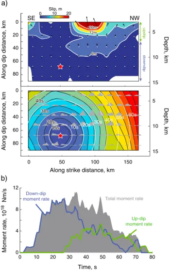
The preferred rupture model is displayed in Figure 4a. The rupture propagated primarily up dip and along strike toward the northwest, as found in earlier studies. The hypocenter is near the bottom edge of the model grid, which is seaward of the Mentawai Islands. This prevents the model from producing any significant vertical motion of the seafloor between the islands and mainland that would otherwise produce early arrival of a negative wave at Padang at odds with the observation. As demonstrated by Hill et al. [2012], deep slip on the megathrust close to the islands also produces strong GPS displacements, which are not desired given that the near-trench slip required by the tsunami observations is sufficient to account for the GPS signals. A high seismic moment patch is located over an area of ~80 km along strike and ~30 km along dip at depths from 7 to 10 km, with a maximum slip of ~8 m. The edge of this region is ~30 km from the hypocenter and begins to slip ~15 s after the rupture initiation. A shallower region of moderate
0 50 100 150 0 20 40 60 80 10s 20s 30s 40s 50s 60s 5 10 15 0 20 40 60 80 5 10 15
Along dip distance, km
Along dip distance, km
Along strike distance, km
Depth, k m Depth, k m SE 0 10 20 NW Slip, m 0 10 20 30 40 50 60 70 80 0 4 8 12 Time, s M oment rate , 10 18 N
m/s moment rateDown-dip Total moment rate
Up-dip moment rate
a)
b)
Figure 4. (a) Rupture plane views of the slip distribution for the pre-ferred model with a rupture velocity of 1.8 km/s. Slip is shown in the top and subfault source time functions in the bottom. The absolute depths of the nodes are shown on the right. The maximum slip of ~23 m occurs near the trench. Another near-trench rupture patch locates ~45 km farther to the northwest along the trench. A patch with maximum slip of 8 m locates from 7 to 10 km deep northwest of the
epicenter. The total seismic moment is 7.2 × 10²⁰N m (Mw7.8). The
hypocenter is marked with a redfilled star. The average slip direction at
each node is indicated with black arrows. The updip and downdip rupture area designations are assigned to the top two rows and the rest of the rows, respectively. Source time functions of each subfault node
are shown as grayfilled polygons. The centroid time of each node is
contoured as the background colored map. Constant rupture velocity expansion time counters are marked as white concentric circles. (b) The
overall source time function is shown as a grayfilled polygon. The updip
and downdip rupture source time functions are plotted with green and blue curves, respectively. The duration of each subfault source time
seismic moment but large slip ruptures the shallowest part of the model at depths less than 5 km near the trench, extending ~100 km along strike. This has a localized high-slip subregion about 45 km long with a maximum slip of ~23 m updip of the main seismic moment patch and a secondary peak of slip about 45 km farther to the northwest. The shallow sliding extends about 7.5 km seaward of the deformation front, but the precise upper limit of slip below the sediments is not resolved by the data, and it could be limited to the deformation front, which is along the grid points in thefirst row of the model. The shallow slip to the southeast in the model is also not spatially resolved by the data and may be an artifact.
The seismic moment associated with the central slip patch (38% of the total moment) is larger than that of the shallower slip patch (24% of the total moment). However, the estimated slip for the updip patch is significantly larger due to the lower shear modulus of the shallow layers in the velocity model. The shallow shear velocity in thefinal source model structure ranges from 1.7 km/s at the ocean bottom to 2.3 km/s at 6 km depth, and the rigidity is inferred from these low velocities. We lowered the very shallow sediment velocities somewhat from those imaged by Collings et al. [2012] (~2.5 km/s) to allow slip to increase to match the local tsunami amplitudes for the moment estimated from the inversion stage. This enhancement of slip is compatible with the seismic and geodetic data but is most directly driven by the matching of the tsunami signal from the nearby GPS buoy, as described below. There is poor resolution of the peak slip as it depends on the model discretization and rupture velocity, but the basic feature of patchy near-trench large slip is supported by the tsunami data. Individual subfault source time functions tend to be relatively smooth and triangular or trapezoidal in shape, lacking sharp peaks. This is controlled primarily by the relatively smooth teleseismic P wave signals. The total source duration continues for about 80 s, with the northwestern limit of the rupture being bounded by the location of the GPS buoy, which does not appear to directly overlie significant seafloor displacement.
We designate the shallowest two rows of the model grid as the updip fault portion and the deeper four rows as the downdip portion (Figure 4a). The moment rate functions for the separate updip and downdip portions are shown in Figure 4b. Overall, the downdip region has ~70% of the total seismic moment, while the updip region has ~30% of the total moment release. The moment rate during thefirst 25 s is dominated by the downdip region. This region reaches its peak moment rate around 20 s then decreases steadily to about 60 s with a broad triangular source function overall. The updip moment rate begins around 25 s, with a ramping increase that plateaus for ~45 s. These depth-varying contributions to the total moment rate function suggest a two-stage energy release that affects the observed waveforms.
3.2. Finite-Fault Model Predictions
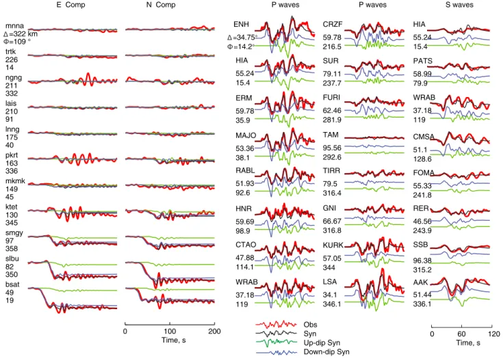
Teleseismic P and SH waves at northern stations show two dominant cycles beginning at 0 and ~40 s (Figure 5). These are mainly matched by the deeper and shallower slip patches, respectively, as shown by the separate model calculations displayed below the total waveform comparisons. This pattern of slip is compatible with the teleseismic body wave inversion shown by Lay et al. [2011b], which also had two distinct slip patches along dip. The shallow large slip patch is compatible with the constrained slip inversions of Hill et al. [2012], which were parameterized to concentrate slip updip with smooth decrease along dip. It is unclear whether there is any distinct spectral radiation character for the two regions, as the short-period P wave backprojections shown by Lay et al. [2011b] do not resolve the along-dip placement of coherent bursts of short-period radiation. The average teleseismic source spectrum shown by Lay et al. [2011b] further suggests some compound source structure, with indications of spectral corner frequencies near 0.05 Hz and 0.2 Hz that reflect the observed ground displacement character of several lower frequency oscillations with superimposed short-period oscillations apparent in Figure 5. The preferred model captures this quite well for thefinal, balanced weighting of the seismic and geodetic data sets in the joint inversion. The joint model accounts for 74% of the observed P and SH signal power, whereas separate inversions of just the seismic data account for about 78%. Comparison of all of the observed and synthetic body waves is shown in Figure S1. The model comparisons with the hr-GPS data (Figures 5 and 6) show good prediction of the timing of the rise time and total static offsets of the closer stations, with some, but not all of the later short-period oscillations being accounted for. The joint inversion underpredicts some of the localized short-period oscillations, but even separate inversion of just the hr-GPS signals does not provide significantly improved fits to the time-varying features at stations to the north (NGNG, PKRT, and KTET). We attribute these to either deficiencies of the local 1-D velocity model used to compute the time-varying Green functions, errors in estimating the
short-period hr-GPS ground motions, or our kinematic model intrinsically not accounting for off-fault local low seismic moment-triggered aftershocks along the northwestern direction. We explored the timing and possible moveout of some of the small features without successfully isolating any small subevents with negligible static contributions but sufficient surface wave excitation to match the features better than the average joint model. Decomposition of the hr-GPS signal predictions into contributions from the updip and downdip regions of the fault indicates different relative contributions compared with the teleseismic data set, as apparent in Figure 5. The static offsets at the hr-GPS stations (Figure 6 shows the observed and predicted values in map view) are mainly accounted for by slip in the downdip region (recognizing that all slip in this model is shallow in an absolute sense). The updip region produces minor Figure 6. Observed (red) and computed (black) static horizontal
dis-placements for 11 hr-GPS stations. Stations locations are marked with green triangles with station names. The rupture pattern of the preferred model is plotted with gray scale color. The trench location is marked with a barbed gray curve.
bsat slbu smgy ktet mkmk pkrt lnng lais ngng trtk mnna 49 19 82 350 97 358 130 345 149 45 163 336 175 40 210 91 211 332 226 14 =322 km =109 °
E Comp P waves P waves S waves
0 100 200 Time, s N Comp 0 60 120 Time, s ENH =34.75° =14.2° HIA 55.24 15.4 ERM 59.78 35.9 MAJO 53.36 38.1 RABL 51.93 92.6 HNR 59.69 98.9 CTAO 47.88 114.1 WRAB 37.18 119 CRZF 59.78 216.5 SUR 79.11 237.7 FURI 62.46 281.9 TAM 95.56 292.6 TIRR 79.5 316.4 GNI 66.67 316.8 KURK 57.05 344 LSA 34.1 346.1 HIA 55.24 15.4 PATS 58.99 79.9 WRAB 37.18 119 CMSA 51.1 128.6 FOMA 55.33 241.8 RER 46.56 243.9 SSB 96.38 315.2 AAK 51.44 336.1 Obs Syn Up-dip Syn Down-dip Syn
Figure 5. Observed (red) and modeled (black) ground displacement signals for hr-GPS and selected teleseismic P waves and S waves for the preferred joint inversion. The contributions to the total motion from updip and downdip regions of the model (Figure 4) are plotted with green and blue curves, respectively. Only horizontal components of the hr-GPS records are shown, ordered by epicentral distance. Teleseismic records are ordered by azimuth.
static displacements and seismic oscillations. This is controlled by the relative amplitude decay with distance of static and time-varying displacements and corresponds to the modeling nonuniqueness of the GPS static offsets discussed by Hill et al. [2012]. What differs most for our model is that we are inverting the full time-dependent motions in the hr-GPS records, with the timing of the ramping displacements and superimposed oscillations from body and surface arrivals helping to constrain the distance to the slip that accounts for the overall static offsets shown in Figures 5 and 6.
We performed separate inversions of just the hr-GPS signals, isolating the time varying and static motions, to evaluate the added spatial resolution provided by the former (Figure S2). This was done by computing ground velocity signals from the displacement records to isolate the dynamic part of the regional wavefield; we measure the static displacements from the hr-GPS data at times after all dynamic waves have passed. The same operations are applied to the Green functions, with separate nonnegative inversions of the velocity records and static displacements. Wefind that the main moment release patch is spatially resolved by the dynamic ground velocities and that some slip near the trench is consistently found in the inversions for various spatial smoothing factors. However, for inversions of the static ground displacements, no slip is resolved near the trench when using low spatial smoothing factors and very shallow slip only appears when heavy spatial smoothing is applied (Figure S2). We also performed inversions in which we removed the shallowest model row,finding stable features in the ground velocity inversions over the deeper model grid, but residual waveform misfit increases by 13%, due to inability of deeper slip to match timing of some motions. We found<1% misfit increase for the static inversions with the truncated model grid, indicating that deeper slip could compensate fully for the lack of very shallow model grid. These results indicate that the shallowest model row parameters are in the null space for the static displacement information, as noted by Hill et al. [2012] but do contribute to the time-varying signals somewhat. The time-varying features of the hr-GPS data thus provide improved absolute resolution of the slip in the deeper part of the model along with limited resolution of near trench slip due to timing of seismic wave arrivals, as found for previous inversions of hr-GPS data for offshore megathrust ruptures [e.g., Yue and Lay, 2011].
3.3. Tsunami Model Predictions
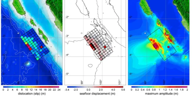
The iterative tsunami modeling adds critical resolution of the very shallow slip in ourfinite-fault model, primarily associated with the waveform at the nearby GPS buoy. The time-dependent seafloor deformation drives the tsunami model that in turn describes the evolution of the ocean waves around the landform and across the ocean. Figure 7 shows the fault slip distribution, total seafloor uplift and subsidence, and maximum tsunami wave amplitude for ourfinal model. The seafloor displacement pattern directly reflects the fault slip characteristics. The updip slip patch results in an elongated region of 1 to 2 m uplift and minor subsidence toward the Mentawai Islands. The updip slip gives rise to near-trench uplift of 5 m over an elongated patch and 1–2 m toward the northwest adjacent to the GPS buoy. The effects of seafloor motions arefiltered by dispersion before reaching the water surface. The elongated downdip and updip patches produce 1.4 and 2.9 m of tsunami wave amplitude, while the near-trench uplift patches in the northwest rupture region produces distinct waves of ~1.8 m amplitude. The tsunami waves are amplified over the shelves fronting the Mentawai Islands and focused in an offshore direction normal to the trench.
The excitation from these seafloor motions shapes the tsunami signals in the buoy and tide gauge recordings that are essential to the iterative modeling approach. Figure 8 illustrates the evolution of the near- and far-field tsunamis in relation to the seafloor motions (see Animations S1 and S2 for full sequence of the event). When the rupture stops at 0:01:20 (h:min:s), the long-crested waves generated by uplift along the trench and the elongated downdip slip patch have already begun to propagate away from the source. Diffraction at the crest termini results in two oblong systems of waves that are modulated by radiation from isolated slip patches over the rupture area. The radiated waves from the two near-trench uplift patches, superposed on the diffracted waves from the elongated patch along the trench, reach the GPS buoy at 0:04:30 and 0:07:00. The offshore component of the tsunami is dominated by the long-crested wave from the trench; the wave from the downdip patch diminishes through reverse shoaling as it propagates into deeper water. The two onshore waves shoal over the continental slope and merge into a single wave over the shelf, exacerbating the impacts to the Mentawai Islands. The snapshots at 0:30:00 and 0:45:00 show the wavefield between the islands and mainland is defined by diffraction through the channels between the Mentawai Islands. The offshore wavefield is dominated by a distinct crest generated at the trench followed by
Figure 8. Snapshots from Animations S1 and S2 showing evolution of the tsunami. The near-field tsunami consists of two oblong wave systems generated by the elongated, updip, and downdip slip patches. Onshore waves from the two patches merge over the continental shelf exacerbating the impacts to the Mentawai Islands. The offshore
waves from the downdip patch attenuate rapidly over the continental slope due to reverse shoaling. The far-field tsunami is dominated by the updip slip.
Figure 7. Map of the (left) fault slip, (middle) rock surface displacement, and (right) maximum tsunami wave amplitude for the rupture model of the 25 October 2010 Mentawai earthquake obtained by iterative modeling of hr-GPS, teleseismic P and S waves, and tsunami records. In Figure 7 (left), gray solid lines indicate depth contours at 1000 m intervals. In Figure 7 (middle), solid lines indicate uplift contours at 0.5 m intervals and dashed lines indicate subsidence contours at 0.2 m contours. White circles indicate water-level stations and red circles indicate the epicenter.
radiated waves from oscillations of the tsunami source and leakage of standing edge waves on the continental margin. The initial wave crest reaches Cocos Island at 1:18:00 and the DART buoy at 2:06:00. The wavefield shows significant scattering around Cocos Island due to diffraction of the tsunami waves and resonance oscillations in the island group.
Comparisons of observed and computed tsunami signals for thefinal model are shown in Figure 9. The computed spectra are based on 6 h of data from the earthquake initiation time and the results from the GPS buoy are omitted due to the short duration. The initial positive wave with double peaks at the GPS buoy is accounted for primarily by the variable slip along the shallowest row in the model. The two regions of localized seafloor uplift nearest to the buoy produce the double peaks, while the diffracted wave from the elongated, large slip patch accounts for the pulse in the background. Matching the timing of the two peaks places tight constraint on the along-strike location of the slip, which gave resolution of the rupture velocity of 1.8 ± 0.1 km/s for thefinal grid spacing. This sensitivity is due to the location of the buoy along the rupture direction, and Satake et al. [2013] similarly noted that this one observation strongly influenced the placement of shallow slip in their tsunami inversion. The early arrival of the second wave with multiple peaks points to a downdip slip patch that is closer to the epicenter than what is predicted by the present model.
The tsunami signals at the Padang and Cocos Island tide gauges and DART 56001 are matched reasonably well by the preferred model computations for over an hour after arrival and across the frequency range of interest. The computed tsunami at Padang is about 2 min late but has very similar waveform to the recording. A time shift aligns the signals for comparison. As apparent in Figure 8 and Animation S1, the tsunami signal at Padang results from superposition of diffracted waves around the Mentawai Islands through shallow passages. We explored extensions of the model grid farther northwest,finding that with slip extending as far as the GPS buoy, the timing could match the Padang records, but this produced strong arrivals not matching the signal at the GPS buoy. The overall Padang signal is not sensitive to the location and strength of very Figure 9. Comparison of observed (black) and computed (red) sea surface elevation (left) time series and (right) spectra for the 25 October 2010 Mentawai earthquake tsunami. The location of water-level stations is shown in Figure 2. The
computed series at Padang and Cocos Islands have been shifted by 2 and 4 min to align with the recorded signals.
The computed spectra are based on 6 h of data from the earthquake initiation time and the results from the GPS buoy are omitted due to the short duration.
shallow slip on the fault as the resulting wave merges with that from the downdip slip before reaching the Mentawai Basin. The signal reflects the overall slip distribution more than localized complexity. We did find that the region of downdip slip must have the spatial extent found in the preferred model to match the period of the signal at Padang. The arrival time error and subsequent dephasing might be attributed to the weakly dispersive properties of NEOWAVE that interfere with the nonlinear processes as the tsunami propagates from the Mentawai ridge into the Mentawai Basin through reverse shoaling [Bai and Cheung, 2013]. Small errors in the bathymetry can also accumulate travel time and phasing anomalies, even if the source model is accurate.
The waveformfit to the tide gauge signal at Cocos Island is very good after implementation of a 4 min time advance to the computed data. The agreement is greatly improved over the direct inversion results of Satake et al. [2013], apparently due to the detailed bathymetry of the atoll shown in Figure 2. We found from the iterative modeling approach that the signal is sensitive to the presence of strong slip at shallow depth in the model. This is due to the dominance of the tsunami waves from the shallow slip over those from the downdip patch as illustrated in Figure 8 and Animation S2. DART 56001 recorded weak diffracted waves in the strike direction. The signal reflects the spatial extent and magnitude of the rupture but does not resolve the localized pattern of heterogeneous slip. The agreement between the recorded and computed signals is very good in both amplitude and timing for over an hour after the main tsunami arrival (earlier short-period water oscillations from the main shock seismic waves are not modeled). Thefit to this signal is better than those achieved by the seismic models of Lay et al. [2011b] or Newman et al. [2011] and the geodetic model of Hill et al. [2012]. It is comparable to that of the tsunami inversion model by Satake et al. [2013].
Collectively, the various data sets add complementary constraints on thefinal rupture model. The combination of data types guides the convergence on a unified model that accounts for each data type almost as well as a separate inversionfit. While the diversity of data types compounds the difficulty of formally assessing error in the model parameters, we believe thefirst-order kinematics and slip pattern of our preferred model are a realistic source representation compatible with all of the data within reasonable limits of our confidence in the propagation effects.
3.4. Stress Drop and Shallow Slip Enhancement
Calculation of static stress drop for afinite-fault model with nonuniform slip is complex [e.g., Noda et al., 2013]. The area and slip distribution are affected by the model parameterization, smoothing, and intrinsic resolution of the model parameters, and it is necessary to adopt thresholds for defining the slip and area estimates. For the 2010 Mentawai earthquake, we constrain the area to that with significant slip spanning the fifth to eleventh columns along strike and the top four rows along dip. The average slip over this 7695 km2
area is ~6.5 m. The corresponding static stress drop estimate is 0.9 MPa, which is lower than the typical several MPa stress drop of interplate events. The estimated stress drop is similar to that for the 2006 Java tsunami earthquake (0.85 MPa) estimated fromfinite-fault model inversion [Ammon et al., 2006], twice the stress drop (~0.3 MPa) of the 1994 Java tsunami earthquake estimated from the source function spectrum corner frequency [Abercrombie et al., 2001], and 1 order of magnitude larger than estimated stress drop (<0.1 MPa) of 1992 Nicaragua earthquake [Velasco et al., 1994; Ye et al., 2013]. These four tsunami events all have low static stress drop<1 MPa, indicating this is a common feature for tsunami events.
The plate convergence rate normal to the trench direction is 45 mm/yr [Chlieh et al., 2008]. If we assume that strain accumulation all occurred since the great 1833 event in this region, with 100% locking, the accumulated slip deficit before 2010 was <8 m. Chlieh et al. [2008] estimate that the prism near the trench is ~ 40–50% locked, suggesting an ~4 m average slip deficit for a heterogeneously locked interface. While we believe there is very little resolution of near-trench locking, the estimated deficit is consistent with the average slip of the 2010 Mentawai event, so it is plausible that the event released much of the strain accumulated since 1833.
The localized peak slip near the trench (up to 23 m) is significantly higher than the post-1833 slip deficit (8 m). The peak slip value is not a stable feature infinite-fault model inversions, as it strongly depends on the smoothing factor used in our inversion. If the estimated peak slip value is correct, there may have been a patch that did not slip during the 1833 event, or there could be enhanced shallow slip during the dynamic rupture of 2010. Enhanced shallow slip near the trench occurred for the 2011 Tohoku event [Lay et al., 2011a;
Yue and Lay, 2011; Ito et al., 2011; Ide et al., 2011], with>60 m slip estimated near the trench in finite-fault model inversions and repeated bathymetry measurements, exceeding the ~20 m coseismic slip near the hypocenter in a region that had been 100% locked [Loveless and Meade, 2011]. For great megathrust events, dynamic overshoot of shallow slip may result from updip propagation of the rupture interacting with the free surface boundary condition, causing“fling” of the overlying wedge. For the 2010 Mentawai event, the rupture does appear to have propagated seaward, but only over modest rupture extent. Dynamical modeling is required to evaluate whether overshoot is involved in the enhanced slip in the localized patch.
4. Discussion
4.1. Differences From Previous Models
Our preferredfinite-fault model has similar overall northwestward directivity and faulting geometry, but larger slip near the trench than in previous models. Lay et al. [2011b] and Newman et al. [2011] analyzed teleseismic data sets,finding limited (~5 m) rupture extending to the trench. Hill et al. [2012] performed forward modeling of geodetic datafinding peak slip of ~12 m directly updip from the hypocenter. Satake et al. [2013] inverted tsunami observations with a coarse grid model,finding two near-trench rupture patches with slip of ~6.1 m and ~4 m each. Our modeling combines all of the data sets and alsofinds two shallow patches, but with larger slip than in the model of Satake et al. [2013]. Peak slip amplitude infinite-fault models is rarely well constrained, being strongly controlled by the regularization approach and reference velocity structure. The low shear velocity in our model near the toe scales up the shallow slip significantly, but there is substantial uncertainty in the precise structure. Our inversion regularization is selected by forward modeling of the tsunami signals. Tsunami waves, due to intrinsic low frequency content, are not sensitive to details of localized slip. Either slip over a small area, as ~20 m slip over 15 × 15 km2subfaults (as in our model), or more distributed slip over a larger area, such as ~6 m slip over 40 × 40 km2subfaults (as in Satake et al. [2013]), canfit the tsunami waves comparably well. Seismic potency, given by slip × area, in the vicinity of the peak slip in our model is compatible with that in Satake et al. [2013]. While not strongly resolved, we believe it is likely that slip>15 m occurred in a localized region. Near-trench deformation observations are needed to resolve the precise amount of slip.
The tsunami data confirm that the 2010 Mentawai tsunami earthquake has patchy shallow coseismic slip extending to near the toe of the accretionary prism. The plate interface near the trench is overlain by sediments with low rigidity, and this environment has often been assumed to be a low-seismicity area with slip velocity-strengthening friction that leads to stable sliding [e.g., Byrne et al., 1988; Scholz, 1988; Lay et al., 2012]. Neither of the preceding 2007 thrusting events ruptured up to the region that failed in 2010, as is commonly observed or at least believed to be the case for great interplate ruptures. Some great events, like the 2011 Tohoku earthquake, do have coseismic slip extending all the way to the trench, apparently driven by very large slip at greater depth, while large tsunami earthquakes like the 1896 Sanriku [Kanamori, 1972], 1992 Nicaragua [Kanamori and Kikuchi, 1993; Imamura et al., 1993; Velasco et al., 1994; Satake, 1994], 2006 Java [Ammon et al., 2006], and 2010 Mentawai rupture entirely within the shallow part of the trench. Tsunami events typically have long source durations, limited short-period energy radiation, and low energy/moment ratio [Polet and Kanamori, 2000; Lay and Bilek, 2007; Lay et al., 2012], and all of these characteristics are found for the 2010 Mentawai earthquake, along with the low static stress drop discussed above.
4.2. Pre-Event Seismicity and Fault Locking
Efforts to image the pre-2007 state of locking of the megathrust using SuGAr GPS observations and coral records [Chlieh et al., 2008] did not resolve strong locking far offshore in the vicinity of the 2010 rupture zone due to lack of resolution, with the 60% locking region being outlined by green dashes in Figure 10. The 2007 earthquakes produced moderate size aftershocks around the region that failed in 2010, but only one event is located within the 2010 coseismic slip zone, as indicated by the GCMT focal mechanisms shown in Figure 10. Many of these are interplate thrust mechanisms, but some are intraplate extensional or upper plate backthrust faulting. Most of the aftershocks locate along the margins of the large-slip zones for the 2007 event, but none extend into the shallowest megathrust region, consistent with presence of an updip seismic front. We calculate the coseismic Coulomb stress change caused by the 2007 Bengkulu and Pagai-Sipora events using thefinite-fault models obtained by Konca et al. [2008] and assuming a shallow thrust faulting
orientation as a target loading geometry. The results are shown in Figure 10a. Near Sipora Island, located in between large-slip areas of the 2007 events, there is a concentration of aftershocks highlighted in Figure 10b. This is a region with little Coulomb stress increase (<0.1 MPa) from the large events. The pre-2007 locking pattern shows a gap with reduced value near Sipora Island. This indicates a region with reduced strain accumulation that may have acted as a barrier to rupture expansion in the 2007 events but experienced accelerated post-event deformation.
A zone of afterslip has been reported downdip of the 2010 rupture zone [Lubis et al., 2013] for the interval within 15 months after the 2007 events, as indicated in Figure 10. The maximum afterslip amount was 0.5 m near the Pagai Islands, after poroelastic and viscoelastic deformation was removed. This afterslip region locates between the 2007 and 2010 coseismic rupture patches and the concentrated aftershock area, with few aftershocks within the region. This area may experience predominantly slow slip, with viscoelastic deformation or stable slip that could also have delimited the 2007 rupture extent. Afterslip may also have occurred updip of the Bengkulu rupture zone extending from the shallow aftershock activity to the trench (J.-P. Avouac and L. Tsang, personal communication, 2014), but the shallow region of the 2010 failure is likely to have remained fully locked, receiving progressive loading from the adjacent 2007 earthquakes, their afterslip, and their aftershocks.
Most of the 2007 events interplate thrust aftershocks are located within the driving stress increase surrounding the large-slip regions of the 2007 events. This increase overlaps the downdip edge of the 2010 rupture zone, consistent with stress loading near its hypocenter. The region northwestward from the 2007 events as far as the 1935 (MS7.7) rupture [Rivera et al., 2002] southeast of the 2005 Nias (Mw8.7) earthquake zone has presumably accumulated strain since 1797 [e.g., Chlieh et al., 2008; Nalbant et al., 2013].
4.3. The 2010 Event Aftershock Distribution
Larger aftershocks within 1 month after the 2010 Mentawai event with faulting solutions in the GCMT catalog mostly locate in the vicinity of the near-trench slip patch with normal fault focal mechanisms (Figure 11). Relocations of these events together with the GCMT depths suggest that the hypocentral depths are 10–20 km, placing these normal events in the subducting slab [Bilek et al., 2011]. Bending of the subducting plate as it approaches the trench causes shallow tensile stress normal to the trench direction that produces normal faults. These can be activated by Coulomb stress changes from the interplate thrusting. Significant normal faulting aftershocks have also been reported for previous tsunami events, notably the
Figure 10. Comparison of the 2010 slip model with prior event slip models, regional focal mechanisms, and estimates of prior slip deficits. In Figures 10a and 10b, the
coseismic slip areas of the 2007 Bengkulu and Kapalauan and 2010 Mentawai events are indicated with white contoured (2 m and 6 m), grayfilled patches. GCMT
foreshock and aftershock solutions are plotted in black and bluefilled focal mechanisms, respectively. (a) The Coulomb stress change produced by the 2007 events
on the megathrust geometry (cyanfilled mechanism) is mapped with a blue-red color map (legend) within the region of the cyan dashed lines. Foreshock and
aftershock (2007–2010) focal mechanisms are plotted with black and blue fill, respectively. (b) The 60% locked interseismic area preceding 2007 [Chlieh et al., 2008] is
outlined with green dashed line. An afterslip region [Lubis et al., 2013] is indicated with a transparent bluefilled patch. An area with concentrated seismic activity
1994 and 2006 Java tsunami earthquakes [El Hariri and Bilek, 2011]. We calculated the coseismic Coulomb stress change at 15 km depth on a target normal faulting focal mechanism (Figure 11a) andfind that most of the extensional activity locates within the zone with Coulomb stress increase of>1.0 MPa.
There were two early interplate thrust aftershocks downdip from the 2010 rupture, and subsequent activity over the next 3 years locates near the hypocenter and downdip edge of the 2010 Mentawai rupture. These events also appear to be confined to regions on the margins of the large-slip zone of the 2007 Bengkulu event. Calculated Coulomb stress change produced by the 2010 event for thrust events along the dipping megathrust (Figure 11b) also shows most events locating within regions of increased driving stress>1.0 MPa. Some regional activity is beyond the likely influence of the 2010 event and may represent continuing aftershocks of the 2007 ruptures or a return to background activity. The large slip, activation of surrounding extensional faulting, and lack of aftershock activity colocated with the coseismic slip suggest significant, if not total stress release on the megathrust region in the 2010 rupture zone [e.g., El Hariri and Bilek, 2011].
5. Conclusions
Using an iterative modeling strategy involving joint inversion of hr-GPS and teleseismic data sets and forward modeling of high-quality tsunami observations, we obtained a self-consistent coseismic rupture model for the 2010 Mentawai tsunami earthquake compatible with all three data sets. In our preferredfinite-fault model, coseismic slip reaches the toe of the accretionary prism with a localized zone of slip of up to ~23 m near the trench. The slip distribution involves initial rupture of a fault patch at depths from 7 to 10 km with an overall triangular source time function followed by shallower rupture along the trench at depths less than 5 km with a prolonged plateau-shaped source time function. A relatively low stress drop (0.9 MPa) is estimated for ourfinite-fault model, which is lower than typical thrusting events but consistent with previous tsunami earthquake stress drops. The large slip near the trench may present some dynamic enhancement of slip or possibly localized accumulation of strain that dates back to before the 1797 and 1833 ruptures. The rupture area of the 2010 Mentawai event is updip of the rupture zones of the 2007 Bengkulu and Pagai-Sipora events, and aftershock and afterslip zones of those events frame the downdip edge of the 2010 rupture. The regional megathrust has localized patches of strong or weak coupling that appear to be activated differently with afterslip or aftershock concentrations. There was little direct indication of locking of the 2010 rupture zone before or after the 2007 events, and there is no clear distinction relative to the uppermost megathrust regions to the southeast and northwest to guide the assessment of further tsunami earthquake activity in the region. The most important lesson from this earthquake is that it is not safe to Figure 11. Comparison of the 2010 slip model Coulomb stress changes on extensional and compressional faulting geometries near the rupture zone. In both panels, the coseismic rupture patches of the 2007 and 2010 main shocks are plotted as in Figure 10. The global centroid moment tensor best double couple mechanism for aftershocks within 1 month and from 1 month to 3 years after the 2010 Mentawai event is plotted with red and purple mechanisms, respectively. (a) The Coulomb stress change caused by the 2010 Mentawai event is projected to a normal fault geometry at 15 km depth and plotted with the blue-red scale. The focal mechanism of the receiver fault is shown. (b) Coseismic Coulomb stress change caused by the 2010 Mentawai event is projected to the fault geometry of the megathrust and plotted in a blue-red color scale. The receiver fault mechanism is indicated with a cyan focal mechanism. The color scale of both Coulomb stress maps is shown in the bottom left of Figure 11b.