HAL Id: hal-00298278
https://hal.archives-ouvertes.fr/hal-00298278
Submitted on 14 Nov 2005
HAL is a multi-disciplinary open access
archive for the deposit and dissemination of
sci-entific research documents, whether they are
pub-lished or not. The documents may come from
teaching and research institutions in France or
abroad, or from public or private research centers.
L’archive ouverte pluridisciplinaire HAL, est
destinée au dépôt et à la diffusion de documents
scientifiques de niveau recherche, publiés ou non,
émanant des établissements d’enseignement et de
recherche français ou étrangers, des laboratoires
publics ou privés.
ice-ocean system: the role of the thermal and
mechanical forcing
W. Lefebvre, H. Goosse
To cite this version:
W. Lefebvre, H. Goosse. Influence of the Southern Annular Mode on the sea ice-ocean system: the
role of the thermal and mechanical forcing. Ocean Science, European Geosciences Union, 2005, 1 (3),
pp.145-157. �hal-00298278�
SRef-ID: 1812-0792/os/2005-1-145 European Geosciences Union
Influence of the Southern Annular Mode on the sea ice-ocean
system: the role of the thermal and mechanical forcing
W. Lefebvre and H. Goosse
Universit´e Catholique de Louvain, Institut d’astronomie et de g´eophysique Georges Lemaˆıtre, Belgium Received: 2 June 2005 – Published in Ocean Science Discussions: 27 June 2005
Revised: 15 September 2005 – Accepted: 4 November 2005 – Published: 14 November 2005
Abstract. The global sea ice-ocean model ORCA2-LIM is
used to investigate the impact of the thermal and mechanical forcing associated with the Southern Annular Mode (SAM) on the Antarctic sea ice-ocean system. The model is driven by idealized forcings based on regressions between the wind stress and the air temperature at one hand and the SAM index the other hand. The wind-stress component strongly affects the overall patterns of the ocean circulation with a northward surface drift, a downwelling at about 45◦S and an upwelling in the vicinity of the Antarctic continent when the SAM is positive. On the other hand, the thermal forcing has a neg-ligible effect on the ocean currents. For sea ice, both the wind-stress (mechanical) and the air temperature (thermal) components have a significant impact. The mechanical part induces a decrease of the sea ice thickness close to the conti-nent and a sharp decrease of the mean sea ice thickness in the Weddell sector. In general, the sea ice area also diminishes, with a maximum decrease in the Weddell Sea. On the con-trary, the thermal part tends to increase the ice concentration in all sectors except in the Weddell Sea, where the ice area shrinks. This thermal effect is the strongest in autumn and in winter due to the larger temperature differences associated with the SAM during these seasons. The sum of the thermal and mechaninal effects gives a dipole response of sea ice to the SAM, with a decrease of the ice area in the Weddell Sea and around the Antarctic Peninsula and an increase in the Ross and Amundsen Seas during high SAM years. This is in good agreement with the observed response of the ice cover to the SAM.
1 Introduction
The Southern Annular Mode (SAM, also referred as the Antarctic Oscillation (AAO) or High Latitude Mode (HLM))
Correspondence to: W. Lefebvre
is the dominant mode of variability of the atmospheric circu-lation southwards of 20◦S. It is associated with changes in
the position and the strength of the westerlies (e.g. Connol-ley, 1997; Gong and Wang, 1999; Thompson and Wallace, 2000; Simmonds, 2003) that induce a stronger Ekman Drift towards the north in the Southern Ocean during years with high SAM index as well as an increased upwelling close to the continent and a downwelling around 45◦S (Mo, 2000; Watterson, 2000, 2001; Cai and Watterson, 2002; Hall and Visbeck, 2002; Lefebvre et al., 2004).
The influence of the SAM on the ice cover appears more complex (Kwok and Comiso, 2002; Liu et al., 2004; Lefeb-vre et al., 2004) than this annular oceanic response, whose main characteristics are similar at all the longitudes. Indeed, the correlation between the SAM index and the ice extent displays a dipole, with more ice in the Ross Sea and less in the Weddell Sea. This clearly non-annular pattern appears driven by a decrease in sea level pressure in the Amundsen-Bellingshausen Seas when the SAM is high. This induces a deflection of the westerlies towards the south-east around the Peninsula and towards the north-east in the Ross Sector. These winds change the sea ice velocities, the advection of heat by the ocean current and advect also warmer air in the Weddell Sea and colder air in the Ross Sea, resulting in the dipole described above (Lefebvre et al., 2004). Those studies also underline that in some regions, the SAM explains only a small fraction of the internal variability of the system and a lot of other factors must be invoked in order to understand the variability of the Southern Ocean.
The SAM has a distinct effect on the location and the strength of the Antarctic Circumpolar Current (ACC), al-though the lack of coherence between the SAM and the cir-cumpolar current on the multidecadal timescale shows that the circumpolar current is primarily controlled by another mode on long timescales (Hall and Visbeck, 2002). Further-more, antropoghenic factors, could influence both the ACC and the SAM, for instance by Fyfe and Saenko (2005).
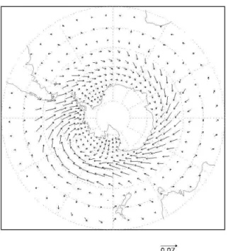
Fig. 1. Annual mean of the regression between the wind stress
(N
m2) and the annual mean SAM index for the period 1980–
1999. This pattern has been used in the idealized forcings M+, S+ (NCEP/NCAR wind stress forcing + regression), M− and S− (NCEP/NCAR wind stress forcing – regression).
The goal of this study is to provide further information about the origin of the response of the sea ice and the ocean to the SAM. In particular, we try to disentangle the effect of the wind stress change from those resulting from the changes in air temperature. To do so, several numerical experiments have been performed with the coupled sea ice-ocean model ORCA2-LIM (Timmermann et al., 2005). In those experi-ments, we force the model with idealized forcings derived from the regressions between the SAM and the air temper-ature and the wind stress, respectively. The model and the forcings are briefly described in Section 2. Section 3 pro-vides a justification of our methodology. In Sects. 4 and 5, the responses to the thermal and the mechanical forcing are analyzed. Finally, the conclusions are presented.
2 Model description and experimental design
2.1 Model description
The model used here, called ORCA2-LIM, results from the coupling of the Louvain-la-Neuve sea ice model (LIM) (Fichefet and Morales Maqueda, 1997) with the hydrostatic, primitive equation ocean model OPA (Oc´ean PArall´elis´e) (Madec et al., 1999). The coupling technique between OPA and LIM is identical to the one described in Goosse and Fichefet (1999). The model version used here is exactly the
same as the one that has been used in Lefebvre et al. (2004), which includes a more extensive model description.
OPA is a finite difference ocean general circulation model with a free surface and a non-linear equation of state in the Jackett and McDougall (1995) formulation. The thermody-namic part of LIM uses a three-layer model (one layer for snow and two layers for ice) for sensible heat storage and vertical heat conduction within snow and ice while the sea ice velocity field is determined from a momentum balance considering sea ice as a two-dimensional continuum in dy-namical interaction with atmosphere and ocean. The viscous-plastic constitutive law proposed by Hibler (1979) is used for computing internal stress within the ice for different states of deformation.
The coupled model is run on a global grid with 2◦nominal resolution and a mesh refinement in high latitudes and near the equator. As a consequence, the meridional resolution in-creases to 0.5◦close to the Antarctic continent, correspond-ing to a horizontal grid width of about 50 km. Vertical dis-cretization uses 30 z-levels, with 10 levels in the top 100 m. Model runs are initialized using data from the end of the 46-yr experiment described by Timmermann et al. (2005). Daily 2-m air temperatures and 10-m winds from the NCEP/NCAR reanalysis project for the period 1980–1999 (Kalnay et al., 1996), and monthly climatologies of surface relative humid-ity (Trenberth et al., 1989), cloud fraction (Berliand and Strokina, 1980), and precipitation rate (Xie and Arkin, 1996) are utilized to drive the model. The surface fluxes of heat and moisture are determined from these data by using empirical parameterizations described by Goosse (1997).
A correction of ocean surface freshwater fluxes has been derived from the time-mean restoring salinity flux diagnosed from the experiment described by Timmermann et al. (2005) in order to circumvent the surface salinity drift that occurs through the lack of any stabilizing feedback if the model is forced with slightly incorrect evaporation, precipitation and/or river runoff fields.
2.2 Experimental design
In addition to the control run (CTRL) analyzed in Lefebvre et al. (2004), a series of experiments has been performed in which a perturbation of the forcing is applied on top of the normal forcing. Those idealized perturbations are derived from the regression between the SAM-index (defined as the leading principal component and the monthly NCEP reanal-ysis (Kalnay et al., 1996) sea level pressure anomalies south of 20◦S, which can be found at http://www.jisao.washington.
edu/aao/slp/) with the wind stress and the air temperature for the period 1980–1999. In a first group of experiments (me-chanical forcing), the perturbation is applied only to the wind stress: in M+, an annual anomaly of the wind stress corre-sponding to one standard deviation of the SAM (regression pattern of Fig. 1) is added, while this anomaly is substracted in M− (Table 1). In a second group of experiments, the
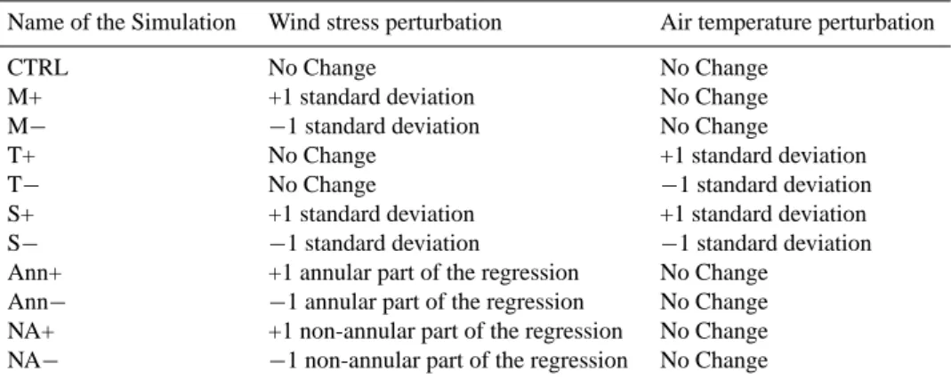
Table 1. Description of the experiments.
Name of the Simulation Wind stress perturbation Air temperature perturbation
CTRL No Change No Change
M+ +1 standard deviation No Change M− −1 standard deviation No Change
T+ No Change +1 standard deviation T− No Change −1 standard deviation S+ +1 standard deviation +1 standard deviation S− −1 standard deviation −1 standard deviation Ann+ +1 annular part of the regression No Change
Ann− −1 annular part of the regression No Change NA+ +1 non-annular part of the regression No Change NA− −1 non-annular part of the regression No Change
perturbation is only applied to the air temperature: in T+, a seasonal anomaly of the air temperature corresponding to one standard deviation of the SAM (regression patterns found in Fig. 2) is added, while this anomaly is substracted in T−. In a third group of experiments, both the air temperature and the wind stress forcing have been perturbed. Adding to the standard forcing one regression between the wind stress and the air temperature and the SAM, results in S+. Subtracting them gives S−. All these forcings have been imposed dur-ing the period 1980–1999 (see also Sect. 3). Nevertheless, as discussed in Sect. 3, we will use below only the first seven years of the simulation. This provides a robust description of the model response to the idealized forcing while avoiding some long-term effects that are not the subject of the present study.
The mechanical forcing (Fig. 1) displays an almost annu-lar signal, with wind stress anomalies coming from the north-west. However, in the Weddell Sea and around the Antarc-tic Peninsula, the northern component is more intense. In Ross Sea the wind stress anomaly is in general eastwards between 50◦S and 60◦S and directed northwards close to the continent. Those regional features are due to the SAM-related low-pressure area in the Amundsen-Bellingshausen Seas (Limpusavan and Hartmann, 2000). Furthermore, the increase in the magnitude of the westerlies associated with a high SAM index is slightly stronger in the Ross and Amund-sen Sectors than in the Weddell and Indian Sectors.
In order to compare the impact of the annular component of the wind stress anomalies with the non-annular part, due to the low pressure in the Amundsen-Bellingshausen Seas, an additional series of experiments has been performed (Ta-ble 1). In a first group of experiments, only the zonal mean of the wind stress regression is applied (annular part of the forcing): in Ann+, the zonal mean is added to the standard forcing for the years 1980–1999, while the anomaly is sub-stracted in Ann−. In a last series of experiments, the same methodology has been used for the non-annular anomalies
(NA+ and NA−) obtained by subtracting the zonal mean from the wind stress pattern of Fig. 1.
In all seasons, the air temperature above the Weddell Sea and around the Antarctic Peninsula is higher when the SAM is positive, while everywhere else the air temperature is lower, especially close to the continent (Fig. 2). This is in good agreement with the regression data from Thompson and Solomon (2002), who saw the same pattern in the air tem-perature data series on the Antarctic continent. The biggest changes are observed in autumn and winter. Although these air temperature changes appear quite large, the correlation is low (at maximum around 0.4) (Lefebvre et al., 2004). This is related to big natural variations in air temperature in this region and thus a large standard deviation of the air temper-ature there that leads to large regression values despite those low correlations. This implies that, even if we find a robust response of the ocean on the air temperature forcing, the low correlations of the SAM with the air temperature warns us that a lot of other factors will be at least as important for temperature changes as the SAM. As the air temperature re-gression pattern to the SAM is clearly non-annular, analyzing the influence of the zonal mean changes in a way similar to experiments Ann and NA for the air temperature forcing ap-pears not very instructive and such experiments are not dis-cussed here.
The method presented here has the advantage that we keep the interannual variability of the forcing (as we keep on hav-ing the variability in the NCEP-NCAR dataset) and that we can identify clearly the role of each component of the atmo-spheric forcing (wind stress or air temperature). However, this method can only be successful if the linearization pro-vides a good approximation of the response of the real system and if there are no big, either positive or negative, feedbacks between the oceanic response on the wind stress on the one hand and the air temperature on the other hand. Furthermore, the method could pose problems because the same perturba-tion is applied every year. After a few years, the long term
Fig. 2. Seasonal mean of the regression between the air temperature (◦C) (NCEP-NCAR reanalysis (Kalnay et al., 1996)) and the seasonal mean SAM index (NCEP-NCAR reanalysis) for the period 1980–1999. (a) summer, (b) autumn, (c) winter, and (d) spring. Contour interval is 0.3◦C. Solid lines correspond to positive values, while dotted lines show negative values. Shading in dark gray means a regression of more than 1◦C, whereas shading in light gray shows a regression of less than −1◦C. This pattern has been used in the idealized experiments T+, S+ (NCEP/NCAR air temperature forcing + regression), T− and S− (NCEP/NCAR air temperature forcing – regression).
response of the system to a constant perturbation could thus be different than the one observed in the real world where the polarity of the SAM changes nearly each year. These limitations will be discussed in Sect. 3.
3 Justification of the experimental design
3.1 Checking the linearity and comparing with the obser-vations
The approach of this paper is only valid if the southern sea ice-ocean system responds approximately in a linear way to the SAM. This assumption could be decomposed in two parts. Firstly, it is necessary to check that the sum of the
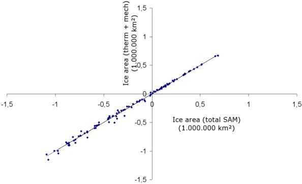
Fig. 3. For the first seven years of the simulations (15 points per year), we represent the following sums: on the X-axis; the ice area (in
1 000 000 km2) of (‘S+’ − ‘S−’)/2 and on the Y-axis; the ice area (in 1 000 000 km2) of (‘M+’ − ‘M−’ + ‘T+’ − ‘T−’)/2. The line (X=Y) shows a perfect correspondence between the different sets of experiments.
response to the thermal forcing only and to the mechanical forcing only is equal to the response to the total forcing and that this response is comparable to the results of the control experiment (Lefebvre et al., 2004) and to the observations. To illustrate that, we have displayed on Fig. 3 the sum of the response of the total sea-ice area to the thermal and mechan-ical forcing taken separately (y-axis) as a function of the sea ice area response to the total (thermal + mechanical) forc-ing (x-axis). For each dot, we have selected the same time during the first seven years of the experiments in all exper-iments in order to have a reasonable sampling of simulated variability. As can be seen, the correlation is very good, so we can state that if we are able to understand the response to the individual forcings, we also understand the response to the total idealized forcing associated to the SAM. Further-more, it is necessary to check if the response to this ideal-ized forcing (S) is similar to the observed response of the ice cover to the SAM. The validity of this hypothesis is shown clearly on Fig. 4. We see that the geographical distribution of the winter sea ice response to the idealized SAM forc-ing in the model is very similar to the observed response in the HadISST-dataset (Rayner et al., 2003). As discussed in Lefebvre et al. (2004), this observed response is also very close to the one obtained in the control experiment. Nev-ertheless, there are some discrepancies that must be kept in mind when interpreting the model response, in particular, the model tends to underestimate the decrease in sea ice concen-tration in the Amundsen-Bellingshausen Sectors associated with a positive SAM index, while the decrease is overesti-mated in the Weddell Sector.
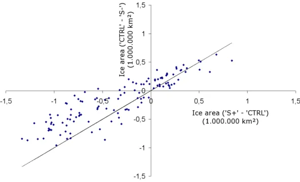
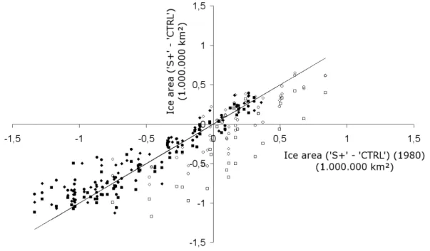
As a second aspect of the linearity issue, one has to de-termine if the response to an upward change in the SAM is the opposite of the response to a similar downward change in the SAM. As can be seen on Fig. 5, this is not totally valid. There is a clear linear relationship between the response to positive and negative anomalies. But, the changes induced by a decrease in the SAM are smaller than the responses due to an increase in the SAM. More precisely, on Fig. 6, we ob-serve that the spatial distribution of the anomalies is similar in experiments S+ and S− but the magnitude of the changes is larger is S+.
3.2 Checking the dependency of the results to initial condi-tions and the long term effect of the SAM
The response to the SAM could be influenced by the choice of initial conditions and by the years selected to start the ex-periments. For example, if the SAM is already high during the first year of the experiment, does an increase of the SAM has the same effect as if the SAM was initially low? If the initial state was a cold one with a lot of sea ice, will this in-fluence the response of the sea ice to the SAM? To answer these questions, we have started the idealized simulations at different years. In the standard experiment, the simulations are started in 1980. In addition, we have carried out experi-ments similar to S+ but starting in 1981, 1982 and 1983. For each of those experiments, the model is initialised using the corresponding year of the control run. The anomalies due to the modified forcings have been compared to the perturba-tions obtained for the experiments starting in the year 1980.
Fig. 4. (a) Half of the differences in sea ice concentration at the end of July between S+ and S− for the first seven years of the idealized
simulations. (b) Regression between the seasonal mean SAM index and the July mean ice concentration for the period 1980–1999 in the HadISST1 Rayner et al. (2003) observations. Contour interval is 0.05. Solid lines are positive values, while dotted lines show negative values. Shading in dark gray means a value of more than 0.1, whereas shading in light gray shows a value of less than 0.1.
Fig. 5. For the first seven years of the simulations (15 points per year), we represent the following sums: on the X-axis; the ice area (in
1 000 000 km2) of (‘S+’ − ‘CTRL’) and on the Y-axis, the ice area (in 1 000 000 km2) of (‘CTRL’ − ‘S−’). The line (X=Y) shows a perfect correspondence between the different sets of experiments.
We can see that the results of the various experiments (Fig. 7) are, in general, similar, although all the simulations starting in 1981, 1982 and 1983 seem to have slightly less ice the
standard experiment. More precisely, they show a stronger response of the sea ice area if the sea ice area anomaly is negative and a smaller response if this anomaly is positive. If
Fig. 6. (a) The difference in sea ice concentration at the end of July between S+ and CTRL for the first seven years of the idealized
simulations. (b) The difference in sea ice concentration at the end of July between S− and CTRL for the first seven years of the idealized simulations. Contour interval is 0.05. Solid lines are positive values, while dotted lines show negative values. Shading in dark gray means a value of more than 0.1, whereas shading in light gray shows a value of less than 0.1.
Fig. 7. The dependency of the sea ice response to the SAM to the initial conditions. Each point represents a comparison between two different
initial conditions at a certain time after starting the experiment with S+ forcing. On the x-axis: the sea ice area anomaly (in 1 000 000 km2) (difference with the CTRL-run) after a certain time after the starting of the simulation in 1980. On the y-axis: the sea ice area anomaly (in 1 000 000 km2) (difference with the CTRL-run) after a certain amount of time after the starting of the simulation in 1981 (diamonds), in 1982 (squares) and in 1983 (circles). If the time after the beginning of the simulation is smaller than two years empty symbols are used, otherwise filled symbols are used. The line shows the perfect correspondence, i.e. the case where we get exactly the same differences whatever year we take.
Fig. 8. Half of the differences in sea ice concentration at the end
of July between T+ and T− for the first seven years of the ideal-ized simulations. Contour interval is 0.05. Solid lines are positive values, while dotted lines show negative values. Shading in dark gray means a value of more than 0.1, whereas shading in light gray shows a value of less than 0.1.
we split up the results in two parts: on the one hand, the first two years after the beginning of the perturbation (empty sym-bols) and on the other hand, the other years (full symsym-bols). We see that the initial conditions only play a role in the first years of the idealized simulations. Even in these years, the differences (memory effect) in the changes of the sea ice area due to the SAM, in general, account for about 200 000 km2 only. This shows that the influence of initial conditions and starting years is weak. In addition, as the difference in the response of the runs starting in different years decrease with time, the observed trend in the SAM has only a negligible effect on our results. Furthermore, the natural trend of the SAM showed a sharp jump upwards at the end of the sev-enties. Afterwards, the index shows a sharp decline and a slight upwards trend (Marshall, 2003). In our results of the runs starting in different years, we do not see a difference that could be attributed to these natural changes in the trend of the SAM index.
Finally, we have to take into account another possible problem. We are using, in the different runs, a constant per-turbation year after year. As a consequence, long term effects could kick in after a few years. The first signal of such a long term effect can be seen after eight years, when an increased convection around Maud Rise can be found in the M+ and the S+ experiments. To eliminate these unwanted effects, we will work in the rest of this paper with means over the first seven years of the simulation. The sea ice response to the SAM in
these years, does not differ a lot from one year to another, so by averaging over these years, a reasonable SAM-like sea ice response is obtained (see above). The period 1980–1986 of the simulation provides thus a good representation of the subdecadal model response associated to the idealized per-turbation. As a consequence, only results for this period are presented here. Nevertheless, analysing a period of similar length but starting at a different date would give similar con-clusions.
The discussion presented in this section illustrates that the linear hypothesis used to construct our experimental design is reasonable. Our numerical experiments could thus be used to better understand the response of the ocean and sea ice as discussed hereafter.
4 Role of the thermal forcing
The response of the Southern Ocean to the thermal part of the SAM is relatively straightforward. The colder air in the Indian, Pacific, Ross and Amundsen sectors induces a larger sea ice cover in these regions (Figs. 2 and 8). The effect is the strongest during the seasons with the biggest changes in temperature: autumn and winter. However, in the the Wed-dell and Bellingshausen sectors, an increase in air tempera-ture results only in a marginal decrease in winter sea ice con-centration (see Fig. 8). The autumn ice production is lower in these regions due to the large temperature differences in this season (Fig. 2) inducing a lower ice extent (not shown). The difference in temperature decreases strongly in the win-ter and this induces only a small effect on the winwin-ter sea ice cover, as shown in Fig. 8. We have also to take into account the discrepancies between the observations and the model in this region, as mentioned in Sect. 3.1.
The net effect of the thermal forcing is an increase in sea ice area associated with a positive SAM index (Ta-ble 2), which reaches its maximum in June with a value of 538 000 km2. The change in air temperature does not have, as could be expected, much effect on the currents. Further-more, there are no big changes in the mixed layer depth in response to the changes in air temperature, even when taking into account the sea ice changes. However, we must recall here that the forcing used in our simulation does not include any interannual variation in precipitation and features only a reduced variability of surface heat fluxes (only temperature is varying). Taking into account this additional variability might alter the conclusion about the effect of the SAM on the density flux (e.g. Genthon et al., 2003).
5 Role of the mechanical forcing
In contrast to the thermal part, the mechanical forcing im-plies complex mechanisms. When the SAM index is high, the stronger westerlies induce enhanced zonal ocean surface currents and, due to the Ekman drift, also stronger meridional
Table 2. Ice area winter (JAS) differences between the different simulations in 1 000 000 km2. T: (‘T+’ – ‘T−’)/2. M: (‘M+’ – ‘M−’)/2. Ann: (‘Ann+’ – ‘Ann−’)/2. NA: (‘NA+’ – ‘NA−’)/2. S: (‘S+’ – ‘S−’)/2. The division into sectors is as follows: Weddell Sea (60◦W– 20◦E), Indian Ocean (20◦E–90◦E), Pacific Ocean (90◦E–160◦E), Ross Sea (160◦E–140◦W) and the Amundsen-Bellingshausen Seas (140◦W–60◦W).
Weddell Indian Pacific Ross Amundsen- Total Bellingshausen T −0.035 0.136 0.117 0.091 0.030 0.339 M −0.326 −0.118 −0.071 0.035 −0.051 −0.530 Ann −0.219 −0.089 −0.029 −0.015 −0.052 −0.403 NA 0.058 0.098 0.029 0.078 0.015 0.279 S −0.382 −0.020 0.034 0.110 −0.010 −0.269
currents (Fig. 9). This is the source of a horizontal divergence close to the Antarctic continent (around 65◦S), which leads to oceanic upwelling there. A horizontal convergence can be found at 45◦S and, as a consequence, a downwelling oc-curs there. The anomalous vertical velocities have the same sign over the whole depth of the Southern Ocean. On the other hand, the northward surface current is balanced by a southward flow around 2300 m depth (not shown). All these results are in fine agreement with the results of Hall and Vis-beck (2002) and Oke and England (2004). In the latter paper, the oceanic response to a change in the latitude of the South-ern Hemisphere Subpolar Westerly Winds was investigated, which is closely related to the SAM. In our simulations, the enhanced zonal currents give a relatively small increase in the Antarctic Circumpolar Current but its location does not change. These results are also in agreement with Hall and Visbeck (2002).
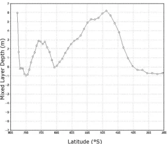
The annual mean of the zonal mean response of the mixed layer depth is displayed in Fig. 10. We can see an increase of the mixed layer depth in the Southern Ocean at almost all latitudes with a peak between 45◦S and 60◦S. This increase is likely due to wind stirring as the region between 45◦S and 60◦S is also the region where the largest changes in wind stress occur. Because of the time average, Fig. 10 hides also the differences between the seasons. In particular, during the local summer, the changes are generally of the order of a few meters, but in winter they reach locally 80 m. Although the wind stirring plays the dominant role on the zonal mean, the changes in the vertical velocity could also affect the stability of the water column locally and thus have an influence on the mixed layer depth, as discussed below.
To understand the changes in sea ice, it is necessary to look at both the annular and the non-annular components of the SAM. The non-annular component of the wind is most important in the Ross, the Bellingshausen and the Wed-dell sectors, with a southern wind component in Ross Sea and a northern wind component in the Weddell Sea and in the Bellingshausen sector. This yields a significant merid-ional component of the surface wind stress in these regions
Fig. 9. Half of the annual mean differences of the zonally averaged
ocean currents between M+ and M− for the first seven years of the simulation. (a) the zonal surface currents (inms) (black, empty cir-cles) and the meridional surface currents (inms) (green, full circles).
(b) the vertical currents (inµms ) at 45 m depth (black, empty circles) and at 2290 m depth (green, full circles).
Fig. 10. Half of the annual mean differences of the zonal means
of the mixed layer depth (in m) between M+ and M− for the first seven years of the simulation.
(Fig. 1), which is directed to the south in the Weddell and Bellingshausen Seas and towards the East-North-East in the Ross Sea. These changes in wind stress lead also to local changes in the currents.
Our sensitivity experiments (Table 1) help to determine precisely the influence of those regional anomalies compared to the annular ones. The winter annular response could be separated into two parts (Fig. 11). First of all, the annular component induces larger mixing and so induces an upward transfer of warm and salty water. Secondly, the enhanced up-welling due to the increased westerlies also pumps up warm and salty water. These two effects lead to a decrease of the sea ice concentration. In addition, this enhanced pumping of salty water could contribute to the destabilization of the water column by increasing the surface density. In this experiment, the changes in meriodional ice velocities are weak and have no significant effect on the ice cover. This contrasts with the results of Hall and Visbeck (2002), as discussed in details in Lefebvre et al. (2004). This could be due to the simple ice drift scheme in the model used by Hall and Visbeck (2002) which assumes that the sea ice velocity is the same as the oceanic velocity in the top ocean level.
The response to the non-annular wind stress forcing (Fig. 11b) shows a large change in the Ross Sea. This is due to a more northward ice drift induced by the more southerly winds. The small spots in the Bellingshausen Sea are a re-sult of the opposite effect, i.e. a southward ice drift. The relatively small effects in the Indian and the Pacific sectors are also results of northward ice drift, induced by a slight in-crease in southerly wind. In the center of the Weddell Sea, the ice is pushed towards the continent. This cannot be seen clearly on the ice concentration, as the winter sea ice
con-centration in the Southern Weddell Sea is close to 100%, nevertheless, the sea ice thickness increases in the Southern Weddell Sea (around 70◦S; 40◦W). Besides, the wind stress
and currents close to the Antarctic Peninsula, induce an in-crease in the eastward velocity of the sea ice. This leads to a sharp decrease of sea ice thickness at the eastern coast of the Peninsula.
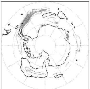
The sum (not shown) of the responses to the annular and the non-annular wind stress forcings (Fig. 11) is close to the response to the total wind stress forcing (Fig. 12) with only some minor differences, mainly located in the Indian and Pa-cific Sectors. Integrated over the whole Southern Ocean, the net effect of the mechanical (wind-stress driven) part of the SAM is a decrease in ice area that reaches a September value of about 530 000 km2(Table 2).
As the winter sea ice thickness is in the Weddell Sea every-where lower in the M+ run than in the CTRL run (due to the large response to the annular part of the forcing), the sum-mer sea ice area decreases sharply there because the thinner sea ice melts more quickly. The total differences in sea ice area between the M+ and the CTRL runs in summer (around 577 000 km2at the beginning of March) can be accounted for the most important part to these changes in the Weddell Sea (around 499 000 km2at the beginning of March). In the Ross Sea, the differences in summer sea ice area are small (around 7000 km2). In the other sectors (Amundsen-Bellingshausen, Indian and Pacific), the summer ice area anomaly is small in the M+ run, as almost all the ice is melted in both runs.
6 Conclusions
In order to extract the role of the wind stress and the air tem-perature forcing in the subdecadal response associated with the SAM, we have made a series of runs with a coupled sea ice-ocean model. In those experiments, an idealized anomaly based on the regression between the NCEP-NCAR reanaly-sis data and the SAM index has been added to the standard forcing, some of the runs with only the mechanical part of the anomaly of the forcing, others with only the thermal part of the idealized anomaly. We have seen that the thermal part (air temperature) resulted in more sea ice when the SAM in-dex is positive, because of the lower air temperature, mainly in autumn and winter except in the Weddell Sea and around the Peninsula where the warmer air temperature there is re-sponsible for a decrease in the ice concentration.
The response to the mechanical forcing (wind stress) can be decomposed into several different terms. The first one is related to changes in the ice velocity, which is largely due to the non-annular part of the mechanical forcing. This is responsible for the increase in ice area in the Ross Sea as it pushes ice away of the continent. The annular part in-duces higher upward oceanic velocities close to the Antarc-tic continent due to an increased Ekman pumping when the SAM is high. As a result, warmer water rises and the ice
Fig. 11. (a) Half of the differences in sea ice concentration at the end of July between Ann+ and Ann− for the first seven years of the
idealized simulations. (b) Half of the difference in sea ice concentration at the end of July between NA+ and NA− for the first seven years of the idealized simulations. Contour interval is 0.05. Solid lines are positive values, while dotted lines show negative values. Shading in dark gray means a value of more than 0.1, whereas shading in light gray shows a value of less than 0.1.
melts. The latter effect can be seen in the Indian, the Pa-cific, the Ross and the Amundsen-Bellingshausen Sectors. Another effect of this pumping is the rise in surface salinity in the Weddell Sea, which destabilises the water column. This results in an increased mixing layer depth and a lesser ice area. In addition, the mechanical forcing has an effect on the currents (northward surface currents and southward deeper in the ocean, pumping close to the continent, downwelling around 40◦S) and on the mixed layer depth (increased mixed layer depth due to increased wind stirring and locally to the increased upwelling) and the salinity.
When analysing the ocean currents, the results of the total forcing are, in general, very close to those from the runs with only wind-stress forcing. This is logical, as it is the wind stress and not the air temperature that forces the Ekman Drift. For the ice cover, the response to the SAM forcing can be explained as the sum of the responses to the distinct mechan-ical and thermal forcing. The combination of the two gives a dipole in winter, with less ice in the Weddell Sector and more ice in the Ross Sector (Fig. 4). The response in the Eastern Bellingshausen Sector follows the Weddell Sector, whereas the Western Amundsen Sector has a behaviour similar to the Ross Sector. In the other sectors, the decreases in sea ice concentration due to the enhanced pumping in the winter sea ice concentration are compensated by the increases due to the lower air temperatures. These changes are all in good agreement with the observations and with our previous ex-periments (Lefebvre et al., 2004) (Fig. 4). When integrated
Fig. 12. Half of the differences in sea ice concentration at the end
of July between M+ and M− for the first seven years of the ideal-ized simulations. Contour interval is 0.05. Solid lines are positive values, while dotted lines show negative values. Shading in dark gray means a value of more than 0.1, whereas shading in light gray shows a value of less than 0.1.
over the different sectors (Table 2), we see that the decrease in ice extent in the Weddell Sea and the increase in the Ross Sea is noticed in nearly all the runs. For those two areas, the thermal and mechanical effects tend thus to reinforce each other. On the other hand, mechanical and thermal forcing tend to have opposite responses in the other sectors, result-ing in weaker total changes. The responses to the thermal and mechanical forcing have more or less the same ampli-tude. This shows that, despite the low correlation between the SAM index and the air temperature, the thermal forcing could by all means not be neglected. This is due on the one hand to the large variability of the air temperature in the po-lar areas (low correlations are thus not associated with small temperature changes) and on the other hand to the strong im-pact of temperature changes on the ice cover.
Table 2 also illustrates that, integrated over the whole Southern Ocean, the thermal forcing induces an increase in the ice extent, while the mechanical forcing is responsible for a decrease of the ice extent. The latter is mainly due to the annular part of the forcing since the non-annular part is asso-ciated with an increase of the ice extent. Overall, the SAM is associated with an decrease of the ice extent in winter in our simulations. Nevertheless, the complexity of the geo-graphical distribution of the response and of the mechanisms involved with compensating effect of thermal and mechani-cal forcing imply that any long term influence of the SAM on the ice extent integrated over the Southern Hemisphere is very difficult to estimate from the available information. As a consequence, this integrated response could not be consid-ered as a robust model result at this stage.
Furthermore, we must keep in mind that our distinction between the thermal and the mechanical forcing is a bit arti-ficial. First, in the real world, changes in wind direction (and thus in wind stress) are generally associated with changes in air temperature. In this case, both wind stress and tempera-ture changes could be related to a common cause. Secondly, our experimental design does not allow to take into account any feedback between the atmosphere and the ice-ocean sys-tem. For instance, a change in the wind stress could induce a modification of the location of the ice edge and thus a change in air temperature that could amplify the initial response. By using our experimental design, those changes in wind stress and air temperature would appear unrelated while in this ample they are strongly linked. As a consequence, our ex-periments show clearly that both changes in mechanical and thermal forcing are important to understand the response of the ice-ocean system but we are not able in the present frame-work to determine the links between those two forcing or to analyse the way the atmospheric anomalies are produced.
Acknowledgements. This study is supported by the Federal Science
Policy Office (Belgium) (contracts EV/10/7D and EV/10/9A) and the Action Concert´ee Incitative Changement Climatique (Project Changement Climatique et Cryosph`ere) from the French Ministry of Research. H. Goosse is Research Associate with the Belgian National Fund for Scientific Research. The NCEP-NCAR
reanalysis data were provided through the NOAA-CIRES Climate Diagnostics Center, Boulder.
Edited by: D. Stevens
References
Berliand, M. E. and Strokina, T. G.: Global distribution of the to-tal amount of clouds (in Russian), 71 pp., Hydrometeorological, Leningrad, Russia, 1980.
Cai, W. and Watterson, I. G.: Modes of Interannual Variability of the Southern Hemisphere Circulation Simulated by the CSIRO Climate Model, J. Clim., 15, 1159–1174, 2002.
Connolley, W. M.: Variability in annual mean circulation in south-ern high latitudes, Clim. Dyn., 13, 745–756, 1997.
Fichefet, T. and Morales Maqueda, M. A.: Sensitivity of a global sea ice model to the treatment of ice thermodynamics and dy-namics, J. Geophys. Res., 102(C6), 12 609–12 646, 1997. Fyfe, J. C. and Saenko, O. A.: Human-Induced Change in the
Antarctic Circumpolar Current, J. Clim., 18, 3068–3073, 2005. Genthon, C., Krinner, G., and Sacchettini, M.: Interannual
Antarc-tic tropospheric circulation and precipitation variability, Clim. Dyn., 21, 289–307, doi:10.1007/s00382-003-0329-1, 2003. Gong, D. and Wang, S.: Definition of Antarctic oscillation index,
Geophys. Res. Lett., 26(4), 459–462, 1999.
Goosse, H.: Modelling the large-scale behaviour of the coupled ocean-sea-ice system, PhD thesis, 231 pp., Fac. des Sci. Appl., Univ. Cath. de Louvain, Louvain-la-Neuve, Belgium, 1997. Goosse, H. and Fichefet, T.: Importance of ice-ocean interactions
for the global ocean circulation: A model study, J. Geophys. Res., 104, 23 337–23 355, 1999.
Hall, A. and Visbeck, M.: Synchronous Variability in the Southern Hemisphere Atmosphere, Sea Ice, and Ocean Resulting from the Annular Mode, J. Clim., 15, 3043–3057, 2002.
Hibler III, W. D.: A dynamic thermodynamic sea ice model, J. Phys. Oceano., 9(4), 815–846, 1979.
Jackett, D. R. and McDougall, T. J.: Stabilization of hydographic data, J. Atmos. Ocean. Tech., 12, 381–389, 1995.
Kalnay, E., Kanamitsu, M., Kistler, R., Collins, W., Deaven, D., Gandin, L., Iredell, M., Saha, S., White, G., Woollen, J., Zhu, Y., Chelliah, M., Ebisuzaki, W., Higgins, W., Janowiak, J., Mo, K. C., Ropelewski, C., Wang, J., Leetmaa, A., Reynolds, R., Jenne, R., and Joseph, D.: The NCEP/NCAR 40-year reanalysis project, Bull. Am. Meteorol. Soc., 77, 437–470, 1996.
Kwok, R. and Comiso, J. C.: Spatial patterns of variability in Antarctic surface temperature: Connections to the Southern An-nular Mode and the Southern Oscillation, Geophys. Res. Lett., 29(14), 1705, doi:10.1029/2002GL015415, 2002.
Lefebvre, W., Goosse, H., Timmermann, R., and Fichefet, T.: Influ-ence of the Southern Annular Mode on the sea ice-ocean system, J. Geophys. Res., 109, C09005, doi:10.1029/2004JC002403, 2004.
Limpasuvan, V. and Hartmann, D. L.: Wave-maintained annular modes of climate variability, J. Clim., 13, 4414–4429, 2000. Liu, J., Curry, J. A., and Martinson, D. G.: Interpretation of recent
Antarctic sea ice variability, Geophys. Res. Lett., 31, L02205, doi:10.1029/2003GL018732, 2004.
Madec, G., Delecluse, P., Imbard, M., and L´evy, C.: OPA 8.1 Ocean General Circulation Model reference manual, Notes du Pˆole de
mod´elisation, Institut Pierre-Simon Laplace (IPSL), France, X, 91 pp., 1999.
Marshall, G. J.: Trends in the Southern Annular Mode from Obser-vations and Reanalyses, J. Clim., 16, 4134–4143, 2003. Mo, K. C.: Relationships between Low-Frequency Variance in the
Southern Hemisphere and Sea Surface Temperature Anomalies, J. Clim., 13, 3599–3610, 2000.
Oke, P. R. and England, M. H.: Oceanic Response to Changes in the Latitude of the Southern Hemisphere Subpolar Westerly Winds, J. Clim., 17, 1040–1054, 2004.
Rayner, N. A., Parker, D. E., Horton, E. B., Folland, C. K., Alexan-der, L. V., Rowell, D. P., Kent, E. C., and Kaplan, A.: Global analyses of sea surface temperature, sea ice, and night marine air temperature since the late nineteenth century, J. Geophys. Res., 108(D14), 4407, doi:10.1029/2002JD002670, 2003.
Simmonds, I.: Modes of atmospheric variability over the Southern Ocean, J. Geophys. Res., 108(C4), 8078, doi:10.1029/2000JC000542, 2003.
Thompson, D. W. J. and Solomon, S.: Interpretation of Recent Southern Hemisphere Climate Change, Science, 296, 895–899, 2002.
Thompson, D. W. J. and Wallace, J. M.: Annular modes in the Extratropical Circulation. Part I: Month-to-Month Variability, J. Clim., 13, 1000–1016, 2000.
Timmermann, R., Goosse, H., Madec, G., Fichefet, T., Ethe, C., and Duli`ere, V.: On the representation of high latitude processes in the ORCALIM global coupled sea ice-ocean model, Ocean Mod-elling, 8(1-2), 175–201, doi:10.1016/j.ocemod.2003.12.009, 2005.
Trenberth, K. E., Olson, J. G., and Large, W. G.: A global ocean wind stress climatology based on the ECMWF analyses, Na-tional Center for Atmospheric Research, NCAR/TN-338+STR, 93 pp., NCAR, Boulder, USA, 1989.
Watterson, I. G.: Southern midlatitude zonal wind vacillation and its interaction with the ocean in GCM simulations, J. Clim., 13, 562–5783, 2000.
Watterson, I. G.: Zonal wind vacillation and its interaction with the ocean: Implication for interannual variability and predictability, J. Geophys. Res., 106, 23 965–23 975, 2001.
Xie, P. and Arkin, P. A.: Analyses of global monthly precipita-tion using gauge observaprecipita-tions, satellite estimates and numerical model predictions, J. Clim., 9, 840–858, 1996.