Contracting force fields in robot navigation and extension to other problems

Contracting Force Fields in Robot Navigation and

Extension to Other Problems

by

Alexandre F. HAAG

Ingenieur de

l'Ecole

Submitted to the Department of Mechanical Engineering

in partial fulfillment of the requirements for the degree of

Master of Science in Mechanical Engineering

at the

MASSACHUSETTS INSTITUTE OF TECHNOLOGY

June 2000

@

Massachusetts Institute of Technology 2000. All rights reserved.

A uthor ...

Department of Mechanical Engineering

May 5, 2000

-/ /

Certified by...

Jean-Jacques E. Slotine

Professor of Mechanical Engineering and Information Sciences

Professor of Brain and Cognitive Sciences

Thesis Supervisor

Accepted by ...

Ain A. Sonin

Chairman, Department Committee on Graduate Students

MASSACHUSETTS INSTITUTE OF TECHNOLOGY

SEP

2000

Contracting Force Fields in Robot Navigation and Extension

to Other Problems

by

Alexandre F. HAAG

Submitted to the Department of Mechanical Engineering on May 5, 2000, in partial fulfillment of the

requirements for the degree of

Master of Science in Mechanical Engineering

Abstract

This thesis derives results in path planning and obstacles avoidance using force fields. Based on Contraction Theory, we prove convergence of a simple attractive force field. Repulsive fields are , in general, not contracting in the Euclidean metric, but we can define a contracting region when it is combined with another contracting field. We then provide interesting results about superposition and combination of many force fields. This theory also enables us to simply extend these convergence properties to non-autonomous systems such as moving obstacles.

Next, we apply successfully breadth first search, dynamic programming and fast marching method to create global force (or potential) fields. We compare these three techniques, explain that there are in fact almost equivalent and present solutions to improve their computational efficiency. This thesis also addresses the extension to much more general problems than robotics, especially in optimization, and exposes an original solution to the Traveling Salesman Problem that runs in o(N22').

Finally we introduce a new mathematical distance as a theoretical tool to better understand the structure of the workspace. We present general results that will help find more theoretical results about superposition of force fields . An efficient algorithm that uses the sum of previously computed potential fields to build a new one is given. As an application, we describe an implementation of a concurrent mapping and localization problem on a simulated Khepera robot. We give some insights on the problem and in particular we explain how to do very simply a gradient descent with a real robot on our virtual potential field.

Thesis Supervisor: Jean-Jacques E. Slotine

Title: Professor of Mechanical Engineering and Information Sciences Professor of Brain and Cognitive Sciences

Acknowledgments

I would like to express my gratitude to my advisor, Professor Jean-Jacques Slotine. He was a good source of support and ideas and he let me the freedom necessary to be inspired by the muses of creativity.

Special thanks go to my very close lab-mate Caroline, with whom I had a lot of interesting discussions on our research problems. My other lab-mates Lutz, Martin, Winnie and Jesse answered many questions I had and I thank them very deeply.

I furthermore appreciate the friendships I have found here: Gwenaelle, Jeff, Jeremy, Maxime, Gilles, Frank, Stephane and many others. They all provided numerous pieces of advice and comments and made this time thoroughly enjoyable.

Finally, I am very grateful to my whole family who supported and encouraged my work.

Contents

1 Introduction

2 Local Obstacle Avoidance

2.1 Attractive Force Field . . . .

2.2 Repulsive Force Field . . . .

2.2.1 One, Basic Repulsive Point . . . .

2.2.2 More Complex Repulsive Force Fields

2.2.3 Many Repulsive Points

2.2.4 Repulsive Region . . .

2.2.5 Moving Obstacles . . . 2.2.6 Combination . . . . .

2.3 Conclusion . . . .

3 Global Path Planning

3.1 Introduction . . . .

3.2 Three Different approaches . .

3.2.1 Graph Search . . . . . 3.2.2 Dynamic Programming 3.2.3 Fast Marching Method 3.3 Comparison . . . . 3.4 Improvement

3.5 Example: the Traveling Salesm

3.6 Link to PDE theory . . . .

an Problem

4 A New Metric on the Workspace

4.1 Motivation . . . . 4.2 Definition . . . . 4.3 Properties . . . . 4.4 Applications . . . .

4.4.1 Superposition of potential fields

4.4.2 Convex functions . . . . 4.4.3 An efficient algorithm . . . . 6 9 9 11 12 14 17 18 19 19 22 23 23 24 24 25 26 27 28 30 33 35 35 35 36 37 37 40 40

5 Application : Concurrent Mapping and Localization 42

5.1 Introduction . . . . 42

5.2 Application of previous theories . . . . 43

5.2.1 Exploring Phase . . . . 43

5.2.2 Repositioning Phase . . . . 44

5.3 R esults . . . . 45

Chapter 1

Introduction

By force field we understand a function that to each state assigns a precise control. For a robot moving in the plane, this function can be viewed as a vectorial force, which makes the robot move. Even though we will often use the representation of the robot here, it is important to keep in mind that almost all results may be applied to more general cases like optimization or other graph search problems.

If this force field F has no vorticity, which is usually the case, there exists a scalar

function 0 such that its gradient is the desired force field F. # is called an Artificial

Potential Field. Its use is one of the most efficient approaches for online obstacle avoidance to date and has been introduced by [9] and studied by many others. We will not make a big distinction between the scalar and the vectorial approaches in the following and, for example, an equilibrium point will be described either as a minimum of the potential field or as a zero of the force field.

The idea of seeing a control algorithm as a force field in the work -Cartesian- or joint space of the robot is several years old. But some biological experiments have brought new interest in this theory.

Many researchers have suggested a hierarchical control scheme for movement con-trol, based on arguments of bandwidth (there are many sensors and muscles which need a large amount of information to function correctly), delays (nerves are slow, and communicating all that information would result in long delays, with subsequent control problems), and anatomy (the loop from muscles to spinal cord to sensors sug-gests heavily some low level control modulated by descending signals from the brain).

Experiments by Bizzi [3] and others (Giszter [7], Mussa-Ivaldi [15] and Loeb [12])

have attempted to elucidate this hierarchy. They electrically stimulated the spinal cords of frogs and rats and measured the forces obtained at the leg, mapping out a force field in leg-motion space.

Surprisingly, they found that the fields were generally convergent (with a single equilibrium point) and uniform across frogs. The idea is that if the leg is free to move,

it will move to the center of the force field, see Giszter [7]. Different fields therefore

correspond to different postures.

They have found that the fields can be combined either by superposition -stimulating in two places in the spinal cord resulted in a field which is the linear vector superpo-sition of the fields obtained when each point was simulated, or by "winner-takes-all"

- stimulating in two places and finding the resulting field coming from one of the two

places (Mussa-Ivaldi

[15]).

is deafferated (Loeb [12]), which strongly suggests that the fields are caused by the interaction of the constant (there is no sensory feedback) spring-like properties of the muscles and the leg kinematics.

These findings lead researchers to suggest that these fields are primitives that are combined to obtain leg motion. Mussa-Ivaldi and Giszter [14] have shown that fairly arbitrary force patterns and so complex motions can be generated using a few of these force field primitives. This theory sounds very attractive to robotics engineers, whose realizations have performances far from those of the animal world.

From the Artificial Intelligence point-of-view now, there are three main reasons to use force fields or motion primitives: it is supposed to be quite simple to implement, computationally efficient and as powerful as animal motions. Furthermore, since it is working in real world on animal, we can expect that it will work on robots! The problem remains to find out more precisely how to use force fields and how to prove their convergence and stability.

From a control point-of-view, force field theory can be seen as a convenient and efficient way to plot and visualize the control policy at each state point.

Contraction theory has been introduced by Lohmiller and Slotine [13] recently. Intuitively, contraction analysis is based on a slightly different view of what stability is, inspired by fluid mechanics. Regardless of the exact technical form in which it is defined, stability is generally viewed relative to some nominal motion or equilibrium point. Contraction analysis is motivated by the elementary remark that talking about stability does not require one to know what the nominal motion is: intuitively, a system is stable in some region if initial conditions or temporary disturbances are somehow forgotten, i.e., if the final behavior of the system is independent of the initial conditions. All trajectories then converge to the nominal motion. In turn, this shows

that stability can be analyzed differentially - do nearby trajectories converge to one

another?- rather than through finding some implicit motion integral as in Lyapunov theory, or through some global state transformation as in feedback linearization. Not surprisingly such differential analysis turns out to be significantly simpler than its integral counterpart.

To solve the obstacle avoidance problem, we start by presenting basic calculations on force fields (chapter 2). Our aim in this chapter is to prove what kind of attractive and repulsive force fields are contracting and how we can use them for more complex problems (multiple obstacles, non-punctual obstacles and time varying environment). All these results apply more at the low or local level, in cases where an entire path is already planned at the global level. This is actually what chapter 3 is about: global path planning. We first present existing techniques to find efficiently a trajectory and the shortest path from one point to another in a maze or in more general problems. These techniques are Breadth First Search (BFS), Dynamic Programming (DP) and Fast Marching Methods (FMM). We show that they are almost equivalent and that they still can be improved. In particular we apply this improvement at the end of this chapter to an original modeling and efficient solving of the Traveling Salesman Problem. This is an algorithm that finds an exact solution of problem up to 26 cities

in less than a minute. Chapter 4 introduces a new metric on the workspace and tries to build new mathematical tools useful for convergence and stability analysis. It derives general theoretical results and also presents a new fast algorithm to find a path from one point to another in a maze, by reusing the computation done before to plan other trajectories. We end this thesis with an application of some of the previous results: a concurrent mapping and localization problem is implemented on a simulated Khepera robot. The robot is exploring randomly its unknown environment, building an internal map at the same time and then using it to navigate to a desired position.

Chapter 2

Local Obstacle Avoidance

Obstacle avoidance is the problem of designing a controller that safely navigates the robot around forbidden points to avoid collisions. By local, we mean that the results presented in this chapter apply more to the cases where the main goal of the robot is to go to one "close" point (the attractive point), avoiding a few obstacles (the repulsive points). For example a really complicated maze will be better solved using other techniques like the ones presented in chapter 3.

Here, we will show that the superposition of simple radial force fields works very well and is a very simple way to design control functions. Based on a new method to analyze stability (contraction theory [13]), we perform a separate study of different fields. Next, we propose different applications of the superposition of these fields: multiple obstacles and repulsive regions. Furthermore, the contraction theory and

the use of the variable s = x + T± enable us to derive very easily similar results for

non-autonomous systems or moving obstacles.

The work presented here is done for a mass-point robot in a Cartesian space. But as long as its equation of the dynamic is similar to (2.2), another system can be solved with the same approach. For example, manipulator robots could use those techniques for their end effectors and one of the obstacles would be the arm of the robot itself. The calculations are usually done in two dimensions but we show how to extend the results for n-dimensional problems.

2.1

Attractive Force Field

An attractive point is used to set the goal the robot has to reach.

We present first the simplest case: there is only one attractive point and no obstacles in the environment (at least locally). Moreover we consider the robot as a mass point.

Let us first introduce a new variable, s, which acts as a prediction of the position of the robot T seconds further, by including the velocity:

s= x + T - - (2.1)

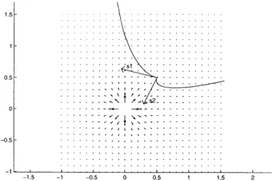
0.5 - -- - - - -- - - - 0-S /I f t I -0.5 110 /1 / ,- / //I / f t I I IS, I .- S--AA.-',/ I/ I f f t t t I I\ \\~ .1 ///// ////// / / f t t t t I \\ -1 -0.5 0 0.5 1 1.5

Figure 2-1: An attractive force field centered in (0.5, 0.5) with two initial vectors s and corresponding trajectories followed by the robot, according to equations (2.1) ,

(2.2) and (2.3). Here T = 1.

T can also be seen as a factor that changes the relative importance of damping and

stiffness: the higher T, the higher the damping in the motion. There are many benefits in using s. First we manipulate only a single variable instead of both the position and the velocity and moreover this will enable us to transform a second order system into a first order system. Secondly, the damping is embedded deeper into the control equations. Third, it is easier to use in contraction analysis. The introduction of the s variable is also related to the Sliding Control Theory [20].

We then have the fundamental equation of dynamic:

F(x) = m - i (2.2)

where F(x) is the force field created to control the robot and m the mass of the robot. Finally, we can chose the control F(x) applied to the system by another vectorial function f (s)

F(x) = m - (f (s) -

±)

= i + T. = f(s)

which is the usual form for a control equation. It is also a first order differential equation. This means that s is controlled by a velocity field instead of a force field for x. It is thus much easier to visualize the behavior of the variable s: it just follows the stream lines. For example, on figures (2-1), (2-2) and (2-3), the trajectories of s are just straight lines from the starting point towards the attracting point or away from the repulsive point.

From there, we can apply the contraction theory [13], which states that the pre-vious system is contracting if :

1 f + fT

2 Os Os

--For an attractive point, we chose : (the size of the square matrix K is the number of dimensions of the space)

ki 0

f

If ki, k2, .-. > ₁ > 0 , then the system is contracting and every trajectory s(t) tends

to so. This means that two different trajectories with initial conditions s1(0) = sol

and s2(0) = sO2 will converge to the same trajectory so(t).

Now we can go back from the s state space to the (x, 1) state space. By looking at the definition of s, we see that x is defined by a first order differential equation

x + T± = s(t), which implies exponential convergence to a particular solution of

the differential equation. Thus two trajectories in (x, sb) with two different initial conditions, will converge exponentially to two particular solutions that converge to

the same solution (i.e. the solution of x+ Tb = so (t) ), which implies that the system

has also a contracting behavior in x.

Another important question is how to choose the value of T. Basically, we do not want s to be "too far" from x, so that the behavior of the real robot (x) is not too far from the controlled variable, s; but at the same time we want T not too small to

use the prediction effect of s .What we mean by "too far" depends of course on the

scale of the problem: if the distances in the environment are small or if everything is

moving fast, T has to be small. For example, in our simulations we used T = _{j, in a}

2x2 environment, with obstacles moving at a speed of 0.5.

For a basic attractive force field as in figure (2-1), so is just defined by so = xo,

the center of the field. But the above demonstration is also valid for non autonomous systems where the center of the force field is moving, that is where s depends on t.

Since the contraction is conserved by addition, the sum of different force fields, contracting within the same metrics, is still a contracting field. In particular, we can add two attractive force fields and get a new attractive force field centered elsewhere. We do not know whether the force fields discovered in the frog are mathematically contracting, but motion primitives are a typical application of the previous result.

2.2

Repulsive Force Field

Repulsive points represent the obstacles the robot has to avoid. As it will appear in this section, repulsive force fields are much more complex than attractive ones: contraction is not straightforward and they can create local minima in the field.

2.2.1 One, Basic Repulsive Point

We assume the repulsive point is at 0. For a repulsive force field centered at another

point, we may just consider s - so instead of s .

At the difference of the attractive case, the repulsive force field should have very low influence far from the center. The first function that comes to mind is something

SF

linear and as simple as f(s) =0 otherwise k. There is a problem with

this though. It is due to the fact that the control function depend on s and not directly on the position. This means that we apply to the robot the force corresponding not to where it is but to where the vector s points. Thus, for example, if the robot is on one side of an obstacle and s already points across the obstacle to the other side, the field will attract the robot towards the repulsive obstacle! To avoid that, we assume that this is not the case at time 0 and need to set the force to infinity at the center of the obstacle to ensure that the robot will always be sufficiently slowed down when

approaching an obstacle' . The 1/r function is then a logical continuous function to

use.

We still use the same definition of s as in (2.1) and the same equation for the control (2.3) as in previous section. Then if we choose the basic radial repulsive field

f(s) = ' , the derivative of f is (in 2D, where s. and s, are the two components of s ):

2 s 2sYs which is not definite negative. Therefore we can-not conclude to the contraction of such a field. It is actually obvious on a plot-out that a basic repulsive force field is not contracting and that any trajectory is going away from any other.

Even though, if we make a metric change and look at the same trajectories in polar coordinates (figure 2-3), we see that the trajectories are "not too far" from being contracting. Actually the trajectories of the s variable are horizontal straight lines, which stay at the same distance in 0 from each other and tends to the same r. They do not contract to a single trajectory, but they also do not diverge from each other. Therefore, we had the idea that the presented repulsive force field is "almost" contracting and that when added to a strongly enough contracting field, the sum remains contracting.

To prove this mathematically, we look at the eigenvalues of the symmetric part of

f

the region too close to the repulsive point, Arep is upper bounded on the domain by,

let's say, Arepmax. A contracting force field is characterized by a symmetric part of

it's Jacobian, Jcont, , which is definite negative. Then Jcontr is diagonalizable and

its biggest eigenvalue Acontr max is negative. To verify if the sum of the two fields

is contracting, we check whether the sum of the symmetric parts of the Jacobians, expressed in the same metric, is definite negative. We have :

'For a real robot, the force can not be infinite and it is important to change appropriately the controller in case s would point to the other side of the repulsive point.

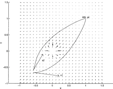
1.5 - - - -0.5 0 - -- - - -- - -. - - - - -.-.--0.5 - - - - - -. -. -. . . . .. . . . -1L -1.5 -1 -- 0.5 0 0.5 1 1.5 2

Figure 2-2: basic radial repulsive force field with two initial vectors si and s2 and the corresponding trajectories followed by the robot.

1.8 - - - - - -- ---1.6 -1.2 --- - - - - - - - - - - - - - - - - - - - -0.8 -0.6 -0.4 - s2 0.2 -0.5 1 1.5 2 2.5 r

Figure 2-3: Same as figure (2-2) but in polar coordinates. Note that the trajectories for s are horizontal straight lines.

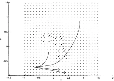
1.5 - - - - -0.5- - 0-- - - . s2. -0.5- - -Si -1 -0.5 0 0.5 1 1.5

Figure 2-4: The two trajectories "contract" to the same point on this force field consisting of a basic attractive field and a basic repulsive field.

Vx Z 0, XT JcontrX < Acontr maxIX12 < 0

Vx 5 0, xT JrepX < ArepmaxIX1|2 _{< Arep1JX1}2

thus, Vx = 0, XT(Jrep + Jcontr)X < (Arepmax + Acontr max)IIXH12

Then a sufficient condition for the system to be contracting is

(Arepmax + Acontrmax) < 0 . This can be achieved either by strengthening the

contracting force field (more negative Acontrmax ) or weakening the repulsive force

field (smaller Arepmax _{) or increasing the size of the excluded domain around the}

repulsive point. In the last case however, if the contracting field is an attractive one, it is better not to exclude this attractive point from the contracting domain. It is also interesting to note that the region excluded could correspond to the real size of the non-punctual obstacle. Finally, since the non-contracting region is repulsive and bounded, any trajectory starting in this region is going to its boundary and then to the contracting domain; and this also guarantees that any trajectory starting in the contracting domain will end up in it. Figure 2-5 shows the importance of this second condition; the trajectory can go out of the contracting domain, in which case the distance between two trajectories is not necessarily decreasing, but it will return to it after a finite time. Thus every trajectory ends up at the desired attractive point.

This result is confirmed by simulations and can be viewed on figure 2-4.

2.2.2

More Complex Repulsive Force Fields

First Note that the equilibrium point does not correspond exactly to the center of the attractive force field because the repulsive field has still a small influence at this point.

Thus once a target point and an obstacle are defined, the equation fattr(X) = frep(X)

must be solved to find the position x at which the attractive point has to be set. A simple way to avoid that is to continuously cancel the repulsive force field outside

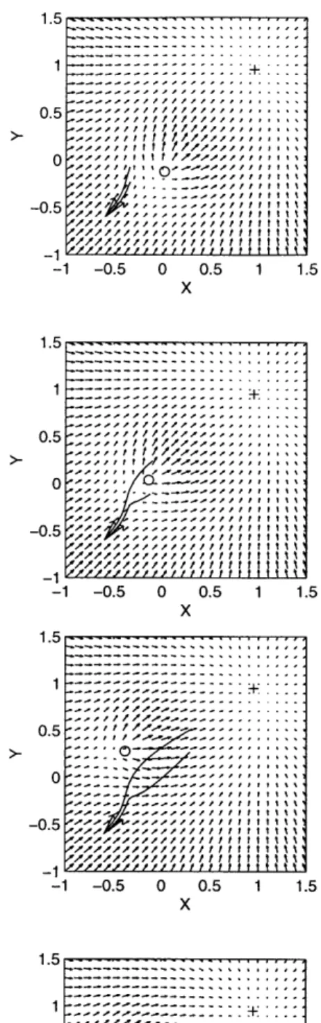
- - -- - - - - - . . . . /// / I I f I I I I N \ / / / / I 0 . 1 1 .5\ -1 -0.5 0 0.5 1 1.5 -1 -. 5 0 0.5 1. 1.5- 0.- -0.5-1.5 0.5 0 -0.5 -1 -0.5 0 0.5 1 1.5 Sx 0.9 -0.8 0.7-0.6 -0.5 - 0.4- 0.3-0.2 - 0.1-0 1 0 20 30 40 50 60 70 so Time - - - -- - - - - -.4I) -I/I I t I r t I tt '/ / / I I f f I -'///// / / / / / / 1t

Figure 2-5: The top plot shows the trajectory in (x,y) coordinates; the middle plot

is in the s = (sr, sy) space and the bottom one is the distance between the two

trajectories over time. One can see that when one of the trajectories is leaving the contracting domain (outside the circle), the distance can increase.

1.5

-- - - - -- - - - -

-a given b-all of influence. We c-an, for inst-ance use the function f(s) = max( s

-R,' 0). The eigenvalues of the symmetric part of the Jacobian of

f

ball of radius RO, the same as in the previous subsection (Arep = t 1) and are null

outside. We could construct a function that would have the same properties and that is moreover smooth but this does not seem to be necessary.

Another thing we want to take into account is the size of the obstacle. Since in real

world, obstacles are not points, we propose the following function: f(s) = _,I

s > ro, which is explained in more details in the section "Repulsive Region".

Also, It is easy to verify that this result is valid for an N-dimensional space. In

fact, the eigenvalues of the Jacobian are still Arep = , the positive one being a

(N-1)-order eigenvalue.

Finally, if we change the reference frame and use the cylindrical coordinates (r, 0), we have the new expressions of the different equations:

s 8 - M- cos 0 sin 0 sX

r - x - _-sin0

cos 0 _sy

expressed on r, 0: so =

,

-Tr ro + O

the fundamental equation of dynamic in cylindrical coordinates becomes:

Fro = m

(

now it appears that if for the control, we use:

Fro =-f(s) - m T

)

T -r0

then combining these equations leads to the equation of the system is: Ar9 = frO(SrO),

which without subscript is the classical form for a control equation:

=

±

f(s)

Now, let's assume

fro =

(-S

where 6 > 0. we choose E very small so that it is significant from a mathematical

point of view but negligible in practice.

Then fro is contracting and the system is contracting for 0 f 7r and the use of

1

means the field is repulsive. By adding another term A =

(

)

1.5r -1 - - - - - -- --0.5 -1 - 1 .5 1. 0 . . . . . -.5 -1.5 -1 -0.5 0 0.5 1 1.5 2 X

Figure 2-6: Existence of a local minimum in front of a group of three obstacles: The trajectory whose initial s is in the non-contracting domain ends up in a local minimum.

this metric is not really practical when there are other force fields centered elsewhere. Indeed the trajectories in a basic attractive force field (straight lines in Cartesian

space) are acos functions in the (r, 0) metric centered at the repulsive point: there

are not contracting in the whole space.

2.2.3

Many Repulsive Points

To represent other obstacles in the environment, we add other repulsive force fields. Almost as before, they will be described by the function f = (I ) , where si is

the center of the repulsive force field number i. The eigenvalues of the corresponding

Jacobian are Arep_i = ± 1 The system is then contracting in a given domain

if we have at each point inside this domain: (Acontr + E Arepi) < 0 . This equation

defines the contracting domain and as in the previous section, it can be modified by

strengthening the contracting force field (more negative Acontrmax ) or weakening the

repulsive force field (smaller Arep ).

The main problem with multiple force fields is the possible existence of local minima different from the global minimum (figure 2-6). But in our case, the previous proof ensure us that any local minimum is outside the contracting domain, because there can be only one equilibrium point in a contracting domain. Therefore if the robot starts in the contracting domain (which is easy to check) and it remains in it then it will go to the attractive point. In this case, the difficulty is to predict whether the robot will remain in this contracting domain or not. However, we know that if the robot starts in a ball centered at the equilibrium point and included in the contracting domain, it will always remain in this ball and contract to the equilibrium point.

To avoid local minima, there also exist the solution of using harmonic functions as potential field. Harmonic functions are functions whose second derivative verifies

1.Sr 15r . .. . . . . . . . 0 . I f i "p. sitio"of . 0.5 0 .0 . -0. . '2. . . - .5. . . . . . . . . 1. . . . . . . . 1 . . . . . . . -1 .5 0 05 1 15 -1 -0.0 0 05 1 1.5 0 0

Figure 2-7: Importance of initial "position" of s. On the left plot s points to (-0.01,

-0.01) and in the right plot s points to (0.01 0.01).

the Laplace equation V2o = 0. See [6][4][10], for instance, for more precise results

on harmonic functions. Their use comes from the fluid analogy and they have the fundamental properties that first the sum of two harmonic functions is still an har-monic function and secondly that they achieve their extremum only on the boundary

of objects. In two dimensions,

#(X)

harmonic function (k is positive for an attractive potential field and negative for a repulsive one). We can see that the repulsive force fields we used before are harmonic:

grad = 1/r . Unfortunately the attractive force field presented at the beginning of the chapter (equation (2.4)) is not harmonic, thus we cannot conclude anything about

their sum. If we use for the attractive force field f(s) = - the sum is a harmonic

potential, but this field is not contracting. This is easily proved by remarking that the trace of the Jacobian of any Harmonic field is null (by definition) and by the fact that changing the metric does not change the trace (if the metric change does not

depend on time). Thus at least one of the eigenvalues of the Jacobian is positive or

null.

In an n-dimensional space a typical harmonic potential is O(X) = k * )n/2

These kinds of fields are a bit different from the - fields proposed in the previous

subsection, but their greatest eigenvalues are still bounded by ( and thus we

can apply the same proof to get the contraction property.

2.2.4

Repulsive Region

One idea here is to use many repulsive points to model a repulsive region instead of just repulsive points. The problem is to define where the robot can go between two points and where it can't because it is supposed to be the same obstacle. In other

words we have to find out how many points are needed to represent one obstacle.

By the way, we also have to check that if two obstacles are close but not enough to

block the robot, this representation of force fields will allow the controller to drive the robot between these two obstacles. Figure 2-7 shows the kind of problems we may

encounter when there are two repulsive points. It also reminds us that when using the s variable, it has to point outside a forbidden domain at the beginning.

Another solution is to use functions that are infinite on the border of the obstacle, so that the robot can never get inside the region defined by the obstacle. For a circular obstacle, a good function will be f(s) = -Sq where so is the center

I I S-S i12 -R2

and R the radius of the obstacle. In the same way as in the previous section, we can show that this field is contracting when added with an attractive force field, except in a disk around the obstacle. The radius of this disk is the same as previously

plus R . This is easily shown by noting that the eigenvalues of the Jacobian are

A - 1 11 S-Sq 2±+R

2

Arep = S_,S-o 2-R2, (1S-soI 2-R2)2 , that the second one is always negative and that

the first one is bounded outside a disk of radius greater than R.

2.2.5

Moving Obstacles

This is one big advantage of contraction. Indeed the contraction theory tells us that if a non-autonomous system is contracting at every time then it is also contracting over time. This comes from the fact that we are only looking at the Jacobian, which contains no derivative over time. Thus all the previous results are valid if the attrac-tive point is moving (interception problem or movement defined by a global planner) and/or if the repulsive points are moving (the obstacles may represent people walking on the sidewalk and the robot has to avoid them). Since the velocity of the attractive or repulsive point is embedded in s, it does not change anything in the equations!

Moreover the center of a repulsive or attractive field is in so = xo

+

where the obstacle or the target is now, xo , but where it will be in T sec. Thus this

simple controller naturally looks ahead to detect a possible collision and avoid it. Figure 2-8 shows different shots of trajectories of robots avoiding a moving obsta-cle.

Since the non-contracting region is also moving with the obstacle, it may be more difficult to check that the robot does not stay in it. But for example, in the case where there is only one repulsive point and one attractive point, there is still no other stable equilibrium point than the attractive one.

2.2.6

Combination

Now that we have enough material on repulsive and contracting force fields, we can address the issue of choosing T exposed in section 2.1. The problem is that T defines for how far in time the prediction is made and is chosen more or less arbitrarily. Or for one given T, the robot may not see an obstacle that appears very close at the last moment or may "forget" an obstacle, if T is too high. On the other hand, if T is too low, the prediction is not enough ahead in time and the robot may detect obvious collisions only at the last moment. Thus it would be useful to be able to use different

variables si corresponding to different time T. Let us do it for i = 2. We have then

the two following contracting systems:

--- '.l-lt-I. i t//, / / 1t // fftI ,l ,, , / f f f I 1 0.5 0 -0.5 1 0.5 0 -0.5 -1 - I -1 -0.5 0 0.5 1 1.5 x 1.5 1 0.5 0 -0.5 _-1 -1 -0.5 0 0.5 1 1.5 x 1.5 0.5 0 -0.5 -1 -1 -0.5 0 0.5 1 1.5 x 1.5 1 0.5 0 -0.5 -1 -0.5 0 0.5 1 1.5 x 1.5 1 0.5 0 -0.5 -1 -1 -0.5 0 0.5 1 1.5 x 1.5 . 1---0.5- -- O~ -0 I f t I I AAA/A//// / 1111ff111 -1 -0.5 0 0.5 1 1.5 x -1 -0.5 0 0.5 1 1.5 x 1.5 1--- -1 - ,/ - -- - - - . 0.5 -- 0-.~..~~,,/1il I I~f -1 -0.5 ///... /A//1i 1ffff1 ..A, //p / 1/ It I IIf 1I /AA////////I 1111ff$111 1 //A/////////lf itilf t -1 -0.5 0 0.5 1 1.5 x

Figure 2-8: Read from left to right and top to bottom to see two different trajectories of a robot trying to avoid the obstacle represented by the small circle. The two trajectories are very close at the begining but one "prefers" to slow down at go

t it t I I f t111 I, I H'...-. - /111It 1111ff I ./ ///////,;,/il/ 1111 '/////) l//i liP111 f111 -o 4.... - /1 I t t I t -I I tt I t f f I -1 - - t1 -I11f f II ,///////,1Il I P/A/1/iiI. -- ----... -11/A... --- / A- --- -. --.. / it It t Ift it t t /A.IA///1 111 11ff f_{I/f/t 1 f t f} t t I I I I I oi/ I tI t t 1 -- ---. 0 - --.~~.li i IIII ~~/ ii tl f t l III It//tl1111 f AA//p'p1./~/// 11ff ff11 I A///A//A////I lIltl ff It . 1.5 1.5 i

where si x + TX' and where

f

S+ 2 . T₁ + T₂ .. fl(s1) + f2(s2)

2 = i + 2 = (2.7)

2 2 2

which, plugged into the equation of dynamic (2.2), gives the equation of control to apply to the robot:

F(x) =-= m 2 ( 81) + f2(S₂) (2.8)

T1 + T2 2

Thus, we can see the system (2.7) as :

(S = 1 + S2

S=fi(Si)

We want to guarantee the contraction of the system when both si and S2 are in the

contracting domain of fi and f2. To do that we express the system as the combination

of:

{+

S

which can be written:

/ _ 1

(

6 2 J T 1

+T2

Note that, in general, this is a block matrix equation if the dimension N of s is greater than one, which is usually the case. The l's are actually identity matrices for N > 1. But let us first consider the case where s is a scalar. The symmetric part of J has

[T19f + T2 fM - 2

2(T 1 + T2) Os, 9s2

t\

_{\T 09si +2}

82 +2 _{1si + 2aS2}

for eigenvalues. Since a real symmetric matrix is always diagonalizable, we are guar-anteed that the term under the square root is positive. However it is much harder

to prove that the two eigenvalues are negative. A 3D plot of the function A(Q, h)

other or when one of them is positive, in all other cases, which are also the most common, the greatest eigenvalue is negative and thus the system is contracting. In the other cases, we will need to find a new metric in which the system might be contracting (so far, we have not find simple metric that works).

For the general N-dimensional case, we have to consider J as a block matrix and the eigenvalues as matrices. These depends on the Jacobians f and their trans-poses. Then the same base change matrix expanded by block from 2x2 to 2Nx2N will

transform the symmetric part of J into

(

A, and A2 are definite negative so is T ₂ and the system is contracting.

2.3

Conclusion

Force field is a very efficient, useful and practical method for environment with few obstacles or when looking only at a region that has few obstacles (local problem). Moreover, with the contraction analysis of these force fields it is straight forward to derive similar convergence results for non-autonomous systems. Since the attractive point can move too, force fields could serve as a low-level controller that follows a defined trajectory. But to plan this defined trajectory or to control a robot in a bigger, more complicated environment, we need, to avoid local minima, to have a global approach and to use other techniques, which are presented in the next chapter.

Chapter 3

Global Path Planning

3.1

Introduction

This chapter starts with a presentation of three different efficient methods used in path planning, namely Breadth-First Search, Dynamic Programming and Fast March-ing Method. Then we compare them and show small advantages of each. But the main result of the first sections is that these three algorithms are actually almost identical and that their differences reside only in details of implementation and in their representations. This allow us to keep only one representation, which is almost that of Fast Marching Method: a potential field over the state space, which gradient can be viewed as a force field and that has only one minimum. The next section proposes an improvement of these algorithms, which is particularly interesting when the dimensionality of the problem is high. As an application of this remark, we solve the Traveling Salesman Problem using an original modeling, viewing the state space as an hypercube.

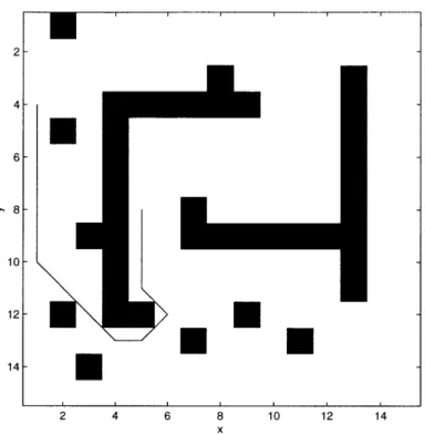
In order to have a concrete problem to talk about, we will present here the problem of a robot in a maze trying to find the shortest path from one point to another (figure 3-1). The maze is defined by a grid with obstacles (0 if free space or 1 if there is an obstacle at that point) or with costs to go to the next grid point (positive real numbers defining the cost at each point). When talking about mazes, we mean general ones, not those that have only one solution to go from the entry to the exit (those

problem have little interest ! ). There are two main differences with chapter 2: first

the problem is now a discrete one and second, the force defined by the field does not exactly correspond to the one that could appear in an equation of dynamic like (2.2) but more to a direction to the next state. But of course it is fundamental to keep in mind that the interest of this theory is that it can be extended to virtually every problem that can be transformed into a graph on which the best decisions have to be made at each successive state.

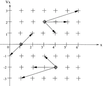
For example, if considering the previous problem as a dynamic problem (e.g. controlling the acceleration and not the displacement at each step), the velocity must be introduced in the state. Therefore a state is no longer defined as a position (x, y) but as a 4D state (x, y, vX, vy). It is a bit harder to represent and a slice of the state

E

U

I-U

U

I

U

Figure 3-1: The shortest path from (1,4) to (5,8).

space (figure 3-2) shows that the metric is all but Cartesian: two neighbor points in the sense of this problem (two states that can be successive) are not necessarily neighbors in the common sense. But we can still imagine a "robot" searching a shortest path in this 4D maze. We can also introduce the time as a 5th dimension, which enables to have a time dependent environment: moving obstacles are just as easy, if we know in advance how they will be moving. Another possible extension is the introduction of the probability. In this case the maze is not represented by zeros and ones whether there is an obstacle or there is not one, but by any number between zero and one representing the probability that there is an obstacle. These numbers will then be used as costs for the algorithms.

3.2

Three Different approaches

The aim of this section is to show that three different, well-known types of algorithms, with three different origins and representations have actually the same fundamental structure (i.e. the same order of computational time, same way of going through every point on the grid, only explanation and details on implementation are different).

3.2.1

Graph Search

The breadth-first search explores a graph G=(V,E) across the breadth of the frontier between discovered and undiscovered nodes. The later a node is examined the more distant it is from the starting node s.

10

12

Vx

22 3 4 5 6±

Figure 3-2: This is a cut of the 4D space (x, y, vo, vy) corresponding to the maze

problem with dynamic. It shows the neighbors for three points.

That is, the algorithm discovers all nodes at distance k from the starting node s before discovering any nodes at distance k+1.

As a result one gets the shortest paths to each node v of V that is reachable from s. A shortest path from s to v is in this case the path which consists of the lowest number of edges.

To describe the current state of the breadth-first search every node can be colored white, gray or black. At the beginning all nodes are white. When a node gets visited for the first time it gets colored non-white. That is, all gray and black nodes have been visited at least once.

An already visited node gets the color black, if all its child nodes have already been visited (which means that it is colored non-white). On the other hand, an already visited node gets the color gray, if it exists at least one child node, which is not visited yet (which means that it is white).

Therefore the gray nodes describe the frontier between the visited and not yet visited nodes. This representation with color is very useful to explain the similarity with the fast-marching method.

In the case of weighted graphs, the corresponding algorithm is known as Dijkstra's algorithm. It uses a heap of the vertices, ordered by distance, instead of a set of discovered vertices.

3.2.2

Dynamic Programming

Dynamic Programming is a technique for efficiently computing recurrences by storing partial results. It is an application of the principle of optimality (whatever the initial state is, remaining decisions must be optimal regardless the state following

from the first decision). See [2] for more information on dynamic programming in control theory.

It is derived from the Hamilton-Jacobi-Bellman Partial Differential Equation: 0 = min, U[g (x, u) + Vt J*(t, x) + VxJ*(t, x)'f (x, u)] for all t, x

where x is the state, u the control, t the time, J*(t, x) the cost-to-go function,

f(x, u) the transition function, g(x, u) the cost function, Vt the partial derivative

with respect to t and Vx the partial derivative with respect to x .

Usually the computation starts from the end (from the target point) and finds backwards the optimal decision at time n-k so that the path from n-k to n remains optimal. But if the problem is symmetric (in the sense it is as easy to find all the points that can be reached from a given point as to find all the points from which a given point can be reached), dynamic programming can be use in the same direction as BFS. But apart this difference in direction, DP visits the points on the graph in the same order as BFS: from the end point it goes to all points where the robot could have been one step before, that is all points for which the endpoint is a neighbor, when it has calculated the cost for these points, it looks at all points where the robot could have been 2 steps before the end etc...

3.2.3

Fast Marching Method

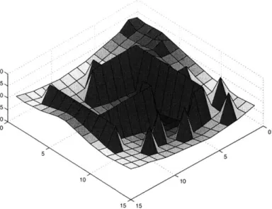
The Fast Marching Method is part of the Theory of Curve and Surface Evolution developed recently by J.A. Sethian [19]. The idea here is to simulate the propagation of a wave from the endpoint through the entire state space (the propagation speed depending on the cost of going from one point to another and ignoring reflection and dispersion effects) and to record the time T(x, y)' at which the wave pass at each point. These times T represent the shortest time (or length or smallest cost) to go from the endpoint to the particular point (x, y). T is a potential Field and a steepest gradient descent on it gives the shortest path to go to the chosen endpoint. Figure 3-3 shows a plot of this potential field on the same maze as in figure 3-1; it is easy to imagine how the wave has propagated from the target point, between obstacles, in the whole maze. By construction this field has only one minimum: the parent of a node has always a smallest value and only the endpoint has no parent (reminder: we assume that there is no negative cost).

This algorithm is based on the Eikonal Equation:

IV TI = F(x,y) where T is the time of arrival of the wave and F is the cost (or

the inverse of the celerity) at point (x,y).

The approach and the representation are very different from BFS and DP, but by looking into more details we can see that the simulation of the wave is done exactly in the same way : from the endpoint the algorithm measures the time to go to all neighbor points, then from all these new points, it looks one step further, finds the neighbors and calculates the time to go the next points. A good link between the two theories is to see the algorithm as an application of the Huygens principle in optic: at

200

110,

15 5

Figure 3-3: The potential field created by the artificial wave propagating in the maze. each step we consider the point being treated as a new light source (or wave source) propagating to its neighborhood.

3.3

Comparison

First of all it is interesting to note that virtually nobody mentioned that these tech-niques are so similar and that the structure of the computation done as an implemen-tation of those algorithms is the same. In each case, the computer will look almost

in the same order at the same points and their corresponding costs.

The main difference is the way intermediate results are stored during the process. In the BFS case the program stores for each vertices (or node or point explored) the parent it comes from, whereas in the two other algorithms, only the number of steps or the cost to go to this particular point is stored. This difference has three implications. First, a small advantage for BFS is that once you have gone through the whole graph, the time to explicitly output the shortest path is in o(1) at each step. For the DP and the FMM this time is in o(D) where D is the number of possible predecessors. But this is still very fast and it only represents a small fraction of the total cost, which comes from the backwards computation. Second, in BFS we said that the parent is stored for each vertices, that is a number between 0 and the total

number of parents, let's say o(nD) where D is the dimension of the graph and n is

the diameter of the graph. For the two other cases however only the number of steps

is stored, which is a number between 0 and the maximum length, o(n). The space

required to store a number is on the order of its logarithm, thus BFS requires D

times more memory space. However if the cost function is real instead of integer, the memory space needed to store the cost may become larger .

Dealing efficiently with small changes in the environment, like adding or removing an obstacle, points out another disadvantage of BFS. Indeed if only the parent and

not the cost is kept for each node, the whole graph has to be recomputed to take into account the cost change of an edge. For the two other methods it is very easy to correct the output when a cost is decreasing or when an obstacle is removed. In this case we just need to start a "wave propagation" from the point that has changed and update all following points that have then a lower cost than before.

Remark: The points that have been updated after an obstacle changed can be seen as the "shadow" of this obstacle. It is also the set of points whose shortest path to the goal goes through this point that has changed.

If the cost of an edge is increasing, or if an obstacle is added, the problem is much more complicated but still doable. The solution we propose is a bit tricky and consist first to simulate a very small cost decrease of the edge that is changing and apply the previous algorithm to find all the points that depend on the changed point (this is its "shadow"). We know that only the points in the shadow domain might need to

be updated. Thus we just need to put all the points on the border2 _{of the shadow in}

a sorted queue and do the wave propagation algorithm from here, on the shadow. Of course every new point found has to be inserted according to its cost in the ordered queue. In a word, if the intermediary costs are stored, it is easy and fast to correct them after a small change in the environment.

Last but not least with the DP and FMM, we keep more information in memory during the backwards computation, which can be used during the forward process, when making the path explicit. At each state we can find out all the controls that will lead to a path of shortest distance, whereas in BFS only one parent (which is now a child in the forward process) was stored. Thus it is easy to build a forward tree containing all possible shortest paths and choose between them:

- _{according to another constraint ;}

- by going through some interesting points;

- by choosing compliant trajectories of N different robots in the same environment

(this is faster than the exact solution using a 2N dimensional problem ).

Another similar problem, which is easily solved with FMM is the cat-mouse prob-lem where the cat has to plan a trajectory to intercept the mouse, which follows a known trajectory. Just simulates a wave from the current position of the cat. This will give us a sort of cone (a surface similar to figure 3-3 for which the z coordinate correspond to the lowest time t needed to go to the corresponding (x,y) point). The trajectory of the mouse is an increasing line in this (x,y,t) space. Where they intersect is the target where the cat has to go to catch the mouse.

3.4

Improvement

The cost of the previous algorithms depends on two main factors: the size or diameter of the problem and its dimension. The dimension has an exponential effect on the

2

More precisely, the border is the set of points that are not in the shadow domain but are connected to a point in the shadow domain

R

Figure 3-4: The stripped region represent the points explored at the time the algo-rithm stops, when using two waves (2D case). This has to be compared to the area of the big circle, corresponding to one wave.

computational cost, but this is also the reason why the following improvement can be significant.

If the goal is to find only one shortest path and find it as fast as possible, the algorithm will stop as soon as it finds one. But in this case the algorithm can be significantly improved by considering two waves propagating, one from the starting point and one from the target point. The algorithm will stop as soon as the two waves meet. To quantify the gain in computational time, we will suppose that our state space is like the usual Cartesian space. Thus in the usual case (one wave), the number of point explored is in the order of the volume of a ball of radius r, whereas in the second case, it is in the order of the volume of two balls of radius r/2. Looking at figure (3-4) makes it easier to understand; in short, in the first case, the time is

o(rD) and in the second case, o(2(r/2)D) : the gain is 2D-1, where D is the dimension

of the state space.

It has been verified on simulations that in the 2D maze problem, the program runs about twice as fast and in the dynamic problem (4D), it is possible to find the

shortest path more than eight times faster3. If the problem would be to navigate in

a 3D maze, typically the robot arm avoiding natural obstacles, we would have a 6D state space and the gain using two waves would be up to 26-1= 32 times faster. This can make a real difference when implementing a control in real time.

The gain of using two waves is the most important on problems where the

com-plexity comes from a large dimension instead of a large diameter4 of the state space.

To verify this assumption, an algorithm to solve the Traveling Salesman Problem has been implemented.

3

Since the maze is not a perfect Cartesian space, the gain depends actually on the configuration and the choice of the initial and target points and can vary from 0 up to 10.

4