HAL Id: hal-02643261
https://hal-agroparistech.archives-ouvertes.fr/hal-02643261v2
Submitted on 30 May 2016
HAL is a multi-disciplinary open access archive for the deposit and dissemination of
sci-L’archive ouverte pluridisciplinaire HAL, est destinée au dépôt et à la diffusion de documents
To cite this version:
Elodie Rouvière, Raphael Soubeyran. Competition vs. quality in an industry with imperfect trace-ability. Economics Bulletin, Economics Bulletin, 2011, 31 (4), pp.3052-3067. �hal-02643261v2�
Volume 31, Issue 4
Competition vs. quality in an industry with imperfect traceability.
Elodie Rouviere
AgroParisTech
Raphael Soubeyran
INRA, UMR1135 LAMETA, F-34000 Montpellier, France.
Abstract
We consider an industry where firms produce goods that have different quality levels but firms cannot differentiate themselves from rivals. In this situation, producing low-quality generates a negative externality on the whole industry. This is particularly true when consumers cannot identify producers. In this article, we show that under a "Laissez Faire" situation free entry is not socially optimal and we argue that the imposition of a Minimum Quality Standard (MQS) may induce firms to enter the market.
1
Introduction
There exist situations where products are not traceable by consumers and con-sumers are not able to identify either the producer or the level of quality of prod-ucts or services. When doing their choices, consumers mainly base their decisions on the reputation of the entire industry. In this sense, …rms share, at least par-tially, the reputation of the industry. An empirical evidence for this phenomena is food safety. Food safety is a credence attribute of product: consumers are not able, because it is too costly, to check the real quality of the product even after consumption. Even if products may have di¤erent safety levels, consumers con-sider products as generic (e.g fresh produce). Indeed, after an outbreak of food poisoning, everyone in the industry will su¤er from the safety outbreak. Since mid-may, the “E-coli cumcumber outbreak”has killed 16 people and infects more that 1100 people in Europe. The Spanish Federation of Producers / exporters (FEPEX) estimates lost sales up to e200 million per week. The cucumber crisis has also a¤ected French producers, who, according to the tomatoes and cucumbers producers association su¤er from a fall of sales of French cucumbers by 75%.1
In this article, we address the issue of entry in an industry where …rms pro-duce di¤erent quality levels but cannot di¤erentiate themselves from their rivals. Also, producing low-quality generates a negative externality on the whole indus-try. We build a simple model and we show that the link between market structure and welfare is ambiguous. In the “Laissez Faire” situation, an increase in the number of …rms has two opposite e¤ects. First, it leads the price to decrease increasing welfare. Second, incentives to free ride increase, reducing the average level of quality and then reducing welfare. Free entry is thus not socially optimal. Contrarily to conventional wisdom, we argue that the imposition of a Minimum Quality Standard may induce …rms to enter the market and increase welfare.
We have in mind the safety issue of fresh fruit and vegetables in Europe which is one-dimensional, as opposed to the United States where regulation on the safety of those produce also refers to the presence of microbiological hazards such as E-coli, Salmonella, etc. The de…nition of food safety for fresh fruit and vegetables in Europe relies on the Maximum Residue Limits for pesticides (MRLs) set by the European authorities (Regulation (EC) No 396/2005). Residues found in or on produce are judged, according to these laws, as being above, at or below the limit. Any food operator must comply with a “performance standard”, as de…ned in Henson and Caswell (1999): the food product they market should reach the prescribed product quality standards and/or safety levels. How they do reach the standard is left to the discretion of the food operators. Public agencies in charge of enforcing law and monitoring food safety, mostly conduct regular on-site and
product-oriented inspections. In the case of fresh produce, samples are collected and laboratory analyses are carried out to check that residue levels are within the legal limits (see for instance Rouvière et al. 2010). If excess levels are found, food operators are found guilty of an o¤ence and the whole box of the incriminated product is taken o¤ the market. The cost of conducting a laboratory analysis (e300 in average) prevents from analyses conducted by consumers.
The closest literature on this issue is the literature about collective reputa-tion. Tirole (1996) considers that collective reputation should be assumed to be the aggregate reputation of individual agents. In a context of imperfect informa-tion available to consumers about quality, he shows that the composiinforma-tion of the producer group matters. Winfree and McCluskey (2005) assume that collective reputation is a common property resource and show that the (exogenous) number of …rms should be considered closely because of free-rider e¤ects. However, in those studies, the size of the group of producers is taken as …xed and then does not allow for entry in or exit from the group. Our model, although static, endogeneizes the entry decision.
Moreover, our article directly participates to the controversial debate in the industrial organisation literature as regards to the e¤ect of a Minimum Quality Standard (MQS) on competition (for instance, see Leland 1979). Ronnen (1991) shows that an adequate MQS can increase both quantities sold and quality and then social welfare. The intuition of this result is that an increase in the low quality induces an increase of the high quality (in order to soften price competition) but equilibrium prices are however lower and more consumers buy the product (see also Crampes and Hollander 1995 for a similar result). The robustness of this result has been questioned in few direction. Valetti (2000) shows that this statement is sensitive to the mode of competition and Scarpa (1998) shows that it depends on the duopolistic market structure. Garella and Petrakis (2008) justify the use of MQS in industries where consumers face imperfect information. They point out that a MQS will change the consumers’perception on quality. However, none of these papers consider the possibility of entry and/or exit. As Boccard and Wauthy (2005) have already underlined, studying quality regulation through quantity regulation, MQS would induce …rm to exit the market and/or reduce the entry of new …rms. Our model of quality di¤ers from previous studies because there is no di¤erentiation but quality externalities.
The article proceeds as follows. We set up the theoretical model to emphasize the free entry issue in a “Laissez Faire”situation. Next, we analyse the competition e¤ect when a MQS is imposed on the industry. Finally, we provide our conclusions and their policy implications.
2
The Model
We focus on an industry in which identical and risk neutral …rms choose their level of quality in order to avoid quality failures. Products may have di¤erent quality levels but quality is a credence attribute: consumers are not able to observe these di¤erent quality levels even after consumption. Then, consumers only rely on the reputation of the entire industry.
Because we consider a static framework where the reputation of the industry depends on the produced levels of quality, we don’t rely on the past history of the industry. The model can thus be interpreted as an investigation of the reputational problem faced by an infant industry.
We consider a two-stage game. In the …rst stage, pro…t maximising …rms choose whether or not to enter the market. If a …rm enters the market, it faces a …xed (sunk) cost F > 0. Since we focus on quality, each …rm produces one unit of the product. In the second stage, the …rm chooses a quality level si 0 with cost
C (si)where C0 > 0and C00 > 0. We assume that the reputation of the industry is
“good”with a probability R (sa)that only depends on the average level of quality
(for simplicity) which is given by sa with
sa =
P
i2N
si
n (1)
where N denotes the set of the n …rms which enter the market, with R0 > 0 and
R00 0. The industry reputation is “bad”with probability 1 R (s
a). The inverse
demand function is then P (n) (with P0 < 0) if the reputation of the industry is
“good”, and the inverse demand function is 0 if the reputation of the industry is “bad”2. Therefore, the expected pro…t of …rm i is
i = R (sa) P (n) C (si) F; (2)
We make the following assumptions on the pro…t function which hold all through the paper.
Assumption 1: The pro…t of a monopolistic …rm is non negative when its quality level is optimal,
F R (sM) P (1) C (sM) ; (3)
2This is simply a normalisation. Indeed, suppose that if the reputation is "bad", the
in-verse demand drops to P (n) with 0 < 1. The expected inverse demand is R (sa) P (n) +
(1 R (sa)) P (n). It can be rewritten as (R (sa) + (1 R (sa)) ) P (n). To see that our
where sM denotes the optimal quality e¤ort of the monopolistic …rm, i.e.
sM = arg maxfR (s) PM C (s) ; s 0g : (4)
Assumption 2: A monopolistic …rm’s pro…t is non positive when its quality level is large enough,
lim
s!+1(R (s) P (1) C (s) F ) 0: (5)
In our setting, we can apply the result provided in Spence (1975) (see propo-sition). The (expected) inverse demand function is R(s)P (n) and we have
@2(R(s)P (n))=@s@n < 0; (6)
thus the monopoly always undersupplies quality (as with consumers’preferences à la Mussa-Rosen (Mussa and Rosen, 1978)). In other words, the monopoly will always underinvest in quality because of the distortions that exist between …rms and the society. Our model di¤ers from those seminal works since we focus on an oligopoly where quality externality among …rms induces a second and new distortion.
3
“Laissez faire” situation
In this section, we solve the game described above where there is no intervention from the regulator. We solve the game through backward induction.
First, we solve the second stage of the game. Assume that n identical …rms entered the market in the …rst stage. Firms individually make their quality choice, si. The optimisation problem for …rm i is then
M ax
si 0
(R (sa) P (n) C (si)) ; (7)
The …rst order condition is 1 nR
0(s
a) P (n) = C0(si) : (8)
This condition allows to de…ne …rm i0s best response as an implicit function of the
average quality sa (and of the number of …rms n) as usual in “private provision
of a public good” games. Note that @si
@sa = 1
nR00(sa)P (n)
C00(si) 0. Hence, as the average
quality sa increases, …rm i has an incentive to decrease its quality level.
In an interior equilibrium, the …rms’ quality levels are identical (due to the convex nature of the cost function C), i.e. for all i, si = s which is characterised
by:
1 nR
0(s ) P (n) = C0(s ) : (9)
This equilibrium condition implicitly de…nes the equilibrium quality level, s , as a function of the number of …rms n.
Proposition 1 An increase in the number of …rms lowers the equilibrium quality level, dsdn < 0.
When the number of …rms increases …rms have incentives to decrease their quality level. First, quality e¤orts are diluted in the industry reputation then …rms’ incentives to free ride increase (this results is similar to Winfree and McCluskey (2005)). Second, the price of the product decreases. Each …rm’s expected bene…ts decrease then …rms provide a lower quality level.
Second, we derive the subgame perfect equilibrium of the game. In the …rst stage, …rms anticipate the equilibrium quality level (characterised at stage 2) and decide to enter the market if their ex-ante expected pro…t is non negative. The number of …rms who enter the market n is then characterised by:
R (s (n )) P (n ) C (s (n )) = F; (10)
where n ( 1 according to Assumption 1) denotes the equilibrium number of
…rms which is an implicit function of F , the sunk cost of entry. Di¤erentiating condition (10) with respect to F we obtain:
dn dF = [R 0(s ) P (n ) C0(s )]ds dn + R (s ) P 0(n ) 1 : (11)
From condition (9), we obtain
R0(s ) P (n ) C0(s ) = (n 1) C0(s ) 0 (12)
When a …rm decides to enter the market, it anticipates that the price (P0(n ) < 0)
and the equilibrium quality will decrease (dsdn < 0). Consequently, the number of …rms increases only if the entry cost decreases:
dn
dF < 0: (13)
This result strongly depends on the fact that the number of …rms has a negative impact on the equilibrium quality.
Welfare e¤ect of the market structure: In order to appraise the welfare e¤ect, we consider the equilibrium quality game (stage 2), where each …rm provides the
same (second stage equilibrium) quality level s (n) de…ned by condition (9), with
1 n n . We focus on the e¤ect of an increase in the number of …rms on
consumer surplus and on social welfare.
Consumer Surplus: Under the assumption of quasi-linear consumer utility,
when there are n …rms, the expected (Marshalian) consumer surplus is
CS (s ; n) = R (s ) 2 4 n Z 0 P (z) dz P (n) n 3 5 : (14)
The marginal e¤ect of an increase in the number of …rms on the expected consumer surplus is dCS dn = @CS @n + @CS @s ds dn: (15)
The direct e¤ect is given by @CS
@n = R (s ) [ P
0(n) n] > 0; (16)
i.e. consumer surplus increases through a decrease in the price of the product. The indirect e¤ect, @CS@s dsdn, represents the e¤ect of an increase in the number of …rms through its impact on the equilibrium quality. We know from Proposition 1 that dsdn < 0. The e¤ect of an increase of the quality level on consumer surplus is given by @CS @s = R 0(s ) 2 4 n Z 0 P (z) dz P (n) n 3 5 > 0: (17)
Then, @CS@s dsdn < 0, i.e. the indirect e¤ect is negative. Finally, the global e¤ect of an increase of the number of …rms on consumer surplus is ambiguous because both the price and the quality of the product decrease.
Social Welfare: Social welfare is denoted by W = W (s ; n), with W (s ; n) given by: W (s ; n) = R (s ) n Z 0 P (z) dz n [C (s ) + F ] ; (18)
We now evaluate the welfare e¤ect of competition. Di¤erentiating condition (18) with respect to n, we obtain
dW dn = @W @n + @W @s ds dn: (19)
The welfare e¤ect is twofold. The direct e¤ect is given by @W
@n = R(s )P (n) [C(s ) + F ] : (20)
As long as pro…ts remain non negative, @W
@n has a positive value. This represents
the classical positive e¤ect of competition. The indirect e¤ect is given by @W@s dsdn. According to Proposition 1, the quality level decreases with respect to the number of …rms, ds
dn < 0.
The welfare e¤ect of an increase in the quality level is given by @W @s = R 0(s ) n Z 0 P (z) dz n C0(s ) : (21) Since P0 < 0, we have P (n ) < n Z 0 P (z) dz: (22)
According to the latter condition and (9) @W
@s has a positive value. Therefore,
the indirect welfare e¤ect, @W@s dsdn, has a negative value. The welfare e¤ect of competition is ambiguous. An increase in the number of …rms reduces each …rm’s market power and prices, thereby improving social welfare. Yet at the same time, it lowers the average quality, reducing social welfare.
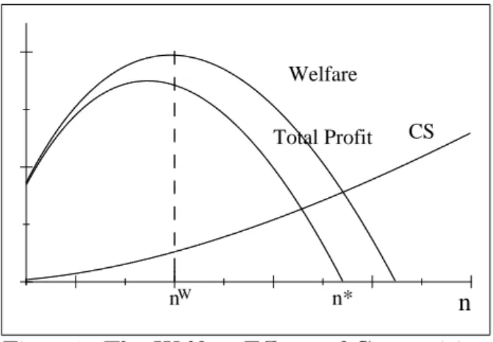
Proposition 2 Under the “Laissez Faire” situation, at the free entry point the number of …rms is larger than the optimal number of …rms.3
Proposition 2 states that n > nW,4 where nW represents the number of …rms
that maximizes social welfare. Figure 1 illustrates this result.5
3Until now we have ignored the integer problem. Our results are qualitatively una¤ected if
we consider n as an integer (the mathematical writing is a bit di¤erent).
4Considering n has an integer, this inequality would be weak. Indeed, in the space of real
numbers, the welfare function may have an optimum reached between two integers and the free entry point may also be between these two integers. In this case, the welfare optimal integer level is the free entry integer number of …rms.
5Figure 1 represents the following speci…cation of the model. The industry reputation is
characterized by a logit function of the average quality, sa: R (sa) = 1+ssaa. The inverse demand
function is assumed to be linear, P (n) = n where > 1. The cost function is C (si) = 1
2(1 + si) 2
n n* nW Total Profit Welfare CS
Figure1. The Welfare E¤ects of Competition
Figure 1 also illustrate the welfare e¤ect of competition. Welfare …rst increases and then decreases with the number of …rms. When n …rms compete in the market under the “Laissez Faire” situation, the positive welfare e¤ect of competition is lower than the negative e¤ect of free-riding on quality. Therefore, the regulator needs to intervene in order to avoid free-riding incentives and to prevent the entire industry from failing to perform. This result contributes to the critical debate in the industrial organisation literature that concerns the justi…cation of anti-competitive regulation. For instance, Mankiw and Whinston (1986) have shown that in homogeneous product markets, free entry can lead to a socially excessive number of …rms. They model a situation in which the output per …rm falls as the number of …rms in the industry increases. In our model, we assume that the output per …rm is constant, however, the free-riding incentives lead us to the same conclusion.
4
Minimum Quality Standard
In this section, while maintaining our focus on the entry issue, we examine the situation where the regulator imposes a Minimum Quality Standard (MQS). We assume that, before stage 1, a MQS s is announced. Firms decide to enter the market at stage 1 and choose a quality level si sat stage 2. Since the purpose of
this section is to compare the e¤ect of di¤erent levels of MQS, we do not consider the regulator as a player, that is s is given.
Market structure and MQS: In this section, we derive the equilibrium of the
game for di¤erent levels of the MQS, s 0. The equilibrium quality and the
equilibrium number of …rms will depend on the level of the MQS. Let us
de-note s = s (s; n) the equilibrium quality of stage 2 and n = n (s; F ) the
equilibrium of this game under the “Laissez Faire” situation, that is for s = 0. In other words, s (0; n) and n (0; F ) are such that s (0; n) = s (n) and n (0; F ) = n (F ), where s characterised by condition (9) and n characterised by condition (10).
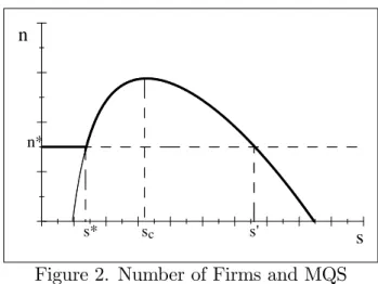
In order to present the next proposition, we need to de…ne a particular quality level and a particular number of …rms denoted by scand nc, respectively. scand nc
are de…ned as the equilibrium quality level and the equilibrium number of …rms of the following two stage game: at stage 1, …rms enter the market if their expected pro…t is non negative, and at stage 2 …rms behave cooperatively, i.e. each …rm provides the same quality level in order to maximise the total pro…t of the industry, n (R (s) P (n) C (s)). sc and nc are characterised by R0(sc) P (nc) = C0(sc)and
R (sc) P (nc) C (sc) F = 0.
Proposition 3 There exists a unique symmetric equilibrium and,
(i) If s s ; then the MQS has no e¤ect on quality, i.e. s = s , neither on
competition , i.e. n = n ,
(ii) If s < s, then the MQS is binding s = s. There exists s0 s
c such that for
s s s0, n n and for s0 < s, n < n . The maximal number of …rms is
nc and is achieved for s = sc.
Relatively to the “Laissez Faire”situation: If the MQS is not binding (s s ), the MQS does not alter either competition or the …rm’s quality level.
We discuss now the case when the MQS is binding: Increasing the level of the MQS (s < s < sc) increases the level of the industry reputation by increasing
…rms’ quality levels. The MQS induces …rms to enter the market as long as the cost of providing the MQS level is su¢ ciently low. When the MQS equals to the cooperative equilibrium quality level (s = sc), the industry reputation is
maxi-mal. When the MQS is imposed at such a level, a maximum number of …rms (nc)
enters the market. For MQS levels which are higher than the cooperative equi-librium quality level (s > sc), the marginal cost of providing quality overcomes
the marginal bene…t that leads to a drop in pro…ts. However, the number of …rms remains higher than it would be under the “Laissez Faire”situation as long as the MQS is low enough (sc< s s0). For the highest MQS levels (s0 > s), the number
of …rms becomes lower than the number of …rms in the “Laissez Faire” situation (n ). This is the only situation in which the MQS can reduce competition. Figure 2 illustrates those results.
s n
s* sc s'
n*
Figure 2. Number of Firms and MQS
In the light of these statements, we turn now to analyse the welfare e¤ect after the introduction of a given MQS.
Welfare e¤ect of the MQS: When a MQS s is imposed, the social welfare
function can be written as
W (s ; n ) = R(s ) 2 4 nZ 0 P (z)dz n P (n ) 3 5 : (23)
According to the result of Proposition 3, we can provide the following relationship between the level of the MQS and social welfare:
Corollary 4 Relatively to the “Laissez Faire” situation, social welfare is (i) un-a¤ected when the level of the MQS is su¢ ciently low (s s ), (ii) improved when the level of the MQS is in a middle range (s < s s0).
Relatively to the “Laissez Faire” situation, the introduction of a MQS unam-biguously improves welfare as long as the level of the MQS leads to a greater number of active …rms.
5
Conclusion
We have considered industries where …rms provide di¤erent quality levels. They cannot di¤erentiate themselves from their rivals but can su¤er from externalities due to rivals low-quality levels. We have shown that a “Laissez Faire” situation leads to a sub-optimal number of …rms in the market. The regulator face di¤erent solutions which all have their positive and negative e¤ects both on quality and competition. In such a case, the regulator face a trade-o¤ between quality and
competition. The regulator can choose to restrict the number of …rms in the market. On the one hand, such regulation would limit the incentive to free ride and then provide a su¢ cient level of quality. On the other hand, this regulation has also two negative e¤ects. First, it leads to an increase in the price. Second, free riding incentives are reduced but they are not eradicated. The other solution available is the introduction of a Minimum Quality Standard. We have shown that a Minimum Quality Standard can eradicate incentives to free-ride and can sustain both a high average level of quality and a high degree of competition.
Appendix
Proof of Proposition 1
Di¤erentiating condition (9) with respect to n we obtain ds dn = 1 nP 0(n) + 1 n2P (n) R0(s ) 1 nR00(s ) P (n) C00(s ) ; (24) Since P0 < 0, we have 0 < 1 nP0(n) + 1 n2P (n) . Moreover, R0(s ) > 0, then, sign ds dn = sign 1 nR 00(s ) P (n) C00(s ) < 0: (25)
Proof of Proposition 2
We evaluate the marginal variation of welfare at the free entry point. Di¤erenti-ating condition (18) with respect to the number of …rms n; we obtain
dW dn (s ; n ) = 2 4R0(s ) n Z 0 P (z) dz n C0(s ) 3 5@s @n (26)
According to Proposition 1 and @W @s = R 0(s ) n Z 0 P (z) dz n C0(s ) > 0; (27)
This expression has a strict negative value.
Proof of Proposition 3
When the MQS is not binding, i.e s s , it is straightforward that s = s and
n = n .
When the MQS is such that s > s , it is straightforward that s = s. Consid-ering the number of …rms which enter the market at stage 1, n , is characterised by
Di¤erentiating this condition with respect to s leads to @n @s = R0(s) P (n ) C0(s) R (s) P0(n ) ; (29) Then, sign @n @s = sign [R 0(s) P (n ) C0(s)] : (30)
R (s) P (n ) C (s) is the per …rm pro…t when all the quality levels are s. Per …rm pro…t is increasing for s scand decreasing for sc s. Hence, @n@s 0when
s sc and @n@s 0 when sc s. Then, n achieves its maximum, nc for s = sc.
Moreover, according to Assumption 2, lim
s!+1(R (s) P (1) C (s) F ) 0, then
lim
s!+1(n ) 1. Therefore, there exists s
0 s
c such that for s s s0, n n
and for s0 < s, n < n .
Proof of Corrolary 4
When the MQS is low, i.e. s s , according to Proposition 3, social welfare
is W (s ; n ) = W (s ; n ). When the MQS is in a middle range, s < s s0,
according to Proposition 3, social welfare is W (s ; n ) = W (s; n (s; F )) with s > s and n > n . Since social welfare unambiguously increases with respect to s and n , W (s ; n ) > W (s ; n ).
References
[1] Boccard, N. and X. Wauthy (2005) “Enforcing Domestic Quality Dominance through Quotas” Review of International Economics 13, 250-261.
[2] Calvin, L. (2007) “Outbreak Linked to Spinach Forces Reassessment of Food Safety Practices” Amber Waves 5(3), 24-31.
[3] Crampes, C. and A. Hollander (1995) “Duopoly and Quality Standards”Eu-ropean Economic Review 39, 71-82.
[4] Garella, P.G. and E. Petrakis (2008) “Minimum Quality Standards and Con-sumers’Information” Economic Theory 36, 283-302.
[5] Henson, S. J. and J. A. Caswell (1999) “Food Safety Regulation: an Overview of Contemporary Issues” Food Policy 24, 589-603.
[6] Leland, H. (1979) “Quacks, Lemons, and Licensing: a Theory of Minimum Quality Standards” Journal of Political Economy 87, 1328-1346.
[7] Mankiw, N.G. and M.D. Whinston (1986) “Free Entry and Social Ine¢ ciency” Rand Journal of Economics 17, 48-58.
[8] Mussa, M. and S. Rosen (1978) “Monopoly and Product Quality”Journal of Economic Theory 18, 301-317.
[9] Ronnen, U. (1991) “Minimum Quality Standards, Fixed Costs, and Compe-tition” Rand Journal of Economics 22, 490-504.
[10] Rouvière, E., Soubeyran, R., and C. Bignebat (2010) “Heterogenous E¤ort in Voluntary Programmes on Food Safety: Theory and Evidence from the French Import Industry of Fresh Produce” European Review of Agricultural Economics 37(4), 479-499.
[11] Scarpa, C. (1998) “Minimum Quality Standards with More than Two Firms” International Journal of Industrial Organization 16, 665-676.
[12] Spence, M.A. (1975) “Monopoly, Quality and Regulation” The Bell Journal of Economics 6(2), 417-429.
[13] Tirole, J. (1996) “A Theory of Collective Reputations (with applications to the persistence of corruption and to …rm quality)”Review of Economic Studies 63, 1-22.
[14] Valetti, T. (2000) “Minimum Quality Standards under Cournot Competition” Journal of Regulatory Economics 18, 235-245.
[15] Winfree, J.A. and , J.J. McCluskey (2005) “Collective Reputation and Qual-ity” American Journal of Agricultural Economics 87, 206-213.