Can eustatic charts go beyond first-order? Insights from the Permo-Triassic

Can eustatic charts go beyond first order? Insights from

the Permian–Triassic

B. Guillaume1_{, S. Pochat}2_{, J. Monteux}2,3_{, L. Husson}4_{, and G. Choblet}2

1_{UMR CNRS 6118, GÉOSCIENCES RENNES, OBSERVATOIRE DES SCIENCES DE L’UNIVERS DE RENNES (OSUR), UNIVERSITÉ DE RENNES 1, 35042 RENNES CEDEX, FRANCE}

2_{LABORATOIRE DE PLANÉTOLOGIE ET GÉODYNAMIQUE, UNIVERSITÉ DE NANTES–CENTRE NATIONAL DE LA RECHERCHE SCIENTIFIQUE (CNRS), UMR-6112, 2, RUE DE LA HOUSSINIÈRE,} 44322 NANTES CEDEX 03, FRANCE

3_{LABORATOIRE MAGMAS ET VOLCANS, UMR 6524, 6 AVENUE BLAISE PASCAL, 63178 AUBIÈRE CEDEX, FRANCE}

4_{ISTERRE, CENTRE NATIONAL DE LA RECHERCHE SCIENTIFIQUE (CNRS), UNIVERSITÉ GRENOBLE ALPES, 38000 GRENOBLE, FRANCE}

ABSTRACT

First-order variations of eustatic charts (200–400 m.y.) are in agreement with our understanding of the geodynamic processes that control sea level. By extrapolation, second-order (10–100 m.y.) and third-order (1–10 m.y.) variations are also thought to follow the same rules. However, this assumption may be jeopardized by a closer examination of the Permian–Triassic example, for which climatic and tectonic eustasy fails to explain the variations of the eustatic charts. During this period, eustatic charts peak down to their lowermost Phanerozoic values and display second-order variations at rates of up to 3 m/m.y., which is inconsistent with the expected eustatic signal during the early fragmentation of the Pangean supercontinent and the late Paleozoic melting of ice sheets. Here, we review the possible mechanisms that could explain the apparent sea-level variations. Some of them do modify the eustatic sea level (ESL). In particular, dynamic deflections of Earth’s surface above subduction zones and their locations with respect to continents appear to have been the primary controls of absolute sea level as the Pangean supercontinent formed and broke up. Other mechanisms instead only locally or regionally produced vertical ground motions, either uplifting continents or tilting the margins where the control points were located. We show that (1) the thermal uplift associated with supercontinent insulation and (2) the dynamic uplift associated with the emplacement of a superplume both give rates of sea-level change in the range of long-term changes of ESL. We also show that (3) the dynamic tilt of continental margins not only produces apparent sea-level changes, but it also modifies the absolute sea level, which in turn may end up in the paradoxical situation wherein fingerprints of ESL drop are found in the geological record during actual ESL rise. We conclude that second-order absolute sea-level changes may remain elusive for some time.

LITHOSPHERE; v. 8; no. 5; p. 505–518; GSA Data Repository Item 2016238 | Published online 30 August 2016 doi: 10.1130/L523.1

INTRODUCTION

Relative and Absolute Sea-Level Change

Eustasy, or absolute sea-level variations, corresponds to changes of the mean sea level with respect to a fixed reference frame (center of Earth, satellite). Such variations either result from a change in the volume of water in the oceans or from a change in the bulk volume of oceanic basins. Relative sea-level variations, measured as a change in shoreline elevation with respect to a continent, instead correspond to a combination of eustasy, vertical ground motion, and sediment supply. Both relative and absolute

sea-level variations respond to the joint effects of several mechanisms that act at a variety of space and time scales (for a review, see Conrad, 2013). Eustatic sea-level (ESL) charts are based on compilations of local measurements of relative sea level that are purportedly comprehensive enough to be representative. Eustatic charts are admittedly consistent to first order with our understanding of the geodynamic evolution of Earth, mostly following the cycles of continental aggregation and dispersal (e.g., Hays and Pitman, 1973; Kominz, 1984; Worsley et al., 1984; Husson, 2006; Müller et al., 2008; Spasojević and Gurnis, 2012; Conrad, 2013). However, second- and third-order cycles of eustatic charts are possibly more disputable, because of the entanglement of different processes that

act on both the volume of seawater and the shape of oceanic basins. For example, eustatic charts (Fig. 1; Vail et al., 1977; Hallam, 1992; Haq and Al-Qahtani, 2005; Miller et al., 2005; Haq and Schutter, 2008; Müller et al., 2008) show on average a global decrease of ~200 m between the Late Ordovician (ca. 450 Ma) and the Pennsylvanian (ca. 315 Ma), as well as an almost monotonous increase of similar amplitude between the Early Jurassic (ca. 195 Ma) and the Late Cretaceous (ca. 85 Ma). This long-term trend is consistent with the long-term evolution of the mean seafloor age and associated ridge volume (Fig. 1C; Conrad, 2013). In addition, climatic effects are likely responsible for higher-frequency variations during ice ages (around 440 Ma, 360 Ma, 300 Ma, or during the past 40 m.y.; Fig. 1D). Other aspects of eustatic charts, however, lack a clear correlation with tectonic and climatic eustasy. For example, the two distinct and successive apparent sea-level oscillations that occurred between the Pennsylvanian and the Late Triassic (Fig. 1B) are of note. These two highs share com-parable amplitudes (~60–100 m) and durations (~50–70 m.y.), with local maxima of sea level at ca. 215 Ma and ca. 300 Ma and a minimum at ca. 245 Ma. These two highs are even more distinct on the eustatic charts of Haq and Al-Qahtani (2005) and Haq and Schutter (2008), where they form twin peaks (Fig. 1A). In the next section, we focus on second-order sea-level variations, typically several tens of meters in magnitude and several tens of millions of years in duration. Focusing on these two cycles, we

show that these signals are generated by a combination of mechanisms, and that they may not only occur during these periods but at any time during the geological record.

As pointed out by Cloetingh and Haq (2015), sea-level charts include both eurybatic (regional) and eustatic (global) sea-level signals. We follow up on their approach and explore more specifically, on the basis of the Permian–Triassic example, the temporal resolution below which these charts could represent anything but eustasy to show that other processes likely dominate at shorter time scales than that of the assembly and dis-persal of a supercontinent (200–400 m.y.).

Permian–Triassic Climatic and Geodynamic Paradox

Tectono-Eustasy and Glacio-Eustasy

The Permian–Triassic interval coincides approximately with the life span of the supercontinent Pangea (320–185 Ma; Veevers, 2004), after its aggregation was essentially achieved, and before global dispersion was ubiquitous. For this reason, the global volume of mid-oceanic ridges is often considered as almost constant during this period, associated with a high mean age of the oceanic lithosphere (e.g., Cogné and Humler, 2008; Fig. 1C). This period should thus in principle coincide with per-sistent sea-level lows, unlike what eustatic charts suggest (Fig. 1B). In addition, the mismatch between the expected constant lowstand and the reported second-order sea-level variations is further challenged by the reconstruction of the oceanic lithosphere mean age based on the amount of continental fragmentation (Cogné and Humler, 2008), which suggested a local minimum in the rate of seafloor production at ca. 220–225 Ma, followed by a maximum at ca. 210–215 Ma. Such an evolution yields an ESL evolution that is not correlated with the 215 Ma sea-level high. Thus, tectono-eustasy obviously fails to explain the Permian–Triassic second-order oscillations of the eustatic chart (Fig. 1B).

Glacio-eustasy could possibly explain the discrepancy, because the late Paleozoic was a glacial period (Fig. 1D). Indeed, recent studies (e.g., Rygel et al., 2008; Isbell et al., 2012; Montañez and Poulsen, 2013; Fang et al., 2015; Beard et al., 2015) have provided the necessary resolution to appraise the dynamics of the late Paleozoic ice age (330–260 Ma; Fig. 1D). Between 325 Ma and 285 Ma, ice sheets extended over a large part of the Gondwana continent from the South Pole to a latitude of ~35°S. Ice sheets store seawater over continents, and the amount of free water in the oceans decreases by the same amount. The expected effect of such a glaciation is therefore a fast sea-level drop during the Pennsylvanian. During the Permian instead, climate shifted to hothouse conditions, and ice sheets melted until 260 Ma. Given the larger extent of the Carbonifer-ous ice caps compared to that of the Quaternary Last Glacial Maximum (LGM), ESL rise should have been as high as 200 m, which corresponds to the complete melting of ice since the LGM (130 m), along with the complete melting of the Greenland and Antarctic ice sheets (70 m; e.g.,

Alley et al., 2005). Overall, the expected evolution of glacio-eustasy for both the Pennsylvanian icing and Permian melting is at odds with, and even anticorrelated to, eustatic charts, which rules out glacio-eustasy as a primordial process during this period of time.

Tectono-eustasy and glacio-eustasy are the usual suspects for ESL change (Conrad, 2013), but their role may only hold at first order. Indeed, during the Permian–Triassic, their joint effects should have led to maximal ESL lows during the Early Permian. Instead, the specific evolution of ESL shows a general sea-level lowstand up to the Late Triassic punctuated by significant (~60–100 m) second-order sea-level variations (Fig. 1B). Alternative mechanisms need to be considered.

Alternative ESL Controls

Continental contraction associated with supercontinent aggregation could be invoked, because it contributes to an increase in the size of oceanic basins and thus a decrease in ESL. For instance, ~1000 km of

shortening along the ~2500-km-long Himalayan belt may have produced

a sea-level drop of ~20–30 m since 50 Ma (e.g., Conrad, 2013, and ref-erences therein). Conversely, continental rifting during Pangea breakup (180 Ma) contributed to ESL rise (between 20 m and 80 m; see Conrad, 2013), potentially counterbalancing the effects of contemporary orogenies. Minor and localized continental rifting occurred during the Pennsylva-nian–Early Permian (ca. 320–290 Ma) and during the Late Triassic (ca. 230 Ma), which modestly raised ESL (Gutiérrez-Alonso et al., 2008; Frizon de Lamotte et al., 2015). Although these phases of early rifting are temporally correlated with the two highs, the expected rate of ESL rise must be even lower than the values that are proposed for the main phase of Pangean breakup (ca. 180 Ma, 0.15–0.6 m/m.y.; Conrad, 2013) and thus could not match observed ESL variations for the two highs (typi-cally more than 1 m/m.y.).

Marine sedimentation could also modify ESL. During the Cenozoic, the sedimentary flux into the oceans may have contributed to a rise of 50–60 m in the sea level (Müller et al., 2008; Conrad, 2013). During the Permian–Triassic, the two highs (from 320 to 280 Ma and from 250 to 200 Ma) match peaks in the 87_Sr/86_{Sr ratio of the global ocean (from 325}

Ma to 300 Ma and from 250 to 200 Ma; Veizer et al., 1999; McArthur and Howarth, 2004; Kani et al., 2008), which is often taken as a proxy for the global sedimentary flux to the ocean and/or hydrothermalism (e.g., Korte et al., 2003; Allègre et al., 2010; Tripathy et al., 2012; Vollstaedt et al., 2014). The sedimentary flux peak from 325 to 300 Ma was the conse-quence of the Variscan collision, and the second 250–200 Ma peak was controlled by large-scale continental weathering during extreme climate conditions (Permian–Triassic event and Trias hothouse) and enhanced tectonic activity during Pangean climax (Pangea uplift, Cimmerian colli-sion, etc.; e.g., Veevers, 1994, 2004; Korte et al., 2003; Leeder, 2011; Song et al., 2015). Because the amplitude of the 87_Sr/86_{Sr peaks is of the same}

order as Cenozoic ones, the sedimentary flux during the Permian–Triassic

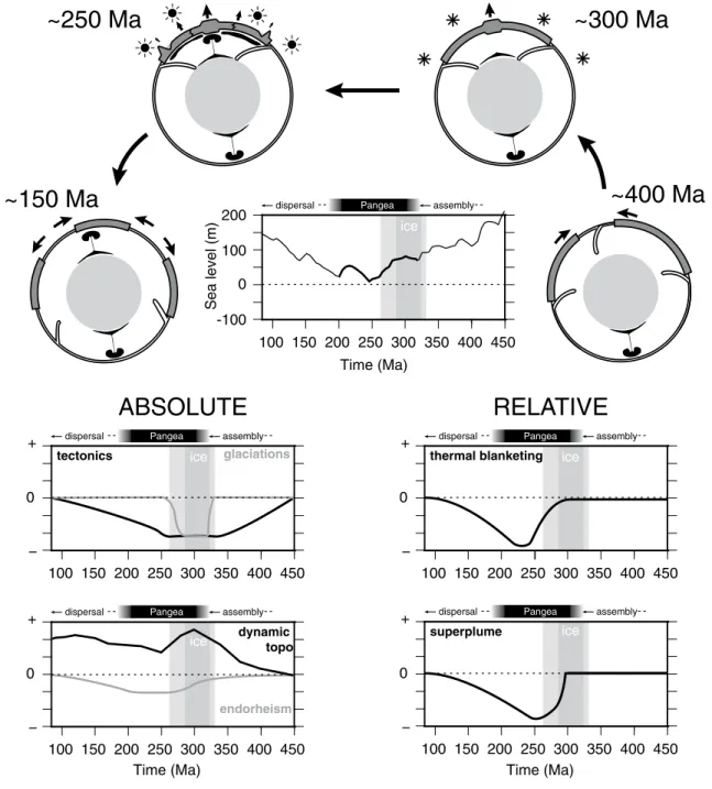
Figure 1. (A) Compilation of available sea-level curves for the last 550 m.y. (Vail et al., 1977; Hallam, 1992; Haq and Al-Qahtani, 2005; Miller et al., 2005; Haq and Schutter, 2008; Müller et al., 2008). (B) Averaged eustatic sea-level curve for the last 550 m.y. Gray envelope corresponds to the extrema. Second-order oscillations between the Pennsylvanian and the Late Triassic are shown as hatched. (C) Mean oceanic crustal age for the last 550 m.y. (Cogné et al., 2006; Müller et al., 2008; Spasojević and Gurnis, 2012; Müller et al., 2016; Cogné and Humler, 2008 [two curves]). (D) Main climatic events for the last 550 m.y. Periods of cool/cold climate are indicated in gray, and latitudinal ice extension is in blue (after Veevers, 1990; Golonka and Ford, 2000; Frakes et al., 2005; Vaughan, 2007; Fielding et al., 2008; Eyles, 2008; Isbell et al., 2012; Montañez and Poulsen, 2013; Brenchley et al., 2003; Caputo and Crowell, 1985). (E) Main tectonic events (after Raymo et al., 1988; Gregory-Wodzicki, 2000; von Raumer et al., 2003; Collins, 2003; Dickinson, 2004; Torsvik and Cocks, 2004; Veevers, 2004; Cawood, 2005; Cawood and Buchan, 2007; Windley et al., 2007; Gutiérrez-Alonso et al., 2008; Vaughan and Pankhurst, 2008; Wopfner and Jin, 2009; Wilmsen et al., 2009; Frisch et al., 2010; Nance et al., 2010; Bradley, 2011; Kroner and Romer, 2013; Torsvik and Cocks, 2013; Metcalfe, 2013; Stampfli et al., 2013; Veevers, 2013; Domeier and Torsvik, 2014). Blue and black bars correspond to oceanic domains and marginal orogenies and collisions, respectively. Neog.—Neogene.

40 50 30 60 0 20 40 60 80 100 120 140 160 180 200 220 240 260 280 300 320 340 360 380 400 420 440 460 480 500 520 540

C

Mean oceanic crustal age (Ma)

Cogné et al. (2006)

Cogné and Humler (2008)

Müller et al. (2008)

Müller et al. (2016)

Spasojevic and Gurnis (2012) 0 100 -100 200 0 100 -100 200 300 400 300 400 Cambrian Ordovician Silurian Devonian Carboniferous Permian Triassic Jurassic Cretaceous Paleogene Neog. 0 20 40 60 80 100 120 140 160 180 200 220 240 260 280 300 320 340 360 380 400 420 440 460 480 500 520 540

B

Pangea assembly dispersal Sea level (m) Miller et al. (2005)

Müller et al. (2008) Haq and Schutter (2008)

Haq and Al−Qahtani (2005) _{Vail et al. (1977)}

Hallam (1992)

Cenozoic Mesozoic Paleozoic

0 100 -100 200 0 100 -100 200 300 400 300 400 Cambrian Ordovician Silurian Devonian Carboniferous Permian Triassic Jurassic Cretaceous Paleogene Neog. 0 20 40 60 80 100 120 140 160 180 200 220 240 260 280 300 320 340 360 380 400 420 440 460 480 500 520 540

A

Pangea assembly dispersal Sea level (m) 0 20 40 60 80 100 120 140 160 180 200 220 240 260 280 300 320 340 360 380 400 420 440 460 480 500 520 540 40° 60° 80°

cold/cool period latitudinal ice extension

D

Latitud e ? ? Pacific Atlantic Indian Prototethys Gondwana Pangea margin Laramide/Sevier Andes Margin Orogenies Collision Oceanic domains Cadomian Caledonian

Himalayan/Alpine Cimmerian / Indosinian Alleghanian-Mauritanian-Ouachitan-Uralian-Variscan 0 20 40 60 80 100 120 140 160 180 200 220 240 260 280 300 320 340 360 380 400 420 440 460 480 500 520 540

E

Time (Ma) Paleopacific Panthalassa Rheic Iapetus Neotethys Paleotethys Figure 1.

peaks could have contributed to a comparable ESL rise of ~50–60 m. This reasoning holds with the premise that hydrothermalism remained constant throughout, and thus it remains highly arguable.

Temporal variations in the volume of volcanic material on the seafloor may contribute to sea-level change. Estimated rates of ESL Cretaceous rise and Cenozoic drop are as high as 1.5 m/m.y. and 0.5 m/m.y., respec-tively (Conrad, 2013). Estimating the contribution of volcanic material earlier than 150 Ma is virtually impossible because only a small fraction of seafloor of this age is still preserved, and we cannot exclude temporal variations in volcanic material during the Permian–Triassic, although we

cannot address this point.

Hydrated minerals in Earth’s mantle may store significant amounts of water (e.g., Hirschmann, 2006; Marty, 2012). Volcanic degassing and water-loaded subducting slabs into the mantle are sources and sinks of water and also modulate ESL (e.g., Korenaga, 2011; Crowley et al., 2011). However, we anticipate that their contribution scales with the time scale of mantle convection and supercontinental cycles. For instance, periods of continental dispersal are periods of younger seafloor and are associated with a larger flux of water out of the mantle and an ESL rise, whereas continental aggregation phases are associated with an ESL drop (Conrad, 2013). Such time scales are inappropriate to explain the Permian–Trias-sic ESL record.

Dynamic Topography and Thermal Blanketing

Other geodynamic processes associated with mantle convection dur-ing Pangean aggregation and fragmentation may provide robust alterna-tives to explain eustatic variations of sea level. Namely, we focus on dynamic topography and thermal blanketing. The amplitude of dynamic topography is as high as 1000 m, even at passive margins (e.g., Ricard et al., 1993; Steinberger, 2007; Moucha et al., 2008; Conrad and Hus-son, 2009; Guillaume et al., 2009; Braun, 2010), and its rate of change typically compares to eustatic variations. Its impact, when compared to the aforementioned processes that control eustasy, is partly regional and partly global. In other words, its effect on the relative sea level also has an absolute impact. Thermal blanketing underneath supercontinents (e.g., Gurnis, 1988; Coltice et al., 2007) also raises or lowers continental margins. Both mechanisms thus impact relative sea level at any place on Earth; however, ESL charts rely on sequence stratigraphy and subsid-ence curves from passive margins, which are implicitly considered stable because they are remotely located from tectonic plates boundaries. Last, secluding seawater in dynamically deflected basins modifies absolute sea level. Later herein, we investigate how these processes may have resulted in possible misconception and misinterpretation of both the observed low and the second-order variations in eustatic charts during the Permian–Tri-assic. Because these processes are often ignored, we take this example to dispute the significance of eustatic charts.

DYNAMIC TOPOGRAPHY ABOVE SUBDUCTION ZONES AND ABSOLUTE SEA-LEVEL CHANGE

Dynamic topography is the component of topography that is controlled by sublithospheric mantle convection. The viscous mantle flow deflects Earth’s surface by as much as ±1 km (e.g., Mitrovica, 1989; Ricard et al., 1993). Above subduction zones, in particular, the downgoing motion of a cold and relatively dense lithosphere within the mantle induces vertical stresses that contribute to several hundreds of meters of surface down-ward deflection (e.g., Mitrovica, 1989; Gurnis, 1992; Ricard et al., 1993; Husson and Guillaume, 2012).

Because dynamic topography lows at some place are on average com-pensated by highs elsewhere, it is therefore the distributions of continental

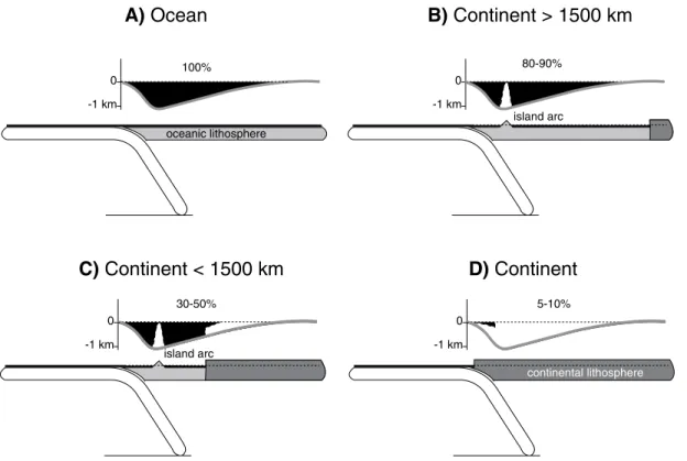
and oceanic areas over highs and lows in dynamic topography that impact ESL (Gurnis, 1992, 1993; Husson and Conrad, 2006; Conrad and Husson, 2009). In the case of intra-oceanic subduction, 100% of the negative deflec-tion converts into subsidence of the oceanic seafloor and contributes to an increase of oceanic basin volume, which in turn induces a drop in ESL. In the case of oceanic subduction underneath continents, only the fraction of the surface that is located at an elevation below the amplitude of the dynamic deflection will be flooded and contribute to the increase of oce-anic basin volume. An increase in the relative proportion of intra-oceoce-anic subduction zones with respect to subduction zones underneath continents thus results in an increase of the oceanic basin bulk volume and a drop of ESL. Of course, precisely quantifying the associated ESL variations requires a thorough knowledge of both the evolution of the downgoing lithospheres and the paleogeography and paleotopography of continents. One of the main challenges of such reconstructions is identifying intra-oceanic subduction zones in the past, as the geological archive gets sparse. Here, we apply a semiquantitative approach that aims at extracting the first-order trend of dynamic topography from the lengths of subduc-tion zones from paleotectonic maps (from Blakey, 2008). The lengths of subduction zones underneath oceans versus subduction zones under-neath continents can be considered as a first-order proxy for the relative contribution of dynamic topography for each type of subduction zone. However, many real-Earth cases do not fit in either of the plain intra-oceanic or beneath-continent subduction modes. A modern example is the Sumatra-Java subduction zone, where subduction occurs under emerged volcanic arcs with a back-arc sea that connects to the open ocean. In this case, dynamic subsidence drowns the oceanic floor and drops ESL, but it is locally not high enough to flood the volcanic arc. We therefore consider that at distances greater than 1500 km from the trench, the influence of dynamic topography is negligible (according to models; e.g., Husson, 2006). We distinguish four cases: (1) Subduction occurs under entirely flooded oceanic lithosphere, (2) the continent beyond the back-arc sea is at distances greater than 1500 km, (3) this distance is less than 1500 km, and (4) subduction occurs under almost unflooded continental litho-sphere (Fig. 2).

Figure 3 displays the length of the four categories of subduction zones measured at ~30 m.y. intervals for the last 450 m.y. Total subduction zone lengths measured from reconstructions by Blakey (2008) over the last 200 m.y. give an average value of 59,500 ± 8800 km, i.e., in the same range as the value found by Zahirovic et al. (2015) from paleomagnetic reconstructions (58,000 ± 5000 km). The total subduction zone length remains relatively constant for this period, whereas van der Meer et al. (2014) showed, on the basis of tomographic interpretation, a total subduc-tion length zone that was stable between 70,000 km and 80,000 km for the period 200–80 Ma (considering a slab sinking rate of 1.2 cm/yr) and then decreased to around 40,000 km at present day. The higher values found in this study may be attributed to the larger numbers of intra-oceanic subduction zones identified by seismic tomography. We tested its effect in our semiquantitative approach (Fig. 3). For previous periods (400–250 Ma), the mean total length is ~74,000 ± 7300 km, with a maximum at

340 Ma (~88,000 km), when intra-oceanic subduction zones were

virtu-ally inexistent. Of course, we cannot exclude the possibility that intra-oceanic subduction occurred at that time, but if it stayed at the same level as before the Carboniferous or after the Permian (i.e., around 30,000 km), it would raise the total subduction zone length to 118,000 km, which is almost twice as large as during the last 200 m.y. and seems very unlikely. General trends arise from this global picture: The aggregation of Pan-gea in the Carboniferous increased the subduction zone length under con-tinents and apparently decreased the length of intra-oceanic subduction zones. The Middle Permian to Late Triassic showed an approximately

twofold increase in subduction length underneath continents, which should have promoted ESL rise. However, at the same time, subduction underneath oceans also grew from almost zero at 280 Ma to a length of ~30,000 km at 220 Ma, which should instead have promoted ESL drop.

Therefore, the effects of each mode of subduction on the changes in ESL associated with dynamic topography must be taken into account. For this purpose, we define the index k:

k = –[(AL_o) + (BL_c>1500) + (CL_c<1500) + (DL_c)]/(L_o + L_c>1500 + L_c<1500 + L_c). Here, A, B, C, and D are coefficients that represent the proportion of dynamic topography that directly impacts the volume of oceanic basins

for subduction below oceans (length L_o), subduction below island arcs

with a continent farther than 1500 km (length L_c>1500), subduction below island arcs with a continent closer than 1500 km (length L_c<1500), and sub-duction below continents (length L_c), respectively (Fig. 2). The value of these coefficients and their evolution through time depend on the physical and kinematic properties of the subduction zones (e.g., slab dip, velocity, slab depth, age of the subducting oceanic floor, etc.), which are poorly resolved. We therefore grossly set these coefficients based on the dynamic topography model of Husson (2006). A was set to 1, as subduction occurs beneath oceans. For case B, we considered that island arcs are located ~200 km away from the trench and that the fraction of island arcs above

0 -1 km 100% 0 -1 km 5-10% 0 -1 km 30-50% 0 -1 km 80-90%

A) Ocean

B) Continent > 1500 km

C) Continent < 1500 km

D) Continent

oceanic lithosphere continental lithosphere island arc island arc

0

1

2

3

4

Length (1

0

4

km)

Car D S O Pe T J Cr Pa N A) ocean ice ice

0

1

2

3

0

1

2

3

B) continent > 1500 km C) continent < 1500 km

0

1

2

3

D) continent

0

100

200

300

400

Time (Ma)

modified with van der Meer (2014)

Pangea assembly

dispersal

Figure 2. Modes of subduction, as used to classify subduction zone lengths (Figs. 3 and 4). On top of each sketch, the gray line on the diagram rep-resents the theoretical dynamic subsidence above subduction zones. The part of this volume that is filled with seawater is represented in black (with the corresponding percentages), and the part occupied by solid Earth is in white.

Figure 3. Lengths of subduction zones during the last 450 m.y. for the four modes (see Fig. 2), as derived from the paleogeographic reconstruc-tions of Blakey (2008). For the top panel, we show an additional curve for the last 250 m.y. considering that the difference of total subduction zone lengths between our study and the study by van der Meer et al. (2014) corresponds to undocumented intra-oceanic subduction zones. Averaged eustatic sea-level curve from Figure 1B is also shown with a black dotted line; full time-scale labels are given in Figure 1.

sea level has a typical width of 100–200 km, similar to what is observed at present day in southeastern Asia for instance. The associated unflooded volume would represent 10%–20% of the total volume of subduction-induced dynamic subsidence computed from Husson (2006), and B was therefore set to 0.8–0.9. For case D, we considered continents that are ~100 km away from the trench to have a uniform mean elevation of ~875 m, similar to the current mean elevation of continents (e.g., Turcotte and Schubert, 2002). In this case, only 5% of the volume produced by dynamic subsidence would be occupied by oceans. Since continents close to active margins are lower than the mean elevation of continents, we considered a possible range for coefficient D between 0.05 and 0.1. Coefficient C is the most difficult to assess, since it depends not only on the physical and kinematic parameters of the subduction, but also on the distance between the trench and the closest continent, which varies in time and space. We chose intermediate values between B and D of 0.3–0.5 (for 875-m-high continents located 350 and 500 km away from the trench, respectively). Changing the values of these coefficients modifies the absolute value of k but not its relative evolution through time.

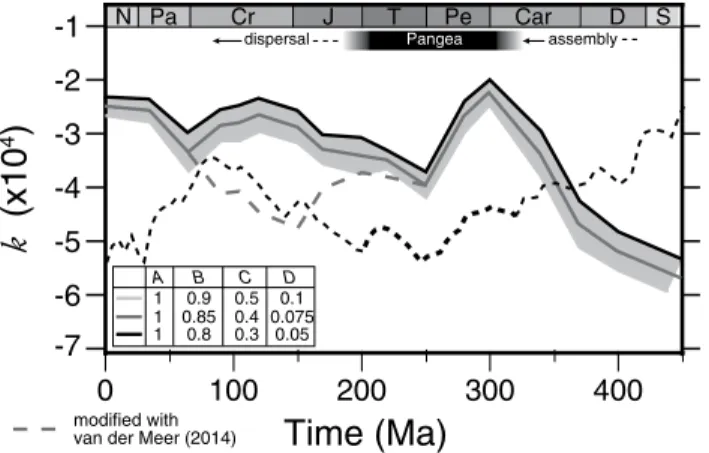
Time variations of k (Fig. 4) are indicative of the impact of dynamic topography on ESL. A rise in k means that the subduction length under-neath continents and arcs with neighboring continents increases with respect to subduction underneath oceans and remote continents. Also, a rise in k implies ESL rise. A drop of k indicates a drop in ESL. Last, k cor-relates with the first of the two highs of the eustatic charts, with an increase in k up to the very Early Permian and a low at the transition between the Permian and the Triassic Periods. In our model, k increases again at 250 Ma but does not display the expected decrease at the end of the Triassic. LOW SEA LEVEL OR HIGH CONTINENTS?

In the following, we explore the potentially important roles that dynamic topography and thermal blanketing played during Pangean

aggregation, during the Early Permian–Late Triassic time interval, by uplifting continental platforms and thus contributing to apparent—more than absolute—sea-level variations.

Thermal Blanketing

Supercontinental aggregation increases the sublithospheric mantle tem-perature by 100 K (Coltice et al., 2007; Phillips and Coltice, 2010) or even 300 K (Gurnis, 1988) without involving hot plumes; this process is known as thermal blanketing. It modifies the geotherm and in turn the crustal and lithospheric mantle density profiles. Next, we estimate the associated isostatic uplift during the 50 m.y. that followed the assembly of Pangea (ca. 320–270 Ma). In principle, this uplift can be investigated directly via convection models (see, e.g., the section “Supercontinent, Superplume, and Dynamic Topography”), which could include thermal blanketing, but in order to specifically isolate the respective impacts of dynamic uplift and thermal blanketing, we chose to treat them independently.

We consider a lithosphere of thickness d₁ ∈ (100, 200) km, which

includes a crust of thickness d_c = 30 km that is initially at conductive steady state. The radiogenic heating rate is 9 × 10-7 _W/m3 _{in the crust}

and zero below. Thermal conductivity is uniformly set to 3 W/m/K. Sur-face temperature is 300 K, and the initial temperature increase across the lithosphere is 1300 K. We then impose an arbitrary temperature increase ∆T ∈ (0, 300) K that mimics the thermal blanketing effect on the mantle,

and we monitor the conductive evolution of the lithosphere during 50 m.y. using a Crank-Nicholson method on a 100 cell grid mesh.

The density of crustal and mantle rocks was calculated following:

ρ•( )r = ρ − α0•[1 T r( )], (1)

with ρ0 corresponding either to the surface density of the crust (superscript

c, 2800 kg/m3_{) or density of the mantle at the Moho (superscript m, 3300}

kg/m3_{), and a being the thermal expansion coefficient (3 × 10}-5 _K-1_{). At}

each time step, the associated isostatic uplift h(t) for a compensation depth d₁ corresponding to the initial thickness of the lithosphere (Fig. 5A) is:

(

)

(

)

(

)

( )

( )

( )

( )

( )

( )

= ρ ρ + ρ ρ ρ h t ∆ d t d d t t 0 – – 0 – c c c l c m m m , (2)

where r•(t) is the average density of the crust or the mantle at time t. For an intermediate model with a temperature increase ∆T = 150 K at the base of a 150-km-thick lithosphere, the decrease in density reaches 0.5%. This translates to an isostatic uplift of ~200 m after 50 m.y. (Fig. 5).

-6

-7

-5

-4

-3

-2

-1

N Pa Cr J T Pe Car D S

k (x10

4

)

0

100

200

300

400

Time (Ma)

A 1 0.9B 0.5C 0.1D 1 0.85 0.4 0.075 1 0.8 0.3 0.05 modified with van der Meer (2014)

Pangea assembly dispersal Time (m.y.) Uplift (m ) 0 10 20 30 40 50 200 300 400 100 0 ∆T = 250 K ∆T = 150 K ∆T = 50 K

Figure 4. Variation of index k (see text) for different combinations of coef-ficients A, B, C, and D. These coefcoef-ficients correspond to the proportion of the dynamically subsided volume occupied by seawater (see Fig. 2) with

A—subduction under oceanic lithosphere, B—subduction zones with a

continent farther than 1500 km, C—subduction zones with a continent closer than 1500 km, D—subduction under continental lithosphere. Increas-ing k trends are indicative of increasIncreas-ing absolute sea level; conversely, decreasing k trends are compatible with decreasing sea level. Note k is also calculated by considering that the difference between our estimate of total subduction zone lengths and that of van der Meer et al. (2014) for the last 250 m.y. represents undocumented intra-oceanic subduction zones (gray dashed line). Averaged eustatic sea-level curve from Figure 1B is also shown with a black dotted line; full time-scale labels are given in Figure 1.

Figure 5. Time evolution of thermal uplift for a 150-km-thick lithosphere with different thermal anomalies at its base.

In detail, ~50% of this uplift is achieved within the first 15 m.y., which yields an average uplift rate of ~7 m/m.y. for this period. As expected, the temperature increase at the base of the lithosphere impacts the thermal uplift, and, for a higher-temperature anomaly of ∆T = 250 K, the thermal uplift is 325 m after 50 m.y. (Fig. 5). The uplift is almost insensitive to the initial thickness of the continental lithosphere, varying at most by

5% for the considered thickness d₁∈ (100, 200) km and ∆T ∈ (0, 300)

K ranges. Uplift rates are within the range of second-order variations in eustatic sea level. Because the entire supercontinent, including passive margins, has been affected by thermal blanketing, it would in turn have maintained an apparent eustatic low that is in fact a ubiquitous uplift of continental shorelines.

Supercontinent, Superplume, and Dynamic Topography

Superplumes are thought to arise during supercontinental aggregation (e.g., Li and Zhong, 2009) underneath supercontinents. These mantle upwellings, as opposed to downwellings in subduction zones, dynamically uplift the surface of Earth with amplitudes of several hundred meters, as illustrated, for instance, by the African superswell (e.g., Lithgow-Bertel-loni and Silver, 1998). Such an uplift directly impacts the elevation of the shorelines and may result in an apparent sea-level low.

Interestingly, the Permian Period recorded the emplacement of numer-ous large ignenumer-ous provinces (Fig. 6B), like the Siberian Traps (ca. 250 Ma; Renne and Basu, 1991; Renne, 1995; Reichow et al., 2009), the

elevation (297-284 Ma) _m -500 0 500 1000 1500 2000 elevation (151-145 Ma) _m -500 0 500 1000 1500 2000 elevation (255 Ma) m -500 0 500 1000 1500 2000 ° 0 6 − ° 0 6 − −30° −30° 0° 0° 30° 30° ° 0 6 ° 0 6 Basins (311-293 Ma): 1.1 x 107 _km2 Cordilleras (296-285 Ma): 1.6 x 107 _km2 Basins (256-245 Ma): 2.7 x 107 _km2 Cordilleras (269-248 Ma): 1.75 x 107 _km2 Basins (205-176 Ma): 3.1 x 107 _km2 Cordilleras (203-179 Ma): 6.8 x 106 _km2 ° 0 6 − ° 0 6 − −30° −30° 0° 0° 30° 30° ° 0 6 ° 0 6 ° 0 6 − ° 0 6 − −30° −30° 0° 0° 30° 30° ° 0 6 ° 0 6 ° 0 6 − ° 0 6 − −30° −30° 0° 0° 30° 30° ° 0 6 ° 0 6 ° 0 6 − ° 0 6 − −30° −30° 0° 0° 30° 30° ° 0 6 ° 0 6 ° 0 6 − ° 0 6 − −30° −30° 0° 0° 30° 30° ° 0 6 ° 0 6

A

B

C

Siberia Bachu Emeishan Oman Panjal W. Austr. Skagerrak

Pennsylvanian-Early Permian

Late Permian-Early Triassic

Late Triassic-Late Jurassic

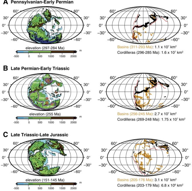
Figure 6. Paleotopography (left maps) (after Ziegler et al., 1997), and (right) shallow-marine shelf and undifferentiated ter-restrial depositional environment (orange; after Golonka and Ford, 2000), and areas of high elevation (>1 km, black) for (A) the Pennsylvanian–Early Permian, (B) the Late Permian, and (C) the Late Triassic to Late Jurassic. Note that time intervals slightly differ between left and right panels and are indicated below each map. For the Late Permian, the approximate areas of internal drainage are contoured by purple lines. The distribution of Middle-Late Permian large igneous provinces is also shown in red (after Isozaki, 2009), and the white stars represent the reconstructed position of the reference districts used by Haq and Schutter (2008) for the Late Permian.

Emeishan flood basalts (ca. 260 Ma; He et al., 2007, 2010; Sun et al., 2010; Shellnutt, 2014), the Bachu large igneous province (ca. 275 Ma; Zhang et al., 2008), and the Skagerrak-Centered large igneous province (ca. 300 Ma; Torsvik et al., 2008), which could have arose from a superplume that developed beneath the Pangean supercontinent (e.g., Isozaki, 2009). The emplacement times of these large igneous provinces all postdate Pangean aggregation by at least 20 m.y. and correspond to the period of reported low eustatic sea level. Dynamic uplift driven by mantle upwell-ings associated with the large igneous provinces should have affected the supercontinent, including its purported stable margins, which would have resulted in a relative sea-level drop. In the following, we numerically evaluate the dynamic uplift and relative sea-level drop associated with the upwelling of a thermal plume underneath a supercontinent. We do not investigate the origin of the superplume (which is debated elsewhere; see Li and Zhong, 2009; Condie et al., 2015), but only its effect on the vertical motion of Earth’s surface.

We follow the procedure adopted by Monteux et al. (2009, 2011, 2013;

see Data Repository1 _{for model setup). We monitor the dynamic}

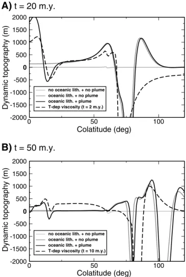
topogra-phy evolution during the thermo-mechanical readjustment as a function of the colatitude for t = 20 m.y. (Fig. 7, top panel) and t = 50 m.y. (Fig. 7, bottom panel). Figure 7 confirms that the presence of a large thermal

plume only weakly affects the behavior of the sinking slab. However, the ascension of the plume leads to a positive anomaly in the dynamic topography that scales to the size of the thermal plume. The amplitude

of this topographic anomaly can reach ~2000 m for the current modeled

thermal plume (Fig. 7, top panel) over a lateral extent of ~30°. Then, as the thermal plume is cooling, the radial velocity field vanishes below the supercontinent, and the dynamic topography decreases to values below 500 m, with a maximum at the edges of the plume (Fig. 7B, colatitudes 10°–15°). Maximum uplift rates originating from the plume rise are within the range 75–100 m/m.y., i.e., around one order of magnitude higher than those from thermal isostasy.

Of course our models do not capture the entire complexity of Pangean aggregation and breakup. Our simplistic models do not include litho-sphere dynamics that could affect the vertical motion of the margins and partially inhibit the observed dynamic uplift, nor the framework of the emergence of a superplume. Instead, these models should be envisioned as illustrative of the processes at play, with a quantification of the order of magnitude of the amplitude of dynamic topography. In our models, we assume a free-slip surface, and so the subduction is two-sided, and uplifts arise from either side of the circum-Pangea subduction zone (Fig. 7). In reality, the upper surface is free and deformable, which leads to single-sided subduction (e.g., Crameri et al., 2012). As the continental lithosphere is probably colder and drier than the mantle, it may lead to a viscosity contrast with its surrounding environment. To model this effect, we considered temperature-dependent viscosity (with a viscosity of the coldest material 100 times larger than the viscosity of the hottest mate-rial). Figure 7 shows that considering a temperature-dependent viscos-ity reduces the characteristic time scales for the spreading of the plume below the surface (Koch and Koch, 1995) and modifies the shape of the dynamic bulge. This generates a wider internal dome inside the super-continent and leads, after 10 m.y., to a global uplift of the super-continental lithosphere by ~300 m.

While these calculations involve a large-scale plume beneath Pangea, dynamic uplift caused by (smaller-scale) plumes might also occur in oceanic areas and thus contribute to sea-level variations. Indeed, oceanic

1 _{GSA Data Repository Item 2016238, details of numerical model methods and}

setup, is available at www .geosociety.org /pubs /ft2016.htm, or on request from editing@geosociety.org.

plateaus (region of thickened oceanic crust) are often considered to result from decompression melting of large mantle plume heads. Due to their increased thickness, oceanic plateaus are not easily subducted and are believed to often aggregate at continental margins (for a synthesis, see Kerr, 2014). A well-exposed example of such an accreted plateau is the Wrangellia terrane (Greene et al., 2010), which is believed to have formed 230–225 Ma in the Panthalassic ocean and later accreted (ca. 160–140 Ma) to western North America. Other candidates include the Cache Creek and Angayucham terranes, also in North America, as well as the Chichibu, Chogoku, and Mino-Tamba Belts in Japan (Kerr, 2014). A precise evalu-ation of the dynamic uplift associated with the emplacement of oceanic plateaus is controversial: The emblematic Ontong-Java Plateau was prob-ably much less uplifted than model predictions suggest (e.g., Kerr and Mahoney, 2007), while at least part of the volcanism associated with the formation of the Wrangellia terrane took place in a subaerial con-text, possibly indicative of at least some dynamic uplift. Similarly, the

-2000 -1500 -1000 -500 0 500 1000 1500 2000

no oceanic lith. + no plume oceanic lith. + no plume oceanic lith. + plume T-dep viscosity (t = 10 m.y.)

0 50 100

Colatitude (deg)

-2000 -1500 -1000 -500 0 500 1000 1500 2000

Dynamic topography (m)

no oceanic lith. + no plume oceanic lith. + no plume oceanic lith. + plume T-dep viscosity (t = 2 m.y.)

A)

t = 20 m.y.

B)

t = 50 m.y.

Colatitude (deg)

Dynamic topography (m)

0 50 100

Figure 7. Dynamic topography as a function of colatitude for two snapshots at t = 20 m.y. (top panel) and t = 50 m.y. (bottom panel). Light-gray lines represent the case where the plume and dense oceanic lithosphere are not considered. Dark-gray lines represent the case where only the dense oceanic lithosphere is considered (i.e., no plume rise). Black lines repre-sent the case where the dense oceanic lithosphere is considered along with a plume initiated by an ~40° lateral extension thermal anomaly at the core-mantle boundary. Black dashed lines represent the case in which temperature-dependent viscosity is implemented (with a viscosity of the coldest material 100 times larger than the viscosity of the hottest material).

Cenomanian-Turonian boundary (ca. 90–95 Ma) is associated with the emplacement of massive plume-related volcanism, which is still observed on the seafloor at present day, i.e., the Caribbean Plateau, and portions of the Ontong-Java and Kerguelen Plateaus. While there was a peak in oceanic large igneous province production, its signature on the eustatic curve (Fig. 1) is modest. We thus consider that the less-extensive oceanic volcanism related to hot plumes during the Permian–Triassic Periods (hot upwellings preferentially occur beneath insulating supercontinents; see Zhong et al., 2007; Grigné et al., 2007) could not have been responsible for the amplitude of the observed second-order Permian–Triassic sea-level oscillations.

These models illustrate the relationships between processes that may contribute to the variations in the relative sea level. Indeed, we show that the internal dynamics not only contribute to Pangean uplift and associ-ated relative sea-level drop, even at large distances from the center of the supercontinent, but they also govern the subduction dynamics, and as such can modulate the absolute sea level (as described in section on “Dynamic Topography above Subduction Zones and Absolute Sea-Level Change”). DISCUSSION

Resolving the Permian–Triassic Paradox?

Over long time scales (a few million years), various factors influence both the absolute and relative sea level, rendering the establishment of eustatic charts challenging, if not impossible, especially backward in time. The Middle Permian–Late Triassic is particularly emblematic of the difficulty of establishing global curves on the basis of regional observa-tions. Indeed, at the time of Pangean aggregation and more specifically after Middle Permian time, the combination of climate and tectonics would predict a rise in eustatic sea level, whereas eustatic charts assign the lowest ESL during Pangean aggregation and fragmentation (Fig. 8). If we consider that the charts indeed represent a signal that is global, this singularity requires the contribution of global mechanisms that are difficult to envision to maintain the low ESL and compensate for the predicted tectonic and climatic eustatic rise. The occurrence of the second-order variations of ESL also requires processes that are able to modify sea level

at rates of up to 3 m/m.y. over periods of several million years.

Seawater Storage at Dynamically Subsided Margins

Dynamic topography over subduction zones may be responsible for the ESL low between the Middle Permian and Early Triassic. The index

k that we define as a proxy for the relative amount of subduction

under-neath continents and oceans indicates that the latter decreases during the considered time frame, i.e., a larger amount of subduction would have occurred far from the continental rims, triggering the subsidence of the seafloor and absolute sea-level drop. This semiquantitative approach does not allow a direct conversion of the index k into ESL variations. However, for recent times, dynamic topography may have modified sea level at rates of ~1 m/m.y. (Conrad and Husson, 2009), which is in the range of tectoni-cally driven sea-level change rates. Dynamic topography may therefore have, to some extent, counterbalanced, if not superseded, the expected rise from ice melting starting at 285 Ma, and of supercontinent early rifting, and thus may explain why the ESL curve stayed low during this period. Its variations through time may also explain the second-order oscillations in ESL that are reported on eustatic charts, especially for the first of the two highs. A thorough quantification of the associated absolute sea-level changes for the Permian–Triassic is nevertheless beyond our knowledge of the structure and distribution of both mantle and lithospheric density anomalies back in time.

Endorheism

Dynamic topography may not be the only contributor in keeping the ESL low between the Middle Permian and Early Triassic. It modifies the volume of the oceanic basins, but variations in the bulk water volume produce similar effects. A drop in water content cannot be accounted for by glaciation at the studied time, but internal drainage accompanying supercontinental aggregation may be invoked. Endorheic basins more eas-ily form and seclude water over supercontinents, and therefore participate in decreasing ESL. This effect would be further enhanced by cordilleras above subduction zones, which would form a physical barrier and prevent any outlet to the ocean, and by the dynamic subsidence of the continental lithosphere above circum-supercontinent subduction zones, which would promote the formation of disconnected internal basins, like, for instance, in the Western Interior Seaway during the Cretaceous (e.g., Mitrovica, 1989) and in the Miocene Andean foreland (Shephard et al., 2010;

Fla-ment et al., 2015). In order to extract a potential effect of endorheism on sea level, we compared the pre-, syn-, and post–Middle Permian to Early Triassic paleotopography (Ziegler et al., 1997), combined with the extent of basins emplaced within the continents (Golonka and Ford, 2000) and regions of elevations higher than 1 km that would form barriers to the open ocean (Fig. 6). During the Early Permian, Pangea was already assembled, regions of high elevation covered an area of ~1.6 × 107 _km2_,

and basins with shallow marine, shelf, and undifferentiated terrestrial deposits covered an area of ~1.1 × 107 _km2 _{(after Golonka and Ford, 2000;}

Fig. 6A). However, most of the interior seas were still connected to the open ocean (Chumakov and Zharkov, 2002, 2003), which discards its contribution to ESL drop. During the Late Permian, the areas that were

occupied by mountain belts had only marginally increased (~1.7 × 107

km2_{), but changes in their location reorganized the drainage (Fig. 6B).}

Dynamic basins bordered by marginal cordilleras made Pangea mainly endorheic for most of its lifespan (e.g., Hay et al., 1981; Golonka and Ford, 2000; Chumakov and Zharkov, 2002, 2003), which explains why continental deposits were preserved over larger areas (~2.7 × 107 _km2_;

after Golonka and Ford, 2000), and which decreased ESL. Finally, the breakup of the Pangea after the Late Triassic reconnected the interior seas to the open ocean (Fig. 6C), contributing to the ESL rise, in accordance with the eustatic charts. Although it is challenging to quantify the amount of secluded water on continents, one can derive rule-of-thumb estimates for endorheism-controlled ESL by comparing the Pangea paleogeography (e.g., Ziegler et al., 1997; Golonka and Ford, 2000) and the present-day geography of the Asian continent. At present day, a volume of ~200 × 103 _km3 _{of water is stored within lakes (Hay and Leslie, 1990; Wetzel,}

2001), and half of this volume is endorheic. This volume is equivalent to an ~0.6-m-thick layer of oceanic water. At 255 Ma, ~50%–75% of the continental surface (Fig. 6; after Golonka and Ford, 2000) was internally drained, i.e., 7–10 times more than at present day. Endorheism may have

lowered ESL by ~6 m at that time. This value may have been modulated

by climate and precipitation. During humid periods, the surface of lakes may have doubled (as observed in the Quaternary; Street and Grove, 1979), which induces a threefold increase in volume. Alternatively, during hotter periods, lakes may have dried out. Expected ESL variations from endorheism are thus within the range 0–18 m. This is not negligible, but around one order of magnitude lower than the variations recorded for the two highs. In addition, the volume of continental aquifers (~23 × 106 _km3

at present day) exceeds that of interior seas. Aquifer eustasy represents a viable alternative to glacio-eustasy as a driver of cyclic third-order sea-level fluctuations during the middle Cretaceous greenhouse climate (Wendler et al., 2016). These ESL variations may thus be as important as

those produced by ice melting (~60 m), but there is no way to constrain

Reference Sites for Eustatic Charts in a Transient Topography

The Permian–Triassic low in the eustatic charts, punctuated by sec-ond-order variations, may therefore be a global signal resulting from the aforementioned processes. Instead, they could represent relative sea-level drops associated with solid Earth vertical motions at the places where eustatic charts are built. The reference districts for establishing the ESL curve by Haq and Schutter (2008), for instance, are West Texas for most of the Permian and the Yangtze Platform of South China for the Permian–Triassic transition, complemented by the Urals in Russia, the Netherlands, the North Sea, and northeastern England as ancillary

sections. Topographic changes in these areas indicate that these loca-tions underwent noticeable vertical moloca-tions between the Early and Late Permian (Fig. 6).

According to paleogeographic reconstructions (Blakey, 2008), the sites where eustatic charts are built were located at different distances from the center of the supercontinent, which means that if the same trend was recorded at these different sites, the mechanisms that would have pro-duced uplift should not be restricted to the center of the supercontinent but also to its periphery. In that sense, thermal blanketing and superplume emplacement seem to be primordial (Fig. 8):

− 0 + 100 150 200 250 300 350 400 450 tectonics glaciations − 0 + 100 150 200 250 300 350 400 450 thermal blanketing − 0 + 100 150 200 250 300 350 400 450

Time (Ma) Time (Ma)

Time (Ma) Sea level (m) dynamic topo endorheism − 0 + 100 150 200 250 300 350 400 450 superplume

ABSOLUTE

RELATIVE

~400 Ma

~300 Ma

~250 Ma

~150 Ma

ice ice ice ice Pangea assembly dispersal 0 200 100 -100 100 150 200 250 300 350 400 450 ice Pangea assembly dispersal Pangea assembly dispersal Pangea assembly dispersal Pangea assembly dispersal

Figure 8. Cartoons illustrating the evolution of tectonics and vertical motions during Pangean aggregation and dis-persal (after Li and Zhong, 2009). The average eustatic sea-level curve from Figure 1B is shown in the center. Trends of associated evolution of sea level for each proposed mechanism acting both at the global scale (left diagrams) and at regional scale (right diagrams) are given. Sea level is represented with respect to a zero level fixed at 450 Ma, and amplitudes of sea-level variations are only indicative (+/– signs indicate sea-level rise/drop, respectively).

First, thermal insulation overheats the mantle beneath the supercon-tinental lithosphere. Our calculations yield uplift rates associated with

heat diffusion and density changes of ~4 m/m.y. on average for a 50 m.y.

period if the thermal anomaly at the base of the lithosphere is 150 K (Fig. 5). However, our calculation neglects the temperature gradient between the center of the supercontinent and its rims (Humler and Besse, 2002), as well as the location of the continental platforms where eustatic charts are established relative to this gradient. This could minimize the anticipated impact of overheating. The distribution of the thermal anomaly within the Pangean supercontinent is not well constrained. However, intraplate volcanism in the eastern half of Pangean during the mid-Permian (Isozaki, 2009), close to the outer rim of the Pangea, argues for a hot lithosphere in these regions, which would have favored thermal uplift. For instance, the Emeishan large igneous province was emplaced on the western margin of the Yangtze block and Tibetan Plateau during the late Middle Permian (He et al., 2007, 2010; Sun et al., 2010; Shellnutt, 2014; Fig. 6B) and shows that abnormally hot crust-lithosphere may have experienced thermal uplift during the Middle Permian to Early Triassic, including peripheral regions of the supercontinent, and as such, participated in producing an apparent sea-level drop for this period.

Second, superplume emplacement beneath the supercontinent is docu-mented for the period 300–250 Ma (e.g., Isozaki, 2009). We modeled the associated dynamic topography, which is bell-shaped and produces maxi-mum uplift rates one to two orders of magnitude higher than second-order sea-level rates of change. In detail, the rheology of the supercontinental lithosphere combined with far-field tectonic stresses may locally lower the effect of dynamic topography (Burov and Gerya, 2014). Dynamic uplift persists for tens of millions of years with similar amplitudes to long-term ESL change. Not only are the areas located just above the plume likely uplifted, but the entire supercontinent is likely uplifted as well (Fig. 7B), which means that regions located on the rims of the supercontinent could be dynamically uplifted. In addition, superplumes possibly better cor-respond to clusters of mantle plumes originating from the core-mantle boundary (CMB) (Schubert et al., 2004). Permian large igneous provinces that may have originated from such a cluster of mantle plumes are broadly distributed on the entire supercontinent (Fig. 6B), which suggests that dynamic uplift may have been further enhanced in the peripheral regions of the supercontinent, where ESL charts were built.

We propose that thermal insulation and dynamic topography associ-ated with superplume emplacement produced ground uplift on the entire supercontinent, both at its center and also at its edges. As such, it may be seen as a global signal. However, the amplitudes of vertical motions have largely differed over supercontinents, because the amplitude of the pro-posed mechanisms varies laterally, but also because these topographic sig-nals may be modulated by local conditions. Therefore sea-level variations recorded at a given place should only be regarded as locally significant. Beyond the Permian–Triassic Paradox: Can Eustatic Charts Go Beyond First Order?

First- and second-order absolute sea-level changes are sensitive to sev-eral parameters, which act both on the amount of water within the ocean (glaciations, endorheism, storage in the mantle) and on the volume of the oceanic basins (ridge volume, seafloor volcanism, marine sedimentation, dynamic topography). Extracting the global signal resulting from the joint effects of these processes from the stratigraphic archive requires finding a stable location over the considered time period, which has proven dif-ficult as both dynamic topography and thermal insulation ubiquitously deform solid Earth at rates that are in the same order of magnitude as abso-lute sea-level changes. Alternatively, if we are capable of independently

establishing the uplift/downlift history, taking into account both isostatic and dynamic signals, one should in theory be able to retrieve the eustatic signal. However, this is not trivial because there is an additional feed-back between geodynamics and sea level that is not accounted for in this scheme. During the Middle Permian to Early Triassic interval, for instance, there was a twofold increase in the subduction length underneath conti-nental margins (Fig. 3). Therefore, a larger amount of the margins of the supercontinent, where eustatic charts are established, were submitted to dynamic subsidence, leading to continental flooding. The associated trans-gression would theoretically be interpreted as an absolute sea-level rise, whereas it only represents subsidence of solid Earth (Fig. 9). However, an

B)

new subduction along continental margin

A)

no subduction instantaneous adjustment isostatic continental topography isostatic + dynamic continental topography isostatic + dynamic continental topography dynamic topography

apparent sea level rise shoreline

shoreline

isostatic continental topography

absolute sea level drop

shoreline

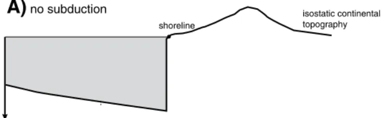
Figure 9. (A) Isostatic topography along a supercontinental margin. (B) Subduction is initiated along this margin. Associated dynamic subsidence leads to the flooding of the continental margin and to apparent sea-level rise. The additional volume of ocean created by dynamic subsidence leads to absolute sea-level drop. Compensation by water instead of air is not taken into account here, while it would further enhance subsidence of the flooded continental margin.

increase in the amount of flooded continents also implies that the oceanic surface is increased, which in turn contributes, though to a minor extent, to the decrease of the absolute sea level (Fig. 9). An end member of this paradoxical situation would be that the geological fingerprints of ESL rise accompany ESL fall.

Deciphering the eustatic signal from the geological record not only requires constraining the dynamic topography at the observation site, but also along all of the continent-ocean transitions. Some knowledge of the paleotopography of these margins is also required to allow for the evaluation of the amount of flooded surface that in turn participated in

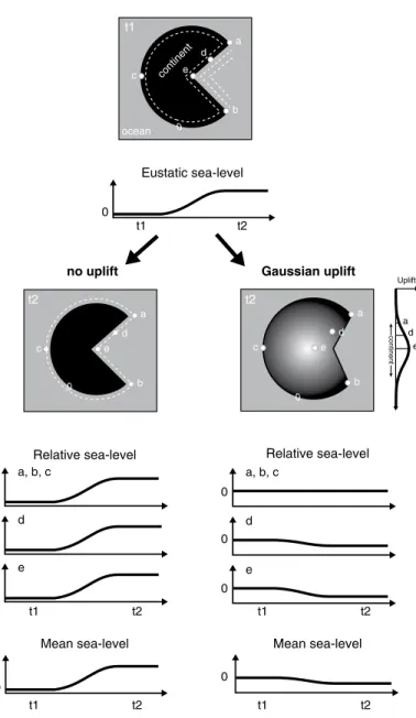
changing sea level. One could expect that averaging eurybatic variations from different places on Earth may allow the global signal to be extracted. The result would be unfortunately biased, since the vast majority of mea-surement sites are close to continental margins, which are more prone to dynamic subsidence or uplift. It implies that even averaging observations from different localities would not necessarily reflect the actual ESL varia-tions (Fig. 10). Dynamic tilt of supercontinent margins not only causes eurybatic changes, i.e., relative sea-level changes at the regional scale, but also absolute sea-level changes by modulating the bulk surface and volume of the oceans. Although we do not rule out the possibility that sea-level curves bear an ESL component in their signals, in particular, for the time scale of the aggregation and dispersal of a supercontinent, we neverthe-less emphasize that they should not be used as such. In order to properly assess second-order eustatic changes, only two solutions hold. Either vertical ground motion is comprehensively documented at the surface of Earth (and not only at continental margins), or the physical modeling capacities are improved to reach a prediction capacity that adjusts to the required resolution of eustatic charts. None of these solutions seems to be achievable in the near future.

CONCLUSIONS

We have shown that the apparent Middle Permian–Early Triassic low in ESL as well as the second-order variations reported on eustatic charts when Pangea was assembled cannot be strictly accounted for by the com-mon sea-level controlling processes. We suggest that the ESL rise expected from tectonics and glaciations during this period of time may have been hindered by the global effects of dynamic topography and endorheism, which both lower the absolute sea level. Furthermore, it follows that the ESL lowstand that is inferred from the geological record may not be an ESL low, but rather reflects an apparent sea-level drop produced by the deformation of solid Earth associated with thermal uplift and/or mantle plume dynamic uplift. Overall, the Permian–Triassic example highlights the difficulty in interpreting second-order (and beyond) sea-level changes, which should only be regarded as eurybatic, i.e., valid at the local scale. We anticipate that these disturbances may modulate the first-order curve

to an extent that does not challenge its common interpretations, but may explain the discrepancies between available charts.

ACKNOWLEDGMENTS

We thank the ANR GiSeLE (n°JCJC 601 01) for funding, and Arlo Weil, Michelle Kominz, and an anonymous reviewer for their comments that helped to improve the manuscript.

REFERENCES CITED

Allègre, C.J., Louvat, P., Gaillardet, J., Meynadier, L., Rad, S., and Capmas, F., 2010, The funda-mental role of island arc weathering in the oceanic Sr isotope budget: Earth and Planetary Science Letters, v. 292, no. 1, p. 51–56, doi: 10 .1016 /j .epsl .2010 .01 .019.

Alley, R.B., Clark, P.U., Huybrechts, P., and Joughin, I., 2005, Ice-sheet and sea-level changes: Science, v. 310, no. 5747, p. 456–460, doi: 10 .1126 /science .1114613.

Beard, J.A., Ivany, L.C., and Runnegar, B., 2015, Gradients in seasonality and sea-water oxygen isotopic composition along the Early Permian Gondwanan coast, SE Australia: Earth and Planetary Science Letters, v. 425, p. 219–231, doi: 10 .1016 /j .epsl .2015 .06 .004.

Blakey, R.C., 2008. Gondwana paleogeography from assembly to break-up—A 500 m.y. od-yssey, in Fielding, C.R., Franck, T.D., and Isbell, J.L., eds., Resolving the Late Paleozoic Ice Age in Time and Space: Geological Society of America Special Paper 441, p. 1–28. Bradley, D.C., 2011, Secular trends in the geologic record and the supercontinent cycle:

Earth-Science Reviews, v. 108, no. 1, p. 16–33, doi: 10 .1016 /j .earscirev .2011 .05 .003.

Braun, J., 2010, The many surface expressions of mantle dynamics: Nature Geoscience, v. 3, p. 825–833, doi: 10 .1038 /ngeo1020.

Brenchley, P.J., Carden, G.A., Hints, L., Kaljo, D., Marshall, J.D., Martma, T., Meidia, T., and Nol-vak, J., 2003, High-resolution stable isotope stratigraphy of Upper Ordovician sequences: Constraints on the timing of bioevents and environmental changes associated with mass extinction and glaciation: Geological Society of America Bulletin, v. 115, no. 1, p. 89–104, doi: 10 .1130 /0016 -7606 (2003)115 <0089: HRSISO>2 .0 .CO;2.

Burov, E., and Gerya, T., 2014, Asymmetric three-dimensional topography over mantle plumes: Nature, v. 513, p. 85–89, doi: 10 .1038 /nature13703.

t2 a d b c e t1 a e d

Relative sea-level Relative sea-level

Mean sea-level Mean sea-level

a, b, c d e 0 0 0 0 0 0 0 0 t1 t2 t1 t2 t1 t2 t1 t2 a, b, c d e Eustatic sea-level 0 t1 t2 Uplift continen t a d b c e a d b c e

no uplift Gaussian uplift

t2 0 0 0 ocean continen t

Figure 10. Schematic illustration of a fictive Earth undergoing eustatic sea-level rise between times t1 and t2. On the left diagram, no continental uplift occurs, and all the reference locations show the same relative sea-level variations. The averaged relative sea-level variations match the eustatic sea level. On the right diagram, Gaussian uplift affects the supercontinent with a maximum amplitude exceeding eustatic sea-level rise. Rates of uplift locally equal or exceed eustatic sea-level changes. Measurements of rela-tive sea-level variations vary between reference locations depending on their location with respect to the uplift signal. Averaging relative sea-level variations yields a mean sea-level drop while eustatic sea-level increases.