DOCUMENT OFFICE 36-412
RESEARCH LA ORiATORY OF ELECTRONICS MASSACHUSETTS INSTITUTE OF TECHNOLOGY
rT T TTrl" ( ' r (' T-TNT' . T.rr'' V
J.V-I I....RESEARCH LABORATORY OF ELECTRONICS V - .I.
RESEARCH LABORATORY OF ELECTRONICS
Technical Report 465 June 28, 1968
ANALYSIS OF DIGITAL AND ANALOG FORMANT SYNTHESIZERS
Bernard Gold and Lawrence R. Rabiner
(Manuscript received November 14, 1967)
Abstract
A digital formant is a resonant network based on the dynamics of second-order linear difference equations. A serial chain of digital formants can approximate the vocal tract during vowel production. The digital formant is defined and its properties
are discussed, using z-transform notation. The results of detailed frequency response computations of both digital and conventional 'analog' formant synthesizers are then presented. These results indicate that the digital system without higher pole correction is a closer approximation than the analog system with higher pole correc-tion. A set of measurements on the signal and noise properties of the digital system is described. Synthetic vowels generated for different signal-to-noise ratios help specify the required register lengths for the digital realization. A comparison between theory and experiment is presented.
---TABLE OF CONTENTS
I. Introduction 1
II. Digital Formants 2
III. Digital Formant Synthesizer 5
IV. Higher Pole Correction for the Analog System 20
V. Quantization Effects in Digital Formant Synthesizers 23
Acknowledgment 34
References 35
1. INTRODUCTION
The development of the theory of digital filters, 1, 2which has taken place in recent years, has made it feasible to simulate a wide variety of speech communication devices on a general-purpose computer. The formant-type speech synthesizer is one of the
3-5
devices that has been profitably simulated. In this report digital filter theory is used to study the behavior of a serial formant synthesizer for generating vowel-like sounds. This type of synthesizer, which incorporates analog components, has been used in the OVE series6 and in SPASS. 7 In the digital simulation of such devices, two new problems arise, sampling and quantizing. As is well known, a sampled-data filter is periodic in the frequency domain. Thus, a digital formant network obtained through simulation has a different frequency response from an analog formant network. As we shall see, the periodic frequency response of a digital formant network is actually a desirable feature, since it eliminates the need for the higher pole correction used with analog synthesizers. The quantization present in the finite-register-length computer
8
creates two disturbances: inaccuracies in the formant positions, and a wideband "noise" caused by round-off errors during the execution of the linear recursion. 9 10 These effects place a lower limit on the length of the registers, and therefore must be seriously considered in simulating digital filters on computers with small register lengths. Also, the component advances in digital hardware raise the possibility that a special-purpose all-digital speech synthesizer or formant vocoder could become a feasible device; clearly, knowledge of register length constraints becomes major design information.
A widely held misconception is that difficulties arising in computer simulation of speech systems can be avoided by increasing the sampling rate; however, quantization problems will generally increase in severity as the sampling rate is raised. Thus a sound theoretical understanding of the effects of both sampling and quantizing are necessary for the design of digital speech synthesis programs or special-purpose digital hardware synthesizers.
In Section II the digital formant network will be defined and discussed, and we shall show that although linear analysis, with z-transform techniques, is applicable, it is necessary, in practice, to consider carefully the lengths of registers to be used in computation. In Section III we shall study the frequency response characteristics of digital formant synthesizers theoretically and experimentally, utilizing only the linear model. Our primary purpose is to find the extent to which a digital synthesizer can approximate the vocal-tract transfer function. In Section IV we shall derive the characteristics of the higher pole correction network used in analog synthesizers. In Section V the quantization problem will be reintroduced and theoretical and experimen-tal methods will be applied to study the register-length problem.
II. DIGITAL FORMANTS
Using z-transform terminology, we can define the transfer function H(z) of a digital formant as
(1-2rcosbT+r2)z2
H(z)= 2
(1)
z - (2rcosbT)z + r 2
where T is the sampling interval, and r and b are defined by reference to the z-plane pole-zero diagram of Fig. 1. The frequency response of the digital formant is obtained by setting z = ej t in Eq. 1. Except for the frequency-dependent scale factor in the numera-tor, this frequency response can be obtained geometrically from Fig. 1 by measuring
the distance from any point on the unit circle (at an angle coT) to the poles, the magnitude of H(e jwT ) being inversely proportional to the product of the distances from that point to the poles, and directly pro-portional to the product of the dis-tances to the zeros, which in our case are unity. The significance of r is illuminated by letting r =
-aT
e , so that the parameter a may be interpreted as a
half-bandwidth radian frequency. It
can be seen from Eq. 1 that H(1) 1, which shows that the digital formant has the correct DC gain indenendent of the resonant
fre-Fig. 1. Z-plane pole-zero diagram for quency; this is accomplished by
Fig. 1. Z-plane pole-zero diagram for
digital formant. making the numerator dependent
on the pole positions so as to always satisfy this condition on the DC gain.
The transfer function H(z) can be realized approximately in a variety of ways; approximately because no indication of the quantization problem appears in Eq. 1. Thus, the recursive relation,
y(nT) = 2r cos (bT) y(nT-T) - r2y(nT-2T) + (1-2rcosbT+r 2) x(nT) (2) permits the variables x(nT) and y(nT) to take on any real values, whereas in the computer these variables are always contained in finite-length registers. A convenient way of
representing the computation of Eq. 2 is by the "network" of Fig. 2. The triangular boxes represent unit delays of time T, the rectangular boxes are the fixed multipliers,
y (nT-2T)
y (nT)
Fig. 2. Digital network representation #1 of a single formant.
that is, the coefficients of the recursive equation (2), and the sum is represented by the circle with the plus sign. These elements are the basic ones for any general system of linear recursions. Computationally, Fig. 2, as well as Eq. 1, is interpreted as follows: a new sample x(nT) appears at the input. This signal is multiplied by the fixed number
(l+r2-Zr cos bT); the multiplications indicated by the other two rectangular boxes are carried out, all indicated products are summed, and the appropriate register transfers are performed, to fulfill Eq. 2. The system is now ready for a new input sample.
Because of the linearity of the network of Eq. 1, it is possible to exchange the sequence of operations. For example, Fig. 3 represents a different sequence of com-putations leading to the same transfer function H(z) in Eq. 1. Although the difference
Fig. 3. Digital network representation #2 of a single formant.
between the networks of Figs. 2 and 3 may seem trivial, if one remembers that the actual computations involve finite register lengths, these differences may be significant. To illustrate, assume that 1 + r 2 - 2r cos bT = . 01 for a given system. If an input sample x(nT) of magnitude 20 appeared, the product is less than unity and would be truncated to zero. Thus, the system of Fig. 2 exhibits a noticeable nonlinear effect if the input
signal level is too small. The same signal applied through the network of Fig. 3, how-ever, might not exhibit such an effect because the first portion of the network (up to the
3 X
final multiplier) could have boosted the signal level to well above 100. Thus, although the "linear" behavior of the networks of Figs. 2 and 3 is identical, the actual behavior of the two could be markedly different.
20 m 0 z -j _ -20 -J a-u -40 -60 -1U U - -a U- -r -
-U 1VUUU LUUU OUUU 4UUU 3:UU
FREQUENCY IN Hz
Fig. 4. Frequency response of a digital formant.
In the remainder of this section and until Section V, the finite-register-length prob-lem will be ignored and the frequency response characteristic of the digital formant net-work will be studied, with Eq. 1 and Fig. 1 used as the starting point. H(z) actually has an infinity of poles, occurring at the frequencies (b/2rr ± nfr)Hz with n = 0, 1, 2,... and fr = 1/T. Thus, the frequency response of the digital formant is periodic, with a
r T
made explicit for the digital formant by writing IH(eJoT) I, that is, the magnitude of H(z) at any angle wT on the unit circle,
2
jH(ejWT) 1 - 2r cos bT + r (3)
2j =2 /) 2 1/2 (3)
[l+r -2r cos (-b)T] [l+r -2rcos (+b)T]
JH(ejoT) is clearly periodic in the angle wT with period Zrr, and this is equivalent to periodicity in frequency with period fr Also, the resonance effect is clearly seen by means of the left side of the denominator, which becomes small when (-b)T = nr, n = 0, ±1, ±2, ... , thereby yielding the type of result sketched in Fig. 4.
4
CENTER FREQUENCY- 500 HZ BANDWIDTH- 60 HZ
III. DIGITAL FORMANT SYNTHESIZER
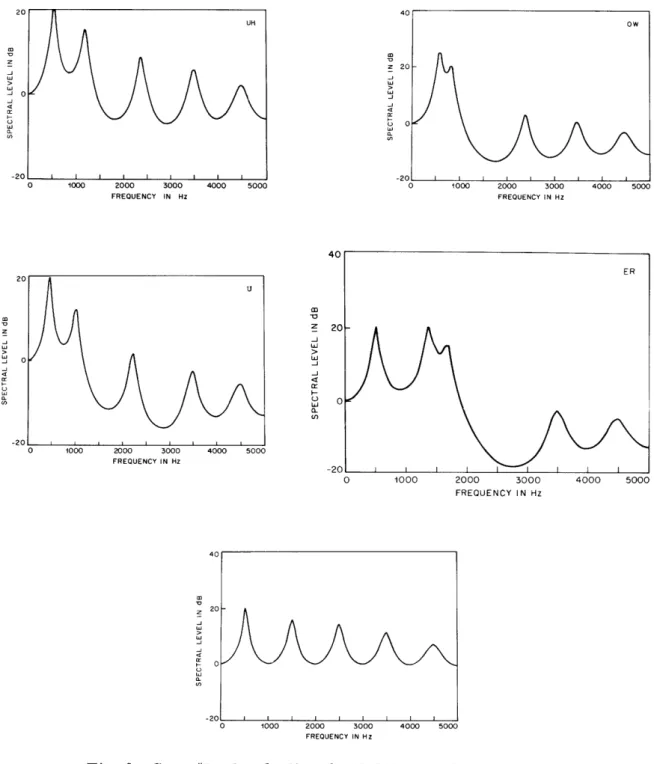
It is, of course, the repetitive nature of the frequency response of the digital mant network which suggests that it resembles more closely (than does the analog for-mant network) the repetitive frequency response of the vocal tract. The upper curve of Fig. 5 indicates the frequency response of an acoustic tube excited at one end and open at the other. (We have assumed equal bandwidths for all resonances.) This simple model is a representation of an ideal neutral vowel. If the sampling time T is chosen to be 0. 5 msec, then a digital formant at 500 Hz has repetitive modes at the same fre-quencies as the tube, while a single analog formant at 500 Hz does not at all resemble the tube. The rest of the curves in Fig. 5 show a comparison among 5 formant, analog, and digital (T = 10 sec) approximations to the tube. It is clear that, for this case, the digital system is a good approximation to the tube, whereas the analog system needs a correction network to compensate for the high-frequency fall-off characteristics of cas-caded analog formants.
--(
0 1 2 3 4 5
FREQUENCY
(kHz)-Fig. 5. Digital and analog approximations to the transfer function of an acoustic tube, open at one end and closed at the other.
A mathematical representation of the distributed parameter vocal-tract system is quite difficult, and we are not able (nor have we really tried) to create a purely theoret-ical argument for choosing either the digital or analog formant as the better approxima-tion to the actual vocal tract. It can be argued, however, that an analog formant synthesizer consisting of a large number of resonators and higher pole correction can serve as a criterion for the correct frequency response characteristic of the vocal tract. The standard that we have adopted uses 10 cascade resonators and an improved higher pole correction. (The nature of this improvement will be examined in Section IV.) We denote this standard configuration #1. In the rest of this section we shall present and discuss experimental comparisons between system #1 and the three following systems.
#2 10-pole digital formant synthesizer with 20-kHz sampling. #3 5-pole digital formant synthesizer with 10-kHz sampling.
#4 5-pole analog formant synthesizer with improved higher pole correction. As we have indicated, we have guessed that a digital synthesizer does not need any higher pole correction, and no such network is used in systems #2 and #3.
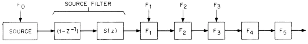
Figure 6 represents system #3. The resonance frequencies F1, F2, and F3 are
variable and correspond to the three lowest resonances in the voiced-speech spectrum,
FO SOURCE FILTER F, F2 F3
SOURCE (1 - Z ) S( Z)
~
F1 F2 P F3 F4 F5Fig. 6. 5-pole, 10-kHz digital formant synthesizer.
and thus determine, for example, the particular vowel sound that is generated. The fixed resonators F5 and F4, with resonances at 4500 and 3500 Hz, help provide the
cor-rect over-all spectrum shape. S(z) represents a formantlike digital network, which has -1
been recommended as a suitable source filter, and the transfer function 1 - z approx-imates the mouth-to-transducer radiation. Each of the digital formant networks is of the form given in Figs. 2 or 3 and has a transfer function of the form of Eq. 1. Thus the transfer function of the entire synthesizer is given by
5
F(z) = S(z)(l-z-l) Fi(z),
i=l
with (4)
(l+r 2-Z r i cos biT) zZ
Fi(z) = z -2 (Zri cosbiT)z + r2
i
For the 10-pole digital, 20-kHz system #2, five additional digital formants at 5500, 6500, 7500, 8500 and 9500 Hz have been inserted into the chain of Fig. 6.
Each digital formant is specified by values of the parameters ri and bi . To change
-2rgiT
these parameters into frequencies, we use the relations r. = e 1 and b = ZTrfi, so that fi is the resonance frequency, and gi is the half-bandwidth expressed as a Herzian
1 1 11
frequency. Table 1 shows the values of fl, f2' and f3 chosen for each of the 10 vowel
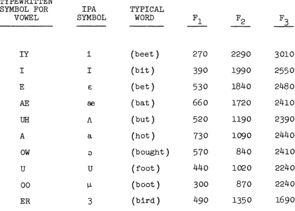
sounds analyzed by us. Table 2 shows the bandwidths of all of the formants; the same fixed values were used throughout for both digital and analog cases. The values and extrapolations for higher formants are based on data by Dunn. 12
Table 1. Formant frequencies for the vowels. TYPEWRITTEN SYMBOL FOR VOWEL IY I E AE UH A OW U 00 ER
Table 2. Analog and digital resonator bandwidths and center frequencies,
RESONATOR Fl F2 F3 F4 F5 F6 F7
F8
F9 F1O Variable Variable Variable 3500 4500 5500 6500 7500 8500 9500Q
Variable Variable Variable 2016
129
64
2 IPA SYMBOL i I 6 ae A a U3
TYPICAL WORD (beet) (bit) (bet) (bat) (but) (hot) (bought) (foot) (boot) (bird) F1 270 390 530 660 520 730 570440
300 490 F2 2290 1990 1840 1720 1190 1090 840 1020 870 1350 F3 3010 2550 2480 2410 2390 2440 2410 2240 2240 1690 CF (Hz) BW (Hz) 60 100 120 175 281458
722 1250 2125 4750 7sI m z in 20 -J w w -J -J 4a i- 0 O (-) 2 wen, 0 1000 2000 3000 4000 5000 FREQUENCY IN H FREQUENCY IN Hz FREQUENCY IN Hz FREQUENCY IN HZ cn Z > w w J t o w
a
-i 0 1000 2000 3000 4U00 nUUu 0 1000 2000 3000 FREQUENCY IN HZ FREQUENCY IN HZFig. 7. Case #1. Amplitude frequency response -10-pole analog. 4000 ,5000 8 z w L'J -J -w 0. cn 2 4 -LL -) C-j cr (C) a-vn 40 -2 Z > O -20 -j w w -: 0 0 w (I) -20 rn 1 1n 7~l
~
TAnA n\ -_ - - - , ,40 UH 20 0 1000 2000 3000 FREQUENCY IN HZ 4000 5000 m I z LUI w U a w (_)W r, 40 Z 20 w t 0 --20 0 1000 2000 3000 FREQUENCY IN HZ FREQUENCY IN HZ 40 20 0 -20 FREQUENCY IN Hz FREQUENCY IN Hz
Fig. 7. Case #1. 10-pole analog (concluded).
9 m -i z H C) LU 0i mUL' EL U) I I I I I I I I I 4000 5000 co z w J a: H c) 0u U) z -w -j -J 0: n U a. U)
_
I
__
_ __I ----
1_1__11_1__·_11_11^I_-_-^-
___
40 z -J LU w -j 0 LU a Un 20 -20 FREQUENCY IN HZ 20 z 'D Z -J LU > Ld-J -a (-0 -20 FREQUENCY IN Hz FREQUENCY IN HZ a z -J > LU a-O3 0 1000 2000 3000 4000 5000 FREQUENCY IN HZ 0 1000 2000 3000 FREQUENCY IN HZ 4000 5000 O 1000 2000 3000 4000 5000 FREQUENCY IN Hz
Fig. 8. Case #2. Amplitude frequency response - 10-pole digital, 20-kHz sampling frequency.
10 40 20 z .u J bI Z O3 cr L -20
0 1000 2000 3000 FREQUENCY IN HZ 4000 5000 FREQUENCY IN HZ z -j Li -J -j I-'i 0L M 0 1000 2000 3000 4000 5000 FREQUENCY IN Hz z -J w w -j 4 w a-en 40 20 0 -20 FREQUENCY IN Hz 0 1000 2000 3000 4000 5000 FREQUENCY IN HZ
Fig. 8. Case #2. 10-pole digital, 20-kHz (concluded). sampling frequency 11 UH 40 20 z Z I wJ w I. -x Cr I v, -20 20 , z -J w w -J -J M L-an tO 0 -20 I I I I I I I I $ - - I- ----~'1- -"' 1' "^`11~~111--·111_-·mllI ___- _-_ _....-. .
FREQUENCY IN HZ
FREQUENCY IN HZ
0 1000 2000 3000 4000 5000 FREQUENCY IN HZ
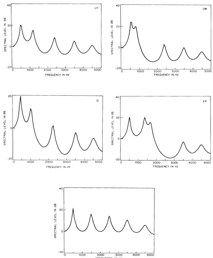
Fig. 9. Case #3. Amplitude frequency response - 5-pole digital, 10-kHz sampling frequency.
12 .U I 4o z 20 J .d I , "I FREQUENCY IN HZ E FREQUENCY IN HZ - cv-- I I I I I I I I I I I .4 I I1 II .. FREQUENCY IN HZ E I -1 I .1 I I
0 1000 2000 3000 FREQUENCY IN Hz 4000 5000 FREQUENCY IN HZ m z Z UJ 4 -I M U a. U) 0 1000 2000 3000 4000 5000 FREQUENCYIN HZ m z 20 I -I > .J O L -2 0 1000 2000 3000 FREQUENCY IN HZ 0 1000 2000 3000 4000 5000 FREQUENCY IN Hz 4000 5000
Fig. 9. Case #3. 5-pole digital, 10-kHz sampling frequency (concluded). 13 II J 0 -20 UH I I I I I I I I I In l _ _
I_
_111____
^^
-o u ii Z' II -4 I I "I m -oI I z ,,> I ----Go z U) w U] -J a. U1) U) 0 1000 2000 FREQUENCY IN Hz FREQUEI 3000 4000 5000 ICY IN HZ 0 1000 2000 3000 4000 5000 m r, z Z -j w _j a: U a I-U) a-U) FREQUENCY IN H FREQUE ) z -J > -a w w a: U a U, (L IA) FREQUENCY IN H FREQUEI
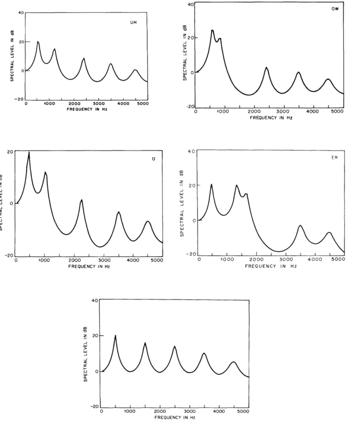
Fig. 10. Case #4. Amplitude frequency response -5-pole analog. 14 z -J w n LI z -j w w -J -J 0 U)
I
w a (n z _J g QuA U) :NCY IN Hz NCY IN Hz _ _m z Z -j Lu tu -J -j 0 LuJ a CL U) FREQUENCY IN Hz 20 m V z J -j -r a Luw a-(2, -20 0 1000 2000 3000 FREQUENCY IN Hz 40 m en z -j Lu LuJ -J > w J L a-en to 20 -20 FREQUENCY IN HZ 4000 5000 FREQUENCY IN Hz FREQUENCY IN Hz
Fig. 10. Case #4. 5-pole analog (concluded).
15
-- l---- I
1---·111-·---The analog formant synthesizers are the classical vowel synthesizer treated by Gunnar Fant. 3 They consist of 5 (for case #4) or ten (for case #1) analog resonators of the form
*
H(s) = (5)
(s-s 1) (ss 1)
an additional analog resonator of 200-Hz center frequency and Z50 Hz bandwidth for the source filter, a differentiator, and a higher pole correction (which will be described in greater detail in Section IV).
Given the 10 vowels listed in Table 1, a total of 40 frequency response curves had to be experimentally determined in order to compare systems #1, #2, #3 and #4. The measurements for systems #2 and #3 were made by passing a unit sine wave through a simulation of the system and determining the peak output amplitude after the transient response of the system had subsided. The frequency of the input was varied from 50 Hz to 5000 Hz in 50-Hz steps. The data for systems #1 and #4 were theoretically calcu-lated from the synthesizer system functions. Figures 7 through 10 show results for the four systems for each of three vowels. In these figures, the logarithmic magnitude (in dB) is plotted on a linear frequency scale. The contribution of the source filters is omitted from these curves and will be treated separately. No generality is lost thereby, since, as we shall see, it is a simple matter to combine the effects of the source and resonators.
Figures 11, 12 and 13 show plots of the differences between spectral magnitudes of systems #2, #3, and #4 relative to the reference system #1 for each of the vowels IY, A, and OO0. (Table 1 shows the IPA symbols and our typewritten equivalents for the vowels.) We see that the 10-pole, 20-kHz digital system #2 is extremely close to the reference system. This strongly indicates that higher poles of the vocal-tract transfer function are automatically, and more or less correctly, taken into account by the repetitive nature of the digital formant frequency response. We also note that this intrinsic correction is actually more accurate than the quite good analog higher pole correction used in our computations. These results are generally valid for all of the vowels.
Comparison of system #3 with the standard is of particular interest, since a 5-pole, 10-kHz system appears to be a good compromise design for a possible hardware version of a digital formant synthesizer. The peak difference between the magnitude curves for systems #1 and #3 is listed in Table 3, for each vowel. On the basis of this result, it seems reasonable to expect that a 5-pole, 10-kHz digital vowel synthesizer should produce synthetic vowels of quality comparable to a well-designed 5-pole analog vowel synthesizer that includes a higher pole correc-tion. Informal listening re-enforces this expectation.
+6 +4 2 SYSTEM -2 -4 - SYSTEM 4 0 1 2 3 4 5 FREQUENCY
(kHz)--Fig. 11. Spectrum magnitude differences for IY.
I -o + + + 0 1 2 3 4 5 FREQUENCY (k Hz)
--Fig. 12. Spectrum magnitude differences for A.
m 'a 6 4 2 0 -2 -4 -6 0 1 2 3 4 5 FREQUENCY (kHZ) -_
Fig. 13. Spectrum magnitude differences for 00.
17 -6 4 -2 SYSTEM #3 -2 - SYSTEM #2 SYSTEM #4 -4 --6 SYSTEM # 3 SYSTEM #2 SYSTEM #4 I L_ , - _ - _ - -- --- - -- I
increases the deviations of systems #2, #3, and #4 from the reference. Figure 14 shows the frequency responses of the two digital and one analog source filters. (We have included the differentiator as part of the source filter.) The plots are
normal-ized so the peaks are set to 0 dB for all three cases. With the inclusion of source
Table 3. Peak difference between systems #4 and #1 for the vowels.
VOWEL IY I E AE UH A OW U 00 ER AVERAGE m Li D Z z 0
PEAK DIFFERENCE BETWEEN SYSTEMS #4 AND #1
3.69
2.42 db 2.18 2.00 1.56 1.62 1.44 1.25 1.16 0.65 1.80 db 0 1 2 3 FREQUENCY (Hz)-_Fig. 14. Source filter characteristics.
filters the frequency response of system #2 is within 1 dB of the reference for all vowels and all frequencies. The peak difference, in the worst case, (for IY) between system #3 and the reference is 7.48 dB at 5 kHz. For all vowels except IY and for all frequencies below 4 kHz, the difference never exceeds 3.5 dB. It is possible that a digital source filter with slightly decreased bandwidth could bring the two results closer together.
19
IV. HIGHER POLE CORRECTION FOR THE ANALOG SYSTEM
The material to be presented here is incidental to the main line of development of this report and deals only with the question of the higher pole correction for analog for-mant synthesizers. The higher pole correction is used to approximate the higher modes of the vocal tract which are not explicitly present in the synthesizer. The frequency-response magnitude of this network (to be referred to as Q(w)) was derived by Gunnar Fant, 14 and is 2 Rk
IQk(o)
|
el
with (6) k k 8 1 n=l (2n-1) 2in which it has been assumed that k analog formant networks are used to approximate the vocal tract, and o1 is the radian frequency of the first formant. In order to make Qk(w) into a network with fixed rather than variable parameters, col is usually chosen to be an average, say, 2 X 500 rps.
Our observations have been that the 5- and 10-pole analog synthesizers, both utilizing the Qk( ) specified by Eq. 6, nevertheless yielded substantially differing
frequency-response curves. In fact, results were obtained which appeared to be qualitatively wrong. The result was that the 5-pole system was attenuated more with increasing fre-quency than the 10-pole system. Given that the 10-pole system utilized rather wide band-widths for formants 6, 7, 8, 9, and 10 and that the higher pole correction presumably corrects for higher modes having narrower bandwidths, we should presume that the reverse result would have been observed. We conjectured that the approximations leading to Eq. 6 were too gross and, accordingly, we present a somewhat more refined formula for approximating the higher modes of the vocal tract for an analog formant synthesizer.
We begin with the assumptions used by Gunnar Fant in his original derivation: The vocal tract filter during vowels can be represented in the frequency domain by the infi-nite product * 00 s s P(jw) = n n (S n) ( ns*) 20
2 2 k C oo H n n n n=1 2 1/2 n=k+1 2 1/2 [2-o2) + (2oZ^)2] [(2n2 ) +(20n )Z] Pk(J O) Qk(jo), (7)
where on and won are the damping term and resonant frequency expressed in radians per second, and Pk(jw) represents those k formants that are explicitly constructed in the synthesizer. Thus Qk(jo) appears as the product from k+l to infinity of those formants that are not built into the synthesizer. To approximate Qk(jw) |, Gunnar Fant first
assumes that an is small enough to be set to zero for all n. This yields
00oo 11
IQk(jw)
I
= 11 2 ' (8)n=k+l 1 W
on
and taking the logarithm of both sides, we obtain
0
In Qk(jo) - in - 1 (9)
n=k+1 On
Gunnar Fant then expands the logarithm as a power in (1/2n) series and uses only the first two terms, which leads to Eq. 6. Our extension includes an extra term in this series, so that
00 4 00
in 2 2Qk(J°) + E 14 (10)
n=k+l1 °n n=k+l 'on
If we now take the modes to be that of a straight pipe of length , the values of n are periodic and are wn = (2n-l)w1 = (2n-1) 2, where c is the velocity of sound.
2 oo 4 oo
wrr 1 wrr 1
Making use of the identities 2 and 4 we arrive at
n=l (2n-1) n=1 (2n-1)
with (11)
k
k 4 n= 1= (2n1)4'
21
The first term in Eq. 11 is the usual higher pole correction. Figure 15 shows plots of the first term of Eq. 11 (or Eq. 6) for the two cases k = 5 and k = 10. It is evident that both 5- and 10-pole systems need this standard higher pole correction.
50 40 30 20 0 1 2 3 FREQUENCY (kHZ) -5 m V
Fig. 15. First-order higher pole cor-rection.
0 1 2 3
FREQUENCY
(kHz)--4 5
Fig. 16. Second-order improvement in higher pole correction.
Figure 16 shows plots of the second term in Eq. 11, namely, the expression exp
( )
Lk. We see that if a 10-pole synthesizer is used, this extra refinement is insignificant but if 5 poles are used, a reasonably significant correction is added. It should be noted that at frequencies above approximately 4 kHz the cross modes of the vocal tract are of significance. Thus the significance of this additional correction factor is diminished. m ' 10 0 8 6 5 RESONANCES 4 2 10 RESONANCES O l l l IV. QUANTIZATION EFFECTS IN DIGITAL FORMANT SYNTHESIZERS
The finite length of the registers containing the signals flowing through the networks of Figs. 2 and 3 influences the results in several ways. First, the coefficients of the difference equation (2) cannot, in general, be specified exactly, so that the true pole positions may be in error. This is a fixed error and easily computed by comparing the quantized and nonquantized coefficient values. Second, the signals are perturbed by quantization during each iteration of the computation. If signal-level changes from one iteration to the next are large relative to an individual quantum step, then it seems rea-sonable to hypothesize 15, 2,9, 10 that signal quantization behaves as additive noise, all such sources of noise are uncorrelated, and each sample of this noise is uncorrelated with past and future samples. Such a hypothesis greatly simplifies the formulation of the digital network quantization problem and makes it easier to interpret experimental results, but clearly there must first be some indication that valid predictions can be made on the basis of such a simple hypothesis. Therefore we shall first study the valid-ity of the simple additive noise, and then discuss some of the results that have been obtained, these results being illuminated by reference to the model.
Fig. 17. Noise model formant network.
Figure 17 is a modified version of Fig. 3, wherein three noises el, e2, and e3 are
added, corresponding to the round-off or truncation errors implicit in each of the three multiplications. We assume that each noise sample produced at every recursion is uncor-related with all other noise samples produced by the same noise generator during other recursions, and that e1(nT), e2(nT), and e3(nT) are mutually uncorrelated even for
the same iteration. Such an assumption is surely wrong if, for example, any two coef-ficients in the recursive equation were exactly equal, so that our hypothesis will not include such special cases. Thus all that needs to. be known statistically are the
one-dimensional probability distributions associated with each of the three random vari-ables. Again, a reasonable assumption is that el, e2, and e3 are uniformly distri-buted over a quantization interval and for fixed-point arithmetic, independent of signal
level. We also specify that quantization levels be uniformly spaced (linear quantization of the signals). Whether or not the probability distributions depend on the sign of the signal is determined by the precise manner in which quantization is effected. Let us examine this point more closely.
In a digital computation, the product of two numbers can occupy a register of twice the length of each of the numbers. For example, the product of the two 5-bit positive binary numbers 0. 1011 and 0. 1110 yields the 10-bit product 00. 100 111010. To store the result in a 5-bit register requires that the five lower bits be removed, and this may be accomplished via truncation, wherein the low-level bits (after a 1-bit left shift to restore the original decimal point placement) are simply removed, thereby yielding
0. 1001. Alternatively, the result may be rounded-off to the nearest quantization level, to yield, in this example, the product 0. 1010. Now, this last operation results in the
uniform probability density shown in Fig. 18a, while Fig. 18b holds for trun-cation of a positive signal, and Fig. 18c holds for truncation of a negative signal. Thus, truncation introduces a quasi-periodic component of the resultant noise. If a sign-dependent truncation were
per--Eo Eo ±~~~~JI
~-
a iL_ L& -VI±JX1i _LJ-1± 1 -d. IA) 41L- J-- -14L UIP-Eo Eo a LUl-lIL VI11 GUUtU LI-U LU L;1U OU.lL A
2 2 either Fig. 18b or 18c regardless of
sig-Px (a) nal sign, then only a DC component would
(b) be induced in the noise spectrum. The
importance of raising these seemingly Eo
trivial points lies in the fact that different hardware configurations or different
com-0 ) EQo a puter programs would be required,
deter-mined by how the extra bits were chopped
P x (a) off, and the programmer or designer ought
(c) to be cognizant of the effects of these dif-ferent realizations on the resultant noise.
Eo
Returning now to the noise model of Fig. 17, let us consider the noise
gen--E° 0 a erated at the output of the digital filter
Fig. 18. Probability density functions caused, say, by el(nT). The variance
of noise. of this noise at any time nT created by
a noise sample at m = 0 is given by 2h h2(nT), where (r2 is the variance of e(nT), and h(nT) is the network unit pulse1
response. Similarly, the variance created by a noise sample at m = 1 is o-2h2(nT-T). Proceeding in this way, one can construct the formula for the output variance resulting from e1(nT) to be
n
nT 2(mT). (12)
~dl
m=O
This formulation has been explained in greater detail elsewhere.2' 10
The variance -2 of e1(nT) can be obtained by inspection of Fig. 18, and is Eo/12,
where Eo is the magnitude of a single quantization step. To obtain the total variance caused by all of the noise sources indicated in Fig. 17, we need only add the contribu-tions arising from each noise source; this yields
2 2 2 2 2/6 E h=
d a'Jdl + d2Z + = 6m0 (13)
To obtain the total variance caused by all noise sources in a more complex network such as the 3 cascaded digital formant networks shown in Fig. 19, we add again the variances
Fig. 19. Noise sources in a cascade of 3 formants.
resulting from each source, using that unit pulse response that describes the passage of that particular source through the system. For example, e(nT) (Fig. 19) passes through all three digital networks, whereas e7(nT) passes through only the final one;
thus, the h(nT) used to compute 2dl is different from the h(nT) used to compute crd7 In a digital system wherein all poles are within the unit circle, the summation (12) converges to a finite value, so that, if we let the upper limit n of (12) become infinite, we have an expression for the "steady-state" variance of the system. Physically, one would expect this "steady state" to be reached in a time that is approximately the same
as the transient response time of the system. For this case, evaluation of (6) for specific networks is algebraically less cumbersome and, indeed, crude approximations can be made which increase physical insight into the noise effects and perhaps may help suggest improvements in configurations. Before further elaboration of these statements, let us first describe an experimental method of measuring the noise in an arbitrary sys-tem, and then show some results comparing theory with experiment which tend to verify
our noise model.
The digital transfer function V(z) in Fig. 20 represents the complete 5-pole, 10-kHz formant synthesizer which we have described, including source and radiation transfer
noise
Fig. 20. Noise measurement on the digital formant synthesizer.
functions. A is an attenuator such that the output is a small fraction of the input, and x(nT) is a periodic train of pulses of 1 sampling interval duration. Since the amount of
quantization noise is not a function of the input signal level, points b and c in Fig. 20 contain approximately equal noise levels. Attenuating the signal from b to d should not change the signal-to-noise ratio at these points; therefore, the noise at point c is appreciably larger than the noise at point d, although the signal levels are equal. Thus,
subtracting the two signals should give a reasonable measure of the noise, especially if significant noise is present.
In order to compare theory and experiment, the noise variance from V(z) should be measured by using the arrangement in Fig. 20, and this result should be compared with that obtained by application of Eq. 12 to the same system. We did this for the 10 vowels listed in Table 1. The variance was measured by averaging the sum of the squares of 3500 samples of the noise. Measurements showed that the noise had zero mean. The precise cascading of the components of V(z) is shown in Fig. 6. The wrong value of the damping term for the source filter was inadvertantly used in this experiment (60 Hz instead of 250 Hz), but this should have no effect on the general validity of this compar-ison between theory and fact. Comparisons of the variances, expressed as octal num-bers, are shown in Table 4. Although the agreement is not perfect, it is clearly close
enough to encourage use of our simple noise model.
We now can return to the problem of crudely approximating the noise generated by a single digital formant. With the use of the result1 0
o00
h2(nT) = - H(z) H(1/z) z- dz, n=O
(14)
where H(z) and h(nT) is a transform pair and the integral is around the unit circle, com-putation of Eq. 12 is easily performed by using the calculus of residues if H(z) is a
Table 4. Comparison of theory and experiment for predicting noise.
MEASURED NOISE 702,664 125,574 101,110 57,674 51,414 51,050 50,700 53,460
41,044
27,574 THEORETICALLY DETERMINED VALUE735,547
114,717 104,036 52,241 52,24155,346
52,763 52,242 42,123 27,465digital formant network. The approximate result obtained when the poles are close to the unit circle is E/12E, where E = 1 - r. Since the gain at resonance of a digital
for-0
mant network is also inversely proportional to E, it follows that a network will amplify the noise proportionally to its resonance gain. From this it follows that the noise gen-erated by the digital formant network can be altered by rearrangement of the order of the chain. For example, since F5 has a higher resonance gain than F1, it should appear
earlier in the chain because thereby all of the noise generated by the system following F5 does not pass through F5 and is not amplified as much.
We see that when using a simple noise model quantization considerations help us decide how the synthesizer is to be arranged, and in what order the formant networks should be arranged to keep the noise low. Other considerations also enter into such decisions. For example, it has been conjectured that the system is less sensitive to transient disturbances following formant frequency changes if the higher formant net-works precede the lower ones. Intuitively, this argument resembles the noise argu-ment and leads to the same or similar arrangeargu-ment. Another consideration is dynamic
27 VOWEL IY I E AE UH A OW U 00 ER
range; the problems arising here are equivalent to those arising in analog systems wherein the formants are arranged so that the signal becomes neither too large nor too small. The comparisons in Figs. 2 and 3 allude to this problem.
A further benefit may be derived by closer examination of the precise way in which the computation for a single digital formant is carried out. Often, the way the
compu-tation is performed depends on the computer; in the sequel we shall illustrate by an
Fig. 21. One way of realizing a digital formant on TX-2 computer.
example, using a TX-2 computer program. The TX-2 is a fixed-point computer with an automatic left shift after multiplication so that if the decimal points directly follow the high-level bit (as in the example already given), then the product will automatically have the same decimal point position. This makes it convenient to treat all numbers as decimal fractions. The coefficient Zr cos (bT) in Eq. 2 is usually greater than unity, however, and the program must take this into account. Two ways of doing this are illustrated in Figs. 21 and 22. Multiplications by powers of two are only shifts, of course, so that the restriction of treating numbers as decimal fractions does not apply. We intuitively feel that the configuration of Fig. 21 leads to better signal-to-noise ratio, since the round-off or truncation caused by the multiplications in either case is the same but the signal levels in Fig. 21 are maintained higher. Experimental results indicate that the noise variance of the formant network by using Fig. 21 is approximately double that obtained by using Fig. 22.
Finally, we present experimental results that make it possible to specify the required register lengths needed for each of the data-carrying registers in each of the networks. This is accomplished in the following way: A given vowel is generated by setting formants 1, 2, and 3 to one of the rows of values in Table 1; the digital synthe-sizer is excited by a periodic pulse train corresponding to the pitch (for most experi-ments the pitch was set to 125 Hz), and the magnitude of this excitation is systematically
X (nT)
Fig. 22. Alternative method of realizing a digital formant on TX-2 computer. reduced until the effects of quantization are audible. Also, the signal-to-noise ratio (defined as the ratio of the rms of the output signal to the rms value of the noise) is measured. During the execution of the program, peak magnitudes are recorded for each register in the system. From this information, it is possible to construct a table for any given configuration listing the number of bits needed for each register. Referring to Figs. 2 and 3, we see that only two registers per digital formant need be listed, for example, in Fig. 2, the input and output of the numerator multiplier. The registers containing y(nT-T) and y(nT-2T) will be of the same length as the register containing y(nT).
For convenience, we express each digital formant H(z) as the ratio N(z)/D(z). The chain drawn in Fig. 23 shows the sequence of operations in one particular run. Note that we have omitted the numerator factors NS, N4, and N0. These are fixed multipliers,
and should not be included, since they introduce extraneous and unnecessary noise.
Table 5 shows the required register length associated with each member of the chain. The particular ordering of the chain was chosen to try to pass as little noise as possible through the high-gain formants; hence, F5 and F4 were put at the beginning. The
signal-to-noise ratio, defined as the rms signal divided by the rms noise, is listed in the last column of Table 5, in bits. Thus, for example, 8 bits corresponds to a ratio of
--msC
I L
SIGNAL TO NOISE RATIO
MEASURED HERE
D IrN D N , OUTPUT
®1
22 2 s
c o
Fig. 23. The 540321 sequence of digital formants.
Table 5. Register lengths for 540321 synthesizer configuration. NODE # VOWEL 1 2 3 4 5 6 7 8 9 10 S/N IY 10 12 13 11 12 14 13 14 13 8 4.5 I 10 12 13 11 12 13 12 12 12 8 4 E 10 12 13 11 12 12 12 12 12 9 4.5 AE 10 12 13 11 11 12 11 11 11 9 4 UH 10 12 13 11 11 12 11 10 11 8 5 A 10 12 13 11 11 12 11 10 11 9 4.5 OW 10 12 13 11 11 12 11 9 12 9 4 U 10 12 13 11 11 12 11 10 11 7 4 00 10 12 13 11 11 12 11 9 12 7 4 ER 10 12 13 11 11 11 11 10 12 8 4 Maximum over 10 12 13 11 12 14 13 14 13 9 all vowels
256, while 8 -bits is /512. Listeners agreed that this configuration corresponded most
closely to the threshold of audible noise. Speaking rather loosely, if we allow a rea-sonable tolerance for problems such as transients caused by formant changes, it would seem that a computer with an 18-bit register length would satisfy fidelity requirements on a digital formant synthesizer.
We should keep in mind that the numbers obtained hold for a 5-pole, 10-kHz system. If the number of poles is increased, the situation worsens. More noise is generated and the problem of maintaining fairly uniform dynamic range becomes more difficult. If the sampling rate is increased, the situation also worsens, since the poles come closer to the unit circle, so that the gain of the system increases. Again, this means that it becomes more difficult to uniformly distribute register lengths, although the effect on the signal-to-noise ratio is not clear.
In contrast to the configuration of Fig. 23, where gains were judiciously adjusted, Fig. 24 and Table 6 show the result of a rather arbitrary arrangement of formants. Notice that although the register lengths need to be larger in this case, comparable signal-to-noise ratio results. Thus, we see that some care in the ordering of the ele-ments results in a more efficient system, and may make the difference between
- 8 ms
-_ L
SIGNAL TO NOISE RATIO
MEA S U R E H ER E
_ L - N1 j-| g i-Z-1 -OUTPUT
Fig. 24. The 543210 sequence of digital formants.
Table 6. Register lengths for 543210 synthesizer configuration.
NODE # VOWEL 1 2 3 4 5 6 7 8 9 10 S/N (FTs) IY 12 14 15 15 16 16 17 15 10 12 5 I 12 14 15 14 15 15 15 14 10 12 5 E 12 14 15 14 15 14 15 14 10 12 5 AE 12 14 15 14 15 14 14 13 11 12 5 UH 12 14 15 14 15 14 13 12 9 12 5 A 12 14 15 14 15 14 13 12 10 13 5 OW 12 14 15 14 15 13 12 12 9 12 4 U 12 14 15 14 15 13 12 12 8 12 41 oo 12 14 15 14 15 13 11 12 7 12 4 ER 12 14 15 13 13 13 12 13 9 12 5 Maximum over 12 14 15 15 16 16 17 15 10 13 all vowels 31
successful and unsuccessful runs on an 18-bit computer.
For each digital resonator there are 3 noise sources corresponding to the 3
multi-pliers. We have discussed a method of reducing the number of multipliers by one, for the fixed resonators, by removing the numerator multiplier. This method cannot be used, however, for the variable formants because the numerator contains terms depending on the frequency of the resonator. A method for reducing the number of mul-tipliers to two per formant for both variable and fixed formants has been suggested by C. H. Coker. Figure 25 shows this method of realizing a digital formant. Differences
of the input signal and delayed versions of the output signal are the multiplier inputs, thereby eliminating the output multiplier.
y (nT) -2T)
Fig. 25. Digital formant with 2 multipliers.
One would expect the noise variance at the output of the formant network of Fig. 25 to be approximately two-thirds the noise variance of Fig. 3. This is not the case, how-ever. The noise variance at the output node of Fig. 25 is identical to the noise variance at the output of the summer of Fig. 3, since in both cases the comparable noises go through identical loops. The noise of Fig. 3 is then multiplied by the numerator coef-ficient which, for frequencies less than 1667 Hz, is less than one in magnitude. Hence the noise of Fig. 3 can be less than the noise of Fig. 25 by an appreciable amount.
The formant network of Fig. 25 was used in Fig. 23 to replace formants 1, 2, and 3 (the low-gain formants), and signal-to-noise ratios were measured and
com-pared with those used in the network of Fig. 3. The results are presented in
Table 7. The first column shows the signal-to-noise ratio (in bits) for the network of Fig. 25, and the second column shows signal-to-noise ratios for the network of
Fig. 3. The signal-to-noise ratios are from bit to 3 bits lower when using the
network of Fig. 25. Even for the high-gain formants (F4 and F5) the network of
Fig. 25 provides no advantages over the network of Fig. 3. This is because we
Table 7. Comparison of two formant networks. VOWEL IY I E AE UH A OW U 00 ER I S/N (bits s) 2
3
32 1 32 21 2 13
II S/N (bits s)4
4
4
5
4½
4
4
4
4Table 8. Noise variance in bits as a function of input level for the synthesizer of Figure 23.
VOWEL IY I E AE UH A OW U 00 ER 2 2 3 3 2 4 5 3 1 3 1 3 2 3 2 3 3 2 1 3 2 2 2 3 3 5 3 3 2 2 2 3 4 4 4 6 6 3 3 4 2 3 4 3 4 5 4 3 2 4 1 2 2 2 3 4 3 2 2 4 2 3 3 3 4 5 5 3 3 3 2 2 2 4 4 2 2 2 3 3 5 4 2 2 4 5 4 4 2 3 2 4 3 4 3 6 4 4 4 4 33 INPUT LEVEL (bits)
9
10 11 12 13 15 16 1718
19 _ _________do not have to use the high-gain numerator multiplier for these fixed formants. There-fore, the internal noise generated by both networks is identical. But the network of Fig. 25 automatically includes the high-gain multiplier; therefore, the noise at the input to the network (as well as the signal) will be amplified. This is an undesirable feature when you are trying to keep register lengths uniform.
Experimental study of the noise generated by a digital formant synthesizer showed that this noise was correlated both with the pitch and the vowel; so much so that one could detect by eye the pitch period from the noise waveform, and hear the vowel when listening to the noise.
The dependence of the noise variance upon input level was investigated quantitatively by using the synthesizer of Fig. 23. The results of this investigation are presented in Table 8. For any one vowel the noise variance depends upon the input level, but not in a smooth, continuous way. The peak variation in noise variance (in bits) for any one vowel was 3 bits. Table 8 indicates a fairly significant variation of noise variance with signal level. This variation is greater than would have been expected from Table 4. This is possibly due to the low noise levels of the data of Table 8. The agreement between theory and experiment may be better when a significant amount of noise is
gen-erated - as is the case for the data of Table 4.
Acknowledgment
This work was carried out in the Speech Communication Group of the Research Lab-oratory of Electronics, whose work was supported in part by the U. S. Air Force Cam-bridge Research Laboratories (Office of Aerospace Research) under Contract AF19(628)-5661,and in part by the National Institutes of Health (Grant 5 RO1 NB-04332-05).
Dr. Rabiner also received support from a National Science Foundation Fellowship, June 1964-September 1966.
Dr. Bernard Gold was on leave, September 1965-June 1966, from Lincoln Labora-tory, a center for research operated by the Massachusetts Institute of Technology with the support of the U. S. Air Force, as a Visitor in the Speech Communication Group of the Research Laboratory of Electronics. He subsequently returned to Lincoln Laboratory.
Dr. Rabiner is now associated with Bell Telephone Laboratories, Murray Hill, New Jersey.
The authors wish to express their appreciation to Professor Kenneth N. Stevens, of the Speech Communication Group of R. L. E., for his interest in this work; also to
Lincoln Laboratory, M. I. T., for the use of their TX-2 computer, and to Bell Tele-phone Laboratories, Incorporated, for preparing the figures which were used in this
report.
35
References
1. J. F. Kaiser and F. Kuo (eds.), System Analysis by Digital Computer (John Wiley and Sons, Inc., New York, 1966).
2. C. M. Rader and B. Gold, "Digital Filter Design Techniques in the Frequency Domain," Proc. IEEE 55, 149-171 (1967).
3. J. L. Flanagan, C. H. Coker, and C. M. Bird, "Digital Computer Simulation of a Formant-Vocoder Speech Synthesizer," 15th Annual Meeting of the Audio Engi-neering Society, 1963.
4. L. R. Rabiner, "Speech Synthesis by Rule: An Acoustic Domain Approach," Ph. D. Thesis, Department of Electrical Engineering, Massachusetts Institute of Tech-nology, Cambridge, Mass., May 1967.
5. J. L. Flanagan, Speech Analysis Synthesis and Perception (Academic Press Inc., New York, 1965).
6. G. Fant and J. Martony, "Speech Synthesis," Quarterly Progress Report, Speech Transmission Laboratory, University of Stockholm, July 1962.
7. R. S. Tomlinson, "SPASS -An Improved Terminal-Analog Speech Synthesizer," J. Acoust. Soc. Am. 38, 940 (1965) (A).
8. J. F. Kaiser, "Some Practical Considerations in the Realization of Linear Digital Filters," Proc. Third Allerton Conference, 1965, pp. 621-633.
9. J. B. Knowles and R. Edwards, "Effect of a Finite-Word-Length Computer in a Sampled-Data Feedback System," Proc. Inst. Elec. Engrs. (London), Vol. 112, pp. 1197-1207, June 1965.
10. B. Gold and C. M. Rader, "Effects of Quantization Noise in Digital Filters," Proc. Spring Joint Computer Conference, 1966, pp. 213-219.
11. G. Peterson and H. Barney, "Control Methods Used in a Study of the Vowels," J. Acoust. Soc. Am. 24, 175-184 (1952).
12. H. Dunn, "Methods of Measuring Vowel Formant Bandwidths," J. Acoust. Soc. Am. 33, 1737-1746 (1961).
13. G. Fant, Acoustic Theory of Speech Production (Mouton and Co., s' Gravenhage, 1960).
14. Ibid.
15. W. R. Bennett, "Spectra of Quantized Signals," Bell System Tech. J. 27, 446-472 (July 1948).
UNCLASSIFIED
- .-.. ,,- --- c ^ 3ecurity Classllc lIm
DOCUMENT CONTROL DATA -R & D
(SeHlri-v rlassification of title, body of abstract and indexing annotation m nust be entered when the overall report is classified)
ORIGINA TING ACTI VITY(Corporteth . REPORT SECURITY CLASSI FICATION
Research Laboratory of Electronics Unclassified
Massachusetts Institute of Technology 2b. GROUP
Cambridge, Massachusetts 02139
REPORT TITLE
Analysis of Digital and Analog Formant Synthesizers
i. DESCRIPTIVE NOTES (Type of report and.inclusive dates)
Technical Report
. AU THOR(S) (First name, middle initial, last name)
Bernard Gold
Lawrence R. Rabiner
REPORT DATE 7a. TOTAL NO. OF PAGES 7b. NO. OF REFS
June 28, 1968 42 15
8a. CONTRACT OR GRANT NO. 98. ORIGINATOR'S REPORT NUMBER(S)
DA 28-043-AMC-02536(E) Technical Report 465
b. PROJECT NO.
200-14501-B31F
C. 9b. OTHER REPORT NO(S) (Any other numbers that may be assigned
this report)
d. None
10. DISTRIBUTION STATEMENT
Distribution of this report is unlimited.
I1. SUPPLEMENTARY NOTES 12. SPONSORING MILITARY ACTIVITY
Joint Services Electronics Program thru USAECOM, Fort Monmouth, N. J.
13. ABSTRACT
A digital formant is a resonant network based on the dynamics of second-order linear difference equations. A serial chain of digital formants can approximate the vocal tract during vowel production.The digital formant is defined and its properties
are discussed, using z-transform notation. The results of detailed frequency
response computations of both digital and conventional 'analog' formant synthesizers are then presented. These results indicate that the digital system without higher pole correction is a closer approximation than the analog system with higher pole correc-tion. A set of measurements on the signal and noise properties of the digital system is described. Synthetic vowels generated for different signal-to-noise ratios help specify the required register lengths for the digital realization. A comparison between theory and experiment is presented.
DD
,'NO"v"
1473
S/N 0101-807-681 1
(P AGE 1 ) UNCLASSIFIED
Security Classification A-31408
A-31408
ii~~~~
II----UNCLASSIFIED
Security Classification
4.
KEY WORDS
digital formant
higher pole correction formant synthesizer digital filter
finite register length quantization noise round-off errors DD , OV6.15 473 (BACK) S/N 0101 -807-6821 LINK A ROLE WT LINK B ROLE -I WT LINK C ROLE WT UNCLASSIFIED
Security Classification A-31 409 .
JOINT SERVICES ELECTRONICS PROGRAM REPORTS DISTRIBUTION LIST
Department of Defense Dr. A. A. Dougal
Asst Director (Research) Ofc of Defense Res & Eng Department of Defense Washington, D. C. 20301 Office of Deputy Director
(Research and Information, Room 3D1037) Department of Defense
The Pentagon
Washington, D. C. 20301
Department of the Air Force Colonel Kee
AFRSTE Hqs. USAF
Room ID-429, The Pentagon Washington, D.- C. 20330 Aerospace Medical Division AMD (AMRXI)
Brooks Air Force Base, Texas 78235 AUL3T-9663
Maxwell Air Force Base, Alabama 36112 Director
Advanced Research Projects Agency Department of Defense
Washington, D. C. 20301 Director for Material Sciences Advanced Research Projects Agency Department of Defense
Washington, D. C. 20301 Headquarters
Defense Communications Agency (333) The Pentagon
Washington, D. C. 20305 Defense Documentation Center
Attn: TISIA
Cameron Station, Bldg. 5 Alexandria, Virginia 22314 Director
National Security Agency Attn: Librarian C-332
Fort George G. Meade, Maryland 20755 Weapons Systems Evaluation Group Attn: Col. Daniel W. McElwee Department of Defense
Washington, D. C. 20305 Director
National Security Agency
Fort George G. Meade, Maryland 20755 Attn: Mr. James Tippet
R 3/H20
Central Intelligence Agency Attn: OCR/DD Publications Washington, D. C. 20505
AFFTC (FTBPP-2) Technical Library
Edwards Air Force Base, California 93523 AF Unit Post Office
Attn: SAMSO (SMSDI-STINFO)
Los Angeles, California 90045 Lt. Col. Charles M. Waespy
Hq USAF (AFRDSD) The Pentagon
Washington, D. C. 20330 SSD (SSTRT/Lt. Starbuck) AFUPO
Los Angeles, California 90045 Det #6, OAR (LOOAR)
Air Force Unit Post Office Los Angeles, California 90045 Systems Engineering Group (RTD)
Technical Information Reference Branch Attn: SEPIR
Directorate of Engineering Standards & Technical Information Wright-Patterson Air Force Base, Ohio 45433 ARL (ARIY) Wright-Patterson Air Ohio 45433 Force Base, Dr. H. V. Noble
Air Force Avionics Laboratory Wright-Patterson Air Force Base, Ohio 45433
Mr. Peter Murray
Air Force Avionics Laboratory Wright-Patterson Air Force Base, Ohio 45433
JOINT SERVICES REPORTS DISTRIBUTION LIST (continued) AFAL (AVTE/R. D. Larson)
Wright-Patterson Air Force Base, Ohio 45433
Commanding General Attn: STEWS-WS-VT White Sands Missile Range, New Mexico 88002
RADC (EMLAL-1)
Griffiss Air Force Base, New York 13442 Attn: Documents Library
Academy Library (DFSLB) U. S. Air Force Academy
Colorado Springs, Colorado 80912 Mr. Morton M. Pavane, Chief AFSC STLO (SCTL-5)
26 Federal Plaza, Room 1313 New York, New York 10007 Lt. Col. Bernard S. Morgan
Frank J. Seiler Research Laboratory U. S. Air Force Academy
Colorado Springs, Colorado 80912 APGC (PGBPS- 12)
Eglin Air Force Base, Florida 32542 AFETR Technical Library
(ETV, MU-135)
Patrick Air Force Base, Florida 32925 AFETR
STINFO Patrick
(ETLLG- 1)
Office (for Library)
Air Force Base, Florida 32925
Dr. L. M. Hollingsworth
AFCRL (CRN)
L. G. Hanscom Field
Bedford, Massachusetts 01731 AFCRL (CRMXLR)
AFCRL Research Library, Stop 29 L. G. Hanscom Field
Bedford, Massachusetts 01731 Colonel Robert E. Fontana
Department of Electrical Engineering Air Force Institute of Technology Wright-Patterson Air Force Base, Ohio 45433
Mr. Billy Locke Plans Directorate
USAF Security Service
Kelly Air Force Base, Texas 78241
Colonel A. D. Blue RTD (RTTL)
Bolling Air Force Base, D. C. 20332 Dr. I. R. Mirman
AFSC (SCT)
Andrews Air Force Base, Maryland 20331 AFSC (SCTR)
Andrews Air Force Base, Maryland 20331 Lt. Col. J. L. Reeves
AFSC (SCBB)
Andrews Air Force Base, Maryland 20331 ESD (ESTI)
L. G. Hanscom Field
Bedford, Massachusetts 01731 AEDC (ARO, INC)
Attn: Library/Documents
Arnold Air Force Station, Tennessee 37389 European Office of Aerospace Research Shell Building
47 Rue Cantersteen
Brussels, Belgium
Lt. Col. Robert B. Kalisch (SREE) Chief, Electronics Division
Directorate of Engineering Sciences Air Force Office of Scientific Research Arlington, Virginia 22209
Mr. H. E. Webb (EMIA)
Rome Air Development Center
Griffiss Air Force Base, New York 13442
Department of the Army U. S. Army Research Office
Attn: Physical Sciences Division
3045 Columbia Pike Arlington, Virginia 22204 Research Plans Office
U. S. Army Research Office 3045 Columbia Pike
Arlington, Virginia 22204
Lt. Col. Richard Bennett
AFRDDD
The Pentagon
JOINT SERVICES REPORTS DISTRIBUTION LIST (continued)
Weapons Systems Evaluation Group Attn: Colonel John B. McKinney 400 Army-Navy Drive
Arlington, Virginia 22202 Colonel H. T. Darracott
Advanced Materiel Concepts Agency U. S. Army Materiel Command Washington, D. C. 20315 Commanding General
U. S. Army Materiel Command
Attn: AMCRD-TP
Washington, D. C. 20315 Commanding General
U. S. Army Communications Command Fort Huachuca, Arizona 85163
Commanding Officer
U. S. Army Materials Research Agency Watertown Arsenal
Watertown, Massachusetts 02172 Commanding Officer
U. S. Army Ballistics Research Laboratory Attn: V. W. Richards
Aberdeen Proving Ground Aberdeen, Maryland 21005
Commandant
U. S. Army Air Defense School
Attn: Missile Sciences Division, C &S Dept. P. O. Box 9390
Fort Bliss, Texas 79916 Commanding General
U. S. Army Missile Command Attn: Technical Library
Redstone Arsenal, Alabama 35809 Commanding General
Frankford Arsenal
Attn: SMUFA-L6000- 64-4 (Dr. Sidney Ross) Philadelphia, Pennsylvania 19137
U. S. Army Munitions Command Attn: Technical Information Branch Picatinney Arsenal
Dover, New Jersey 07801 Commanding Officer
Harry Diamond Laboratories
Attn: Dr. Berthold Altman (AMXDO-TI) Connecticut Avenue and Van Ness St. N. W. Washington, D. C. 20438
Commanding Officer
U. S. Army Security Agency Arlington Hall
Arlington, Virginia 22212 Commanding Officer
U. S. Army Limited War Laboratory Attn: Technical Director
Aberdeen Proving Ground Aberdeen, Maryland 21005 Commanding Officer
Human Engineering Laboratories Aberdeen Proving Ground
Aberdeen, Maryland 21005 Director
U.S. Army Engineer
Geodesy, Intelligence and Mapping Research and Development Agency
Fort Belvoir, Virginia 22060 C ommandant
U. S. Army Command and General Staff College
Attn: Secretary
Fort Leavenworth, Kansas 66270 Dr. H. Robl, Deputy Chief Scientist U. S. Army Research Office (Durham) Box CM, Duke Station
Durham, North Carolina 27706 Commanding Officer
U. S. Army Research Office (Durham) Attn: CRD-AA-IP (Richard O. Ulsh) Box CM, Duke Station
Durham, North Carolina 27706 Librarian
U. S. Army Military Academy West Point, New York 10996
The Walter Reed Institute of Research Walter Reed Medical Center
Washington, D.C. 20012
U. S. Army Mobility Equipment Research and Development Center
Attn: Technical Document Center Building 315
Fort Belvoir, Virginia 22060 Commanding Officer
U. S. Army Electronics R&D Activity White Sands Missile Range,
New Mexico 88002