Analysis of exoplanetary transit light curves

Analysis of Exoplanetary Transit Light Curves

by

Joshua Adam Carter

B.S., Physics, University of North Carolina at Chapel Hill, 2004

B.S., Mathematics, University of North Carolina at Chapel Hill, 2004

Submitted to the Department of Physics

in partial fulfillment of the requirements for the degree oft

MASSACHUSETTS INSTITUTE

Doctor of Philosophy

at the

MASSACHUSETTS INSTITUTE OF TECHNOLOGY

ARCHIVES

September 2009

©

Massachusetts Institute of Technology 2009. All rights reserved.

Author ...

...

Department of Physics

7A

.August 31,

2009

Certified by...

Joshua N. Winn

Assistant Professor of Physics

Class of 1942 Career Development Professor

Thesis Supervisor

A

Accepted by ...

TlW rs J. Greytak

Lester Wolfe Professor of Physics

Associate Department Head for Education

Analysis of Exoplanetary Transit Light Curves

by

Joshua Adam Carter

Submitted to the Department of Physics on August 31, 2009, in partial fulfillment of the

requirements for the degree of Doctor of Philosophy

Abstract

This Thesis considers the scenario in which an extra-solar planet (exoplanet) passes in front of its star relative to our observing perspective. In this event, the light curve measured for the host star features a systematic drop in flux occurring once every orbital period as the exoplanet covers a portion of the stellar disk. This exoplanetary transit light curve provides a wealth of information about both the planet and star. In this Thesis we consider the transit light curve as a tool for characterizing the exoplanet. The Thesis can divided into two parts.

In the first part, comprised of the second and third chapters, I assess what ob-servables describing the exoplanet (and host) may be measured, how well they can be measured, and what effect systematics in the light curve can have on our estimation of these parameters. In particular, we utilize a simplified transit light curve model to produce simple, analytic estimates of parameter values and uncertainties. Later, we suggest a transit parameter estimation technique that properly treats temporally correlated stochastic noise when determining a posteriori parameter distributions.

In the second part, comprised of the fourth and fifth chapters, I direct my at-tention to real exoplanetary transit light curves, primarily for two exoplanets: HD 149026b and HD 189733b. We analyze four transits of the ultra-dense HD 149026b, as measured by an instrument on the Hubble Space Telescope, in an effort to properly constrain the stellar and exoplanetary radius. In addition, we assess a detection of strong, wavelength dependent absorption, possibly due to an unusual atmospheric composition. For HD 189733b, we utilize seven ultra-precise Spitzer Space Telescope transit light curves in an effort to make the first empirical measurement of asphericity in an exoplanet shape. In particular, we constrain the parameters describing an oblate spheriod shape for HD 189733b and, attributing oblateness to rigid-body rotation, we place lower bounds on the rotation period of the exoplanet.

Thesis Supervisor: Joshua N. Winn Title: Assistant Professor of Physics

Acknowledgements

Many people contributed to this work and to the completion of this degree.

I want to thank both my parents for instilling in me the virtues of perseverance, self-reliance, and humility which have time and again helped me succeed at any endeavor. I want to thank my Dad for being so proud of every good thing I have done, no matter how small. Dad, thanks for all the life lessons and for sharing all those baseball games together. I want to thank my Mom for shaping my mind from an early age to succeed in academics, science and life. Mom, thanks for the love and Legos. I also want to thank my siblings, Troy, Jason and Stephanie, for all their support and guidance.

I want to thank my surrogate parents, John and Janet Mustonen, for accepting me so completely into their family. Over the years they have given me tremendous support ranging from great advice to good company. I also want to thank Pete, my brother-in-law, for all his help and for bravely subjecting himself to endless good-natured competition despite my clear intellectual edge.

To my Boston family, Carly, Sarah, Stephanie and Eric, thanks for making my life away from MIT particularly awesome.

To all my current and past officemates of 37-602, thanks for making every day at work fun, even if no work was getting done. A special thanks goes to Ryan Lang whose friendship over the years left an indelible mark on my career and life as a graduate student at MIT.

Thanks to my advisor, Josh Winn, for making my last few years of graduate school exciting, stimulating and an excellent learning experience. I also want to thank Jean Papagianopoulos, Arlyn Hertz and the rest of the staff at MKI and the physics department for helping me so much over my time as a graduate student.

Most of all, I want to thank my perfect wife Erica for being so much more than just my wife; for being my drive, my motivation, and my purpose for reaching this goal. Without her, all of this work would be pointless.

graduate career. Thank you for taking such good care of me. Thank you for being so beautiful even without trying. Thank you for making me feel so special and loved; I honestly feel so very lucky to have met and married you. I dedicate this work and, much more importantly, all the good I can offer in my entire life to you and our family to come. I love you so very much.

Contents

1 Introduction

1.1 Planets near and far . . . .

1.1.1 Our own Solar System . . . .

1.1.2 Extrasolar planets:

Planets outside our own Solar System . 1.2 Detecting extrasolar planets . . . . 1.2.1 Detection via radial velocity . . . . 1.2.2 Detection via transit . . . . 1.3 Characterizing extrasolar planets that transit

1.3.1 The exoplanetary transit light curve: From top to bottom . . . . 1.4 Thesis overview . . . . 17 . . . . 17 . . . . 17 . . . . 18 . . . . 2 1 . . . . 22 . . . . 23 . . . . 27 . . . . 28 . . . . 36

2 Analytic approximations for transit light-curve observables, uncer-tainties, and covariances 43 2.1 Introduction . . . . 43

2.2 Linear approximation to the transit light curve . . . . 45

2.3 Fisher information analysis . . . . 49

2.4 Accuracy of the covariance expressions . . . . 56

2.4.1 Finite cadence correction . . . . 58

2.4.2 Comparison with covariances of the exact uniform-source model 58 2.4.3 The effects of limb darkening . . . . 60 2.5 Errors in derived quantities of interest in the absence of limb darkening 65

2.6 Optimizing parameter sets for fitting data with small limb darkening 66

2.7 Sum m ary . . . . 75

3 Parameter Estimation from Time-Series Data with Correlated Er-rors: A Wavelet-Based Method and its Application to Transit Light Curves 81 3.1 Introduction . . . . 3.2 Parameter estimation with "colorful" noise . . . . 3.3 Wavelets and 1/f noise . . . . 3.3.1 The wavelet transform as a multiresolution analysis 3.3.2 The Discrete Wavelet Transform . . . . 3.3.3 Wavelet transforms and 1/fy noise . . . . 3.3.4 The whitening filter . . . . 3.3.5 The wavelet-based likelihood . . . . 3.3.6 Some practical considerations . . . . 3.4 Numerical experiments with transit light curves . . . . 3.4.1 Estimating the midtransit time: Known noise parameters . . . 3.4.2 Estimating the midtransit time: Unknown noise parameters 3.4.3 Runtime analysis of the time-domain method . . . . 3.4.4 Comparison with other methods . . . . 3.4.5 Alternative noise models . . . . 3.4.6 Transit timing variations estimated from a collection of light curves . . . . 3.4.7 Estimation of multiple parameters . . . . 3.5 Summary and Discussion . . . . 4 Near-infrared transit photometry of the exoplanet HD 149026b 4.1 Introduction . . . . 4.2 Observations and Reductions . . . . 4.3 NICMOS Light-Curve Analysis . . . . 4.3.1 Results from NICMOS photometric analysis . . . . . . . . 81 . . . . 84 . . . . 89 . . . . 91 . . . . 93 . . . . 94 . . . . 95 . . . . 97 . . . . 98 . . . . 99 99 105 108 111 114 118 122 123 133 133 135 137 146

Stellar Parameters . . . . Joint Analysis with Optical and Mid-Infrared Light Curves . . . Ephemeris and transit timing . . . . Discussion of broadband results . . . . Transmission spectroscopy . . . . 5 An Empirical Upper Limit on the Oblateness of an Exoplanet

5.1 Introduction . . . . 5.2 Physical review . . . .

5.2.1 Relevant timescales . . . .

5.2.2 Oblateness and rotation . . . .

5.2.3 Competing effects in the transit light curve . . . . . 5.3 A numerical method for computing transit light curves of

exoplanets . . . .

5.4 Spitzer transits of HD 189733b: An oblate analysis . . . .

5.4.1 Observations and data reduction . . . . 5.4.2 The combined transit light curve . . . . 5.4.3 Oblateness constraints . . . . 5.5 D iscussion . . . .

. . . . 177

ellipsoidal

A Uniform sampling of an elliptical annular sector

A.1 Elliptical annular sector . . . . A.2 Uniform sampling . . . .

180 180 182 185 187 195 196 198 201 208 221 221 221 4.4 4.5 4.6 4.7 4.8 153 157 159 161 166 177

List of Figures

1-1 Exoplanet detections and totals by year. . . . . 20

1-2 Exoplanet trends and correlations . . . . 20

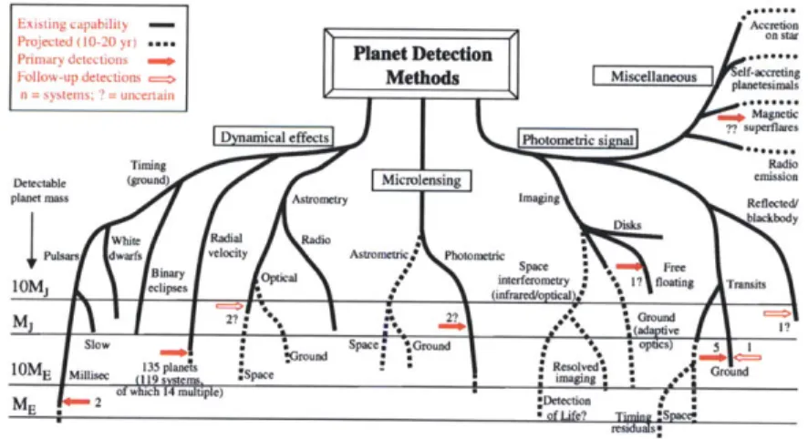
1-3 Exoplanet detection methods and yields as of 2005. . . . . 21

1-4 Exoplanet detection via radial velocity . . . . 24

1-5 A transiting exoplanet configuration and transit light curve. . . . . . 25

1-6 Detecting an exoplanet via transit. . . . . 26

1-7 High precision exoplanetary transit light curves as measured from space. 28 1-8 Changes in midtransit time as a result of a second planet. . . . . 30

1-9 The effect of stellar limb-darkening on the transit light curve of HD 209458b... ... 32

1-10 Transmission spectroscopy of HD 189733b . . . . 33

1-11 Signatures of exoplanetary rings in the transit light curve. . . . . 35

1-12 "Anomalous" velocity in radial velocity measured during transit. . . . 36

2-1 Comparison of the exact and piecewise-linear transit models. . . . . . 48

2-2 Parameter derivatives, as a function of time, for the piecewise-linear and exact model light curves . . . . 51

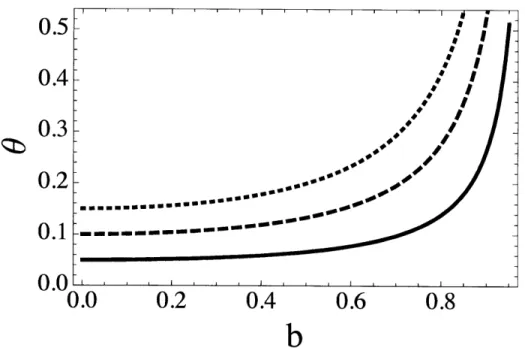
2-3 Dependence of 0 = 1 on depth 6 = r2 _{and normalized impact} param-eter b, for the cases r = 0.05 (solid line), r = 0.1 (dashed line), and r = 0.15 (dotted line). . . . . 54

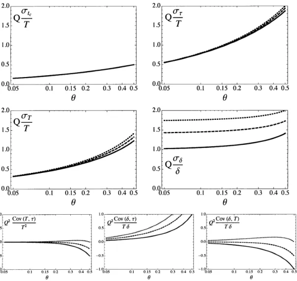
2-4 Standard errors and covariances, as a function of 6 =T /T, for different choices of q. . . . . 55

2-5 Correlations of the piecewise-linear model parameters, as a function of O T/T for different choices of q. Solid line - 7= 0; Dashed line

-7 0.5; Dotted line - = 1. . . . . 57

2-6 Correlations of the piecewise-linear model parameters . . . . 57

2-7 Comparison of the non-zero correlation matrix elements for the exact light-curve model and the piecewise-linear model . . . . 60 2-8 Comparison of the covariance matrix elements for the exact

uniform-source model, linear limb-darkened model, and the piecewise-linear model 61 2-9 Comparison of the analytic correlations and numerically-calculated

correlation matrix elements for a linear limb-darkened light curve . . 63 2-10 Comparison of correlation matrix elements for the piecewise-linear model

and a linear limb-darkened light curve with a redefined depth parameter 64 2-11 Comparison of correlation matrix elements for the piecewise-linear model

and a linear limb-darkened light curve with a redefined depth parameter 64 2-12 Comparison of correlations for various parameter sets that have been

used in the literature. . . . . 68 2-13 Correlations for the parameter set {b, T, r} . . . . 70 2-14 Comparison of the correlations amongst various parameter choices. . 73

3-1 Examples of 1/f^ noise. . . . . 89 3-2 _{Examples of discrete wavelet and scaling functions, for N = 2048. . . 96}

3-3 Illustration of a multiresolution analysis. . . . . 96

3-4 Constructing a simulated transit light curve with correlated noise. 102 3-5 Examples of simulated transit light curves with different ratios a

-rmsr/rmsw between the rms values of the correlated noise component and white noise component. . . . . 103 3-6 Histograms of the number-of-sigma statistic P. for the midtransit time

t1. . . . . 10 5 3-7 Autocorrelation functions of correlated noise. . . . 111

3-8 Accuracy of the truncated time-domain likelihood in estimating mid-transit tim es. . . . . 112 3-9 An example of an autoregressive noise process with complementary

characteristics to a 1/f7 process. . . . . 117 3-10 Simulated transit observations of the "Hot Neptune" GJ 436. . . . . . 120 3-11 Transit timing variations estimated from simulated transit observations

of GJ 436b. ... ... 121

3-12 Wavelet analysis of a single simulated transit light curve. . . . . 123 3-13 Results of parameter estimation for the simulated light curve of Fig. 3-12.124 3-14 Isolating the correlated component. . . . . 125 4-1 NICMOS photometry (1.1-2.0 pm) of HD 149026b of 4 transits, with

interruptions due to Earth occultations . . . . 141 4-2 Illustration of inter-orbital variations of the spectral trace. . . . . 142 4-3 Histograms of the residuals between the data and the best-fitting model.

145

4-4 Assessment of correlated noise. . . . . 145 4-5 NICMOS photometry (1.1-2.0 pm) of 4 transits of HD 149026b, after

correcting for systematic effects. . . . . 147 4-6 NICMOS transit light curve (1.1-2.0 pm) of HD 149026b . . . . 148 4-7 Comparison of the best available transit light curves of HD 149026. 149 4-8 Isolation of the intra-orbital variations. . . . . 152 4-9 Results for the limb-darkening parameters ui and . . . . 153 4-10 Stellar-evolutionary model isochrones, from the Yonsei-Yale series by

Y i et al. (2001). . . . . 155 4-11 The planet-to-star area ratio, (R,/R,)2_{, as a function of observing}

wavelength . . . . 160

4-12 Transit-timing variations for HD 149026b. . . . . 161 4-13 Illustration of wavelength-dependent absorption. . . . . 164

4-14 Measured transit light curves of HD 149026b at the same transit epoch over twenty-four uniformly distributed wavelength channels covering the NICMOS G141 1.1 - 2.0 pm bandpass. . . . 169 4-15 The transmission spectrum from 1.1 - 2.0 pm for HD 149026b. . . . . 170 5-1 _{Geometrical configuration for the transit of an ellipsoidal planet across}

a spherical star. . . . 189 5-2 Quasi-Monte Carlo integration of the non-trivial component of the

to-tal flux deficit for the stellar transit of an oblate planet. . . . 194 5-3 Signals of oblateness for hypothetical transit light curve models of HD

189733b... ₁₉₇

5-4 Light curves from seven Spitzer observations of HD 189733b. . . . 199 5-5 Systematic corrected transit light curves of seven Spitzer observations

of HD 189733b. . . . 202 5-6 Combined transit light curve and residuals of seven Spitzer observations

of H D 189733.. _{. . . 203} 5-7 Oblateness constraints for HD 189733b based upon seven Spitzer

tran-sit observations. . . . 207 5-8 Posterior distributions for the rotational period, Prot, and the second

spherical moment of the mass distribution, J2, of HD 189733b based

upon seven Spitzer transit observations. . . . 208 5-9 Theoretical spin precession periods and transit depth variations for HD

189733b... 213

5-10 Simulated transit light curves for an oblate HD 80606b. . . . 214 5-11 Measuring oblateness in a simulated transit light curve for HD 80606b. 215 A-i An elliptical annular sector. . . . 222

List of Tables

2.1 Table of partial derivatives of the piecewise-linear light curve F', in the five parameters {pi} = {tc, T, T, 6, fo}. The intervals It - tc| <

T/2-T/2, T/2 -- /2 < |t -tc| < T/2+T/2, and |t -te| > T/2+T/2

correspond to totality, ingress/egress, and out of transit respectively. . 50

2.2 Table of transit quantities and associated variances . . . . 67

2.3 Covariance matrix elements for use in Table (2.2). . . . . 68

3.1 Estimates of mid-transit time, te, from data with known noise properties106 3.2 Effect of time sampling on the white analysis . . . . 107

3.3 Estimates of te from data with unknown noise properties . . . . 108

3.4 Estimates of te from data with unknown noise properties . . . . 109

3.5 Estimates of tc from data with autoregressive correlated noise . . . . 116

3.6 Linear fits to estimated midtransit times . . . . 119

4.1 System Parameters of HD 149026. . . . . 172

4.2 Mid-transit times, based on the NICMOS data. . . . . 172

5.1 Solar System planet parameters . . . . 185 5.2 Parameters for HD 189733b and the combined Spitzer transit light curve205

Chapter 1

Introduction

One of the burning questions of astronomy deals with frequency of planet-like bodies in the galaxy which belong to stars other than the Sun.

- Otto Struve (1952)

In looking over the long history of human science from time immemo-rial to our own times, it is impossible to overestimate the role played in it

by the phenomena of eclipses of the celestial bodies both within our solar

system as well in the stellar universe at large.

- Zdenek Kopal (1990)

1.1

Planets near and far

1.1.1

Our own Solar System

It was realized early in recorded history that, looking at the night sky, amongst the "fixed" stars in the "heavenly firmament" a group of wandering objects traced repeatable paths on the celestial sphere. These planets (literally "wanderers" in Greek), initially regarded as the physical manifestations of powerful mythological gods, were, in fact, worlds in many ways like the Earth, likely arriving from the same evolutionary process that gave birth to our common stellar host Sol. Upon closer inspection, famously first by Galileo's pioneering work identifying the moons of

Jupiter and the phases of Venus, each planet is found to be remarkably distinct from its siblings. In order of increasing semi-major orbital distance, the interior planets Mercury, Venus, Earth and Mars are small rocky worlds, while Jupiter and Saturn are gas giants lacking any substantial rocky core, and finally, Uranus and Neptune are "ice giants" having mean densities lying in between that of the terrestrial and Jovian worlds [see Carrol & Ostlie (2006) Part III for an excellent review of the Solar System]1. Most planets are also accompanied by a collection of natural satellites (and now even artificial satellites) in the form of moons and diffuse rings. Each planetary system is, in its own right, a complicated and rich dynamical collection of gravitationally bound objects. Humanity has gone to extensive investigative lengths to classify, explain, or simply photograph these worlds with complex (and expensive) experiments including a series of manned (in the case of the Moon) and unmanned spacecraft missions right to the source. We work towards both an explanation of the planets in isolation from the remaining planets and as a Solar System as a whole. In particular, we ask the questions that relate most to our own planet's existence: how do these other planets (and moons) compare to Earth? Is Earth an atypical object in this small sample? Could other planets in our Solar System harbor their own form of life? Intelligent life? The final two questions are likely to induce the strongest inquisitive response from even the most uninformed, given that the answers to these questions will no doubt shed light on our very relevance in the universe.

1.1.2

Extrasolar planets:

Planets outside our own Solar System

The most natural question following the above line of questioning is, given the pre-ponderance of Sun-like stars in our own galaxy, how many planets are there that orbit stars other than our Sun? And assuming this answer is non-zero (yes, it is) are there multiple planets orbiting a single star other than our Sun? Going further, we may ask: How many of these extrasolar systems contain Jovian-type planets? Ice

1_{In August 2008, the International Astronomical Union (IAU) defined the term "planet."}

giant-like? Terrestrial planets? Earth-like? Do these planets have rings? Moons? Atmospheres? Life? We as a research community, at the time of writing, have at least some idea of the answers to many of these questions.

Extrasolar planets, or exoplanets in the parlance of the field, number in the hun-dreds (353, as of July 2009). However, prior to 1995 [and the discovery of 51 Peg b by Mayor & Queloz (1995)], we only knew of the 9 Solar System planets (reduced now to 8, see footnote). The expectation for discovery was in place, as suggested in the short note by Struve (1952) in which the possibility of detection was first appreciated. The next section reviews Struve's recommended method of detection and other tech-niques, including the transit. Since 1995, however, the pace of discovery has steadily grown. In Figure (1-1) we show the number of exoplanets discovered by year, since 1995. In particular, the pace of discovery of planets that transit their stellar host (see

§

1.2.2 below) has recently reached a doubling time that is less than one year [Charbonneau et al. (2009)].

As the number of exoplanets with precisely measured properties (see

§

1.3) grows, we find ourselves on the frontier of a realm in which statistically meaningful general-izations may be drawn of planets as a whole. Homogeneous analyses of these precisely characterized systems (Torres et al. 2008, Southworth 2008) demonstrate trends in the parameter space [see Figure (1-2)] allowing us to reach somewhat-informed con-clusions about the population of exoplanets yet to be discovered. However, in many ways, we are still very far from a complete understanding. But the prospects look good: initial estimates based upon our current sample of exoplanets imply that nearly 6% of stars harbor at least one giant planet within 4 AU. With this statistic as mo-tivation, we need to (1) find more planets and (2), in the pursuit of a fundamental theory of planets, characterize these objects as accurately as possible.

While the work presented in this Thesis is geared more to the goal of point (2), we review the techniques relating to exoplanet discovery in the next section.

so-Transiting exoplanets

- All exoplonets

l's

2L0hIIIIE

Figure 1-1 Exoplanet detections and organized by J. Schneider. 2.0 1.5 M 1.0 0.5 1 2 3 Orbital period (days)

totals by year. Data from exoplanets.eu,

0.0 0 2.0 -1.0 4 5 1 2 3 4

Orbital period (days)

Class I

Class II

1000 1500 2000 2500

T., (K)

Figure 1-2 Exoplanet trends and correlations. Plotted are parameters determined in the homogeneous analysis by Torres et al. (2008) for a selection of exoplanets. In particular, correlations between exoplanet radius, R,, mass M,, orbital period P, surface gravity gp and equilibrium temperature Te are shown. Figures by Torres et al. (2008); refer to their paper for details.

(a) -U, 0".,~)

(1,)

. . . .

mad

I IM

=0

3001

2M 2003 IM

IN-1.2

_{Detecting extrasolar planets}

We must actually find exoplanets prior to attempting accurate parameter estimation. A number of techniques exist to detect exoplanets and may be organized into the following categories: (1) photometric (transits), (2) dynamical (primarily radial ve-locity, but also astrometry and timing), (3) microlensing, (4) direct imaging and (5) others (Perryman et al. 2005). Figure (1-3) organizes these detection techniques in a graphical manner indicating planetary mass detection limits. While this diagram is out-dated and statistics have changed [only 4 years old and missing hundreds of exoplanets that have been discovered since! See Fig. (1-1)], the top three techniques by total yield remain the same and in the following order: radial velocity (327 plan-ets), transits (59 planets) and microlensing (7 planets). Each of these techniques has their respective advantages and disadvantages in terms of detection capability. We will show, in

§

_{1.3, that while transit detection may be considered inferior to (or}

incomplete without) radial velocity detection, transit characterization of exoplanets is unrivaled. We will briefly describe the radial velocity technique before moving onto detection via transit. See Perryman et al. (2005) and the references therein for a discussion of alternate detection techniques (including microlensing).

Figure 1-3 Exoplanet detection methods and yields as of 2005. Figure by Perryman et al. (2005).

1.2.1

Detection via radial velocity

The well-studied and understood two-body gravitational problem [see, e.g., Carrol & Ostlie (2006)] includes the basic prediction that each massive object moves in an elliptical orbit about the common center of mass. As a result, the velocity of the objects (in the center-of-mass frame, without loss of generality) oscillates at the orbital period, P, and each with a unique amplitude, Ki, that depends on a formula involving the masses. In particular, if one of the objects is a star and the other is an unseen planet, we may infer the existence of the less massive component by monitoring the periodic signature on the stellar component's velocity [this was first appreciated by Struve (1952)]. We may measure the component of the velocity along the line of sight by using the principle of Doppler spectroscopy [see, for example, Butler et al. (1996)]. Here, information regarding the relative velocity along the radial direction is encoded in the spectral lines of the stellar spectrum as a result of Doppler frequency-shifting. One may obtain better than 3 m s-1 _{precision on the}

measurement of radial-velocity with a proper calibration of rest wavelengths of the spectral lines (and other instrumental calibrations, Butler et al. 1996). We may fit a model to the collection of radial velocity measurements to determine orbital parameters and masses. For a single planetary component, a simple Keplerian model will suffice. In particular, we may solve for the mass of the planetary object, M, and orbital semi-major axis a,

Msini _{MP sin i} = _- KV1- _KVI27rG e2 P (M, + M, sin i)2 1/311 _(I

a 3 M* + M, sin i P 2

___ ₀ =M ,(1.2)

1 AU me yr '

in terms of the stellar mass M* and the inclination angle i of the orbital plane to the observational plane, where K is the amplitude of the radial velocity, e is the orbital eccentricity and P is the orbital period. The parameters K, e and P may be measured directly from the radial velocity data [e.g. Butler et al. 2006 and see Fig. (1-4)] . The stellar mass M* may be precisely estimated via spectral identification, for example.

The inclination i is an unknown parameter degenerate with the planetary mass; we therefore can only estimate M, sin i < Mp.

The radial velocity exoplanet detection technique has several advantages. While the mass is degenerate with inclination i, only parallel orbital plane configurations

(i = 00) yield a non-detection. Current radial velocity exoplanet detection technology allows for the detection of exoplanet's with masses equal to a few times an Earth mass or less (the so-called "Super Earths"). Examples include the three orbiting HD 40307, with masses 4.2, 6.9, and 9.2 MD, found by Mayor et al. (2009) with the HARPS spectrograph (Pepe et al. 2002) at the La Silla Observatory in Chile. Currently, radial velocity is the detection method best suited to the detection of Earth-like analogs.

Exoplanet detection via radial velocity is unfortunately very costly in both dollars and time. Radial velocity measurements must uniformly sample the orbital phase in order to precisely measure orbital parameters of the unknown planetary component. For a Jupiter analog (5 AU from the Sun making one orbit every 12 years), it would take several years of observations to make detection possible. Radial velocity surveys are capable of tremendous yield for short-period giant exoplanets [i.e., 51 Peg b-like, Mayor & Queloz (1995)]. However, given the limited information that may be derived about the exoplanet and its orbit (namely M, sin i, e, P), radial velocity

characterization of short-period giants has quickly diminishing returns.

1.2.2

Detection via transit

If the orbital plane of the exoplanetary system were to lie in the plane perpendicular

to our observational plane (i = 90'), then the exoplanet will periodically pass in

between its star and our telescopes. This fortunate configuration results in what is referred to as a transit2. The observational effect of transit is that the obscured star is perceived to experience a systematic decrease in total flux. For a planet in a stable

2

The obscuration of one celestial body by another is referred to as an eclipse, in general, and is the subject of the general mathematical theory of Kopal et al. (1990) or as found in Mandel & Agol (2002). In practice, the word eclipse is reserved for the situation common to eclipsing stellar binaries where the two eclipsing components are of equal radial extent. If the object passing in front of the other from our perspective is significantly smaller (larger) than its companion then the eclipse is referred to as a transit (occultation).

- HIRES -+CORAL!IE _oELOD1E ++ + + S .+ + + 4.4 -14.7 , ,,M, , oo . 4.2 LI ** + > 14.8 + + ++ + S +.+ + 3.6 -14.9 _____________________ 0.0 0.2 0.4 0.6 0.8 1.0 0.0 0.5 1.0 Phase

Figure 1-4 Exoplanet detection via radial velocity. The left panel shows the radial velocity signature of the exoplanet HD 209458b on HD 209458 [Figure by Mazeh et al. (2000)]. The right panel shows the radial velocity signature of HD 80606b on HD 80606 [Figure by Naef et al. (2001)]. The sharp features in the radial velocity curve for HD 80606 are as a result of the high orbital eccentricity of HD 80606b. See

§

1.2.1 for details.

Keplerian orbit, the size and duration of the flux deficit are fixed. Additionally, the time between subsequent events is constant (equal to the orbital period, P). When the exoplanet passes behind the star from our perspective (so-called occultation), an analogous drop in total flux is observed, this time owing to the stellar obscuration of the planetary flux. The transit configuration is illustrated in Fig. (1-5) along with the "transit light curve," the dynamical curve describing the total flux measured for star and planet.

The depth J of the transit is related to the fraction of area obscured by the exoplanet and, therefore, is related to the ratio of the radii of planet and star (see Chapter 5 for an alternate possibility). The spacing of subsequent transit events is directly related to the orbital period P. Thus, a photometric survey program can establish the existence of a transiting body with the observation of repeated, uniform drops in flux from a star. This was first realized in the same note as discussed above by Struve (1952) and considered further by Rosenblatt (1971) and Borucki & Summers (1984).

For a Jupiter sized planet transiting a Sun-like star, the expected deficit in flux, 6, should be about 1%. This precision may obtained for bright stars with modest

Flux

Time

Figure 1-5 A transiting exoplanet configuration and transit light curve. Figure courtesy of J. Winn. The transit portion of the light curve can be minimally described by a depth, 6, transit duration, T and ingress or egress duration T. See

§

1.3 for details.

telescopes and imaging equipment. For this reason, a number of relatively cheap pho-tometric surveys have sprung up for the purpose of exoplanet transit detection. See Perryman et al. (2005) for a comprehensive list of ground and space-based photo-metric surveys. The most "famous" of this collection are those with largest harvests. From the ground: OGLE [the first such survey, 7 planets, Udalski (2007)], TrES [4 planets, Alonso et al. (2004a)], XO [5 planets , McCullough et al. (2005)], HATNet

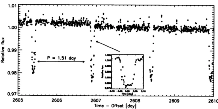
[12 planets, Bakos et al. (2007)] and WASP [15 planets, Pollacco et al. (2006)]; from space: CoRoT [7 planets, Baglin et al. (2003), see Fig. (1-6)]. Recently, the space-based transit-survey mission Kepler (Borucki et al. 2009) was launched and has the potential for most transit-discoveries, likely out-pacing the radial velocity discovery rate.

One negative cost of transit discovery is based upon simple probability: given that planetary systems in the galaxy are likely to be randomly oriented, it is improbable to find a significant number of exoplanets whose chance alignment allows a transit from our perspective. We can quantify this probability via geometric analysis. Namely, the probability of observing a transit of a particular exoplanet is equal to the ratio of the solid angle in which the planet will be seen to transit and the total available

1.01 -.00. . nr -- s. A * M& . 0.99 P2=P 1.51 day : _-. 0.98 *2 0.97 . . . . . . - - - -2605 2606 2607 2608 2609 2610

Time - Offset [doy]

Figure 1-6 Detecting an exoplanet via transit. Plotted here is discovery data showing the transit of CoRoT-1b in successive transit epochs [Baglin et al. (2003)].

solid angle (47r). The probability of transit, Ptransit, is, therefore, mainly dependent

on the ratio of the semi-major axis a and stellar radius R, as

Ptrnst -. 0451 AU) (R, + R, 1I + e cos(7r/2 - w)(13

Ptransit =0.0045 w) _(1.3)R

(a 1- e2

where e and w are the eccentricity and argument of periastron for the orbit and our line-of-sight, respectively (Charbonneau et al. 2007). For an Earth analog, the probability of transit is therefore Ptransit ~ 0.45%. On the other hand, a

Jupiter-sized planet orbiting a Sun-like star at 0.05 AU has a more palatable 10% transit probability. Before the identification of 51 Peg b-like "Hot Jupiters," or short-period gas giants, it was assumed, based upon our experience with our own Solar System, that transit surveys would be a low yield affair. Post 1995, as radial velocity survey yields implicated that fully 1% of nearby sun-like stars hosted these "Hot Jupiters," the interest in photometric surveys grew (Horne 2003).

The expectations from the research community for transit surveys were tremen-dous, with an anticipation of ~ 10 "Hot Jupiter" planets discovered per month for surveys with WASP-like characteristics (Horne 2003). That the current generation of surveys has not reached this rate is a testament to the additional difficulties as-sociated with being able to identify transits in data and definitively declaring a flux decrement to be planetary in nature. The former problem is related to the discussion

in Chapter 3 and is, in part, related to the fact that time-correlated noise can affect the exoplanet detection threshold, reducing the number of detected planets based on a uncorrelated assumption (see, Chapter 3 and Pont et al. 2006). The latter prob-lem arises because, while radial velocity detection can make some statement about the mass of the secondary object, a transit light curve only can measure fractional obscuration. The signal interpreted as a planetary transit could be as a result of grazing eclipsing binaries, the transit of a brown dwarf across a giant star, the blend-ing of light from a triple star system in which two components are transitblend-ing, and more (see, e.g., Alonso et al. 2004b, O'Donovan et al. 2007). Such confusion can be eliminated by a subsequent radial-velocity follow-up of the exoplanet candidate host thereby constraining the planetary mass M,. Here, since the planet is seen to transit,

i ~ 90' and the degeneracy between planetary mass and inclination is broken.

Even in the face of these difficulties, modern transit surveys survive by collecting light curves for a large number stars. Acquiring large numbers of stars is accomplished rather easily for a photometric survey covering a significant portion of the sky (wide) and/or capable of detecting very faint stars (deep).

1.3

Characterizing extrasolar planets that transit

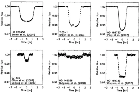
While the detection of exoplanets via transit can be a profitable endeavor, the real power of transit light curve analysis lies in exoplanet characterization. The infor-mation encoded in the transit light curve is capable of uniquely determining a large number of exoplanet observables. In this section of the introduction, we quickly re-view the transit light curve as a tool for precise exoplanet analysis. Prior to diving into the details, it is useful to carefully study the model light curve in Fig. (1-5) and the "gallery" of real, space-based transit light curve data in Figure (1-7).

-3 -2 -1 0 1 2 3 Time [hr] 1.00 0.99-0.98 GJ 436 Gillon et o1. (2007) 0.97 ein et (2007 -3 -2 -1 0 1 2 3 Time [hr) 1.00 V ft. 0.99 0.98 -TrES- 1

0.97 Brown et al., in prep. -3 -2 -1 0 1 2 3 Time [hr] 1.00 0.99 0.98 HO 149026 0.97 Nutzman et al. (2008) -3 -2 -1 0 1 2 3 Time [hr] 1.00 0.99 0.98-HO 189733 0.97 Pont et al. (2007) -3 -2 -1 0 1 2 3 Time [hr] 1.00 0.99-0.98 -HO 189733 0.97 Knutson et 1. (2007) -3 -2 -1 0 1 2 3 Time [hr)

Figure 1-7 High precision exoplanetary transit light Figures by Winn (2009).

curves as measured from space.

1.3.1

The exoplanetary transit light curve:

From top to bottom

The effect of a transit of an exoplanet across the face of its star is most simply described by the following equation for F, the total flux measured for the combined exoplanet-host system

F = F,(planet)

+

F,(star) - F,(planet

n

star)

F,(planet

n

star)

if planet nearer if star nearer

where F,(Q), F,(Q), are the integrated flux of planet and star over the integration region Q. We have used the shorthand "planet," "star," or "planet

n

star" to indicate whether the integration region Q is over the sky-projected planet surface, stellar surface or the intersection of the two. To first order, the sky-projected shape of exoplanet and star are disks with radius R, and R, respectively (see Chapter 5 for an alternative model).

Timescales and observables

The total flux F depends upon time, t. Most importantly, given is in orbit around the star, planet

n

star is a function of time. duration of the transit, T, (when planet

n

star

#

0)

scales with

P, as

T ~- R P

a 7r

that the exoplanet In particular, the the orbital period,

(1.5)

while the duration of ingress or egress, T, (for which planet

n

star

#

planet) scales as

a 7r (1.6)

If we use Kepler's third law [Eqn. (1.2)], we may write T in a more suggestive form

( P

-1_/3

po)

(1.7)

It is therefore feasible to utilize the duration of the transit (or occultation) to make estimates of the mean stellar density, p, [Perryman et al. 2005, Seager & Mallen-Ornelas 2003]. These precise density estimates may then be used in combination with stellar evolution models to constrain properties of star and planet (see Chapter 4). Again utilizing Kepler's third and also the radial velocity-determined mass M, in Eqn. (1.1), we may write T in the more suggestive form

T f 24

1I yr)

gp -1/2 K 1/2

gJ 1 m/s min. (1.8)

It is therefore also feasible to utilize the duration of transit ingress to make estimates of the planetary surface gravity, gp [Southworth et al. (2007)].

Timing and additional, unseen planets

If we assume the exoplanet follows a Keplerian orbit around its star then the time between two successive transits Atc should be equal to the orbital period P. However,

p 1/3

if the planet's orbit is perturbed by the gravitational tug of other unseen planets then Atc = P

+

6P(t). The perturbation to the linear model, 6P(t), is a function of the

mass of the unseen object (Holman & Murray 2005, Agol et al. 2005). It is therefore possible to detect additional planets and their masses from an analysis of a collection of midtransit times [see Fig. (1-8)]. It is important to note that midtransit times are acutely affected by time-correlated noise in the data; special care must therefore be taken to ensure these times are accurate for physical interpretation (see Chapter 3).

HD209458b (P = 3.5248 d, e = 0.025) 30 P2' 99.8d e = 0.7 20 10 0 10 --10 30 P₂ = 28. d e₂ 0.3 20 10 0 -o -10 -20 20 20040060 S10 ~ 0 -10 20UL 0 200 400 600 time (days)

Figure 1-8 Changes in midtransit time as a result of a second planet. This figure, by Holman & Murray (2005), presents variation in the time of midtransit (between successive transits) of HD 209458b in response to gravitation perturbations from a second planet with orbital period P2 and orbital eccentricity e2.

Transit or occultation depth: Stellar and exoplanetary atmospheres

The relative transit depth, 6, is given by the normalized form of Eqn. (1.4) at maxi-mum obscuration (planet

n

star = planet),

Fp(planet) + F,(star) - F,(planet)

F(planet) + F,(star)

F,(planet) _(1.9)

F(planet) + F,(star) 30

We have assumed that the stellar and planetary fluxes are constant, however, stellar variability can have a significant effect on the transit light curve [see, e.g., Czela et al. (2009), Silva (2003)]. If, for the moment, we assume the stellar brightness profile

I,(r, 6) is constant then

R,2 F(planet) (1.10)

R* F,(star)

If we assume further the flux due to the planet, F,, is negligible compared to that of the star then 6 _ (R,/R,)2. Thus, the transit depth places a precise constraint on

the exoplanetary radius.

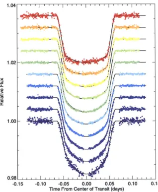
Constant stellar brightness profiles are reasonable approximations at mid-infrared and longer wavelengths (see Chapter 5), however, in general, stellar limb-darkening suppresses flux at the stellar disk edges. The effect of the limb-darkening is strongly wavelength dependent and significantly affects the shape of the transit light curve at optical wavelengths [see Figs. (1-7,1-9)]. Limb-darkening tends to round the otherwise boxy transit light curve profile, working to confuse accurate estimation of transit parameters (see Chapter 2). On the other hand, exoplanetary transit light curves provide valuable information about limb-darkening profiles [such as those proposed by Claret (2000)] for stars other than our Sun (Knutson et al. 2007a).

So far, we have regarded the planetary radius, R,, as independent of how we observe the transit. This is not generally true. In particular, the radial extent of the planet depends on the wavelength of observation, so that R, = R,(A). The reason

for this dependence is simple: what we as the observer perceive as the radial extent of the exoplanet is determined by the height in the exoplanet atmosphere at which the optical depth for stellar light passing through the atmosphere on its way to us reaches unity, say. This height, z, is dependent on the structure of the atmosphere, the sources of opacity [rotation-vibrational molecular absorption, for example, see Fig. (1-10)], and the wavelength A of our observation (Seager & Sasselov 2000, Brown 2001, Hubbard et al. 2001, Hui & Seager 2002 and Chapter 4). By observing transits and determining transit depths at multiple wavelengths, we may form an absorption

spectrum of the planetary atmosphere. This technique, as executed by Swain et al. (2008) and illustrated in Fig. (1-10), is often referred to as transmission spectroscopy.

-0.15 -0.10 -0.05 0.00 0.05 Time From Center of Transit (days)

0.10 0.15

Figure 1-9 The effect of stellar limb-darkening on the transit light curve of HD 209458b. In this figure by Knutson et al. (2007), transit light curve data is shown for HD 209458b in wavelength bands spanning from 293 to 1019 nm. The curvature in each light curve is as a result of wavelength dependent stellar limb-darkening.

While we, in this Thesis, are concerned mainly with the transit portion of the total light curve [Eqn. (1.4)], an observation at occultation is extremely useful in

constraining the atmosphere of the exoplanet. The occultation depth, 6, may be derived in an analogous fashion to Eqn. (1.9) as

=1 - F,(planet) + F,(star) - F,(planet)

F,(planet) + F,(star) F, (star) = 1 -F,(planet) + F,(star) (1. 11) F,(planet) F,(star)

If we again assume that the brightness profile of both planet and star are constant

.... ...

_ Binned model, water + methane

Binned model, water + methane + ammonia

+ Binned model, water + methane + CO

A Observations

2.45

--20

2.35

--Model, water

Model, water + methane

2.30 I . . . I

1.6 1.8 2.0 2.2 2.4

Wavelength (pm)

Figure 1-10 Transmission spectroscopy of HD 189733b. This figure by Swain et al. (2008) plots the wavelength-dependent transit depth for the exoplanet HD 189733b. The shape of the spectrum suggests the presence of methane in the exoplanet atmo-sphere.

then

0 ~. -- -2 (1.12)

(R* I*

where the ratio of the planetary and stellar intensities I,/I, is, to first order, related to the black-body temperature of planet and star. For an observation in the infrared,

I,/II ~ T,/T . A measurement of occultation depth can, therefore, constrain the temperature of the photosphere of the exoplanet [see, for example, Harrington et al.

(2007)].

The thermal emission from the exoplanetary photosphere may be non-uniform across its surface. Thus, as the planet rotates to show different faces while it moves through its orbit, we will measure a time-varying total flux, F+(star) + F,(planet). By measuring this light curve (the so-called "phase function") we may learn how heat is transported through and redistributed throughout the exoplanet atmosphere. If the rotational period is known precisely, this phase function may be inverted into a temperature map of the planetary photosphere [as was done for HD 189733b, see Knutson et al. (2007b)].

At visible wavelengths, stellar light reflected off the planetary surface (by clouds, for example) is the dominant contribution to the occultation depth, whereby

oo0~ a _(1.13)

where a is the geometric albedo of the exoplanet (e.g., Seager 2008). By first measur-ing the quantity R,/a durmeasur-ing transit, a measurement of occultation depth in optical wavelengths would yield the albedo a.

Moons, Rings and Oblateness

While we have so far assumed the exoplanet is circular in projection, perturbations to the obscuring shape are possible, if not likely. If, for example, the exoplanet has close gravitationally bound companions, such as moons or rings, it is likely they will induce a non-trivial effect on the transit light curve. Even with no companions present, the exoplanet itself is likely to be non-spherical, as is the case with Solar System planets

(Murray & Dermott 2000).

Moons present the most obvious perturbation, contributing to the total flux deficit as an additional transit on top of the transit of the exoplanet. Time varying effects in the photometry may help to constrain the exomoon mass and orbital period. Cur-rently no transit data support the presence of an exomoon around any of the transiting planets [see, for example, Pont et al. (2007)]. Exomoons may also be detected by identifying the signature of their gravitational effect on their planetary host from anomalies in a collection of midtransit times or in the time variability of transit durations (Kipping 2000).

Rings present a subtler effect on the transit light curve, depending on the orien-tation of the rings in the sky plane and the level of extinction due to ring particles [Barnes & Fortney 2004, Ohta et al. 2009, see Figure (1-11)].

The shape of the exoplanet, most notably oblateness owing to rigid-body rotation of the bulk (see Chapter 5), is in principle measurable from the transit light curve. The effect is most evident during the phases of ingress and egress. With a measurement

of oblateness, it is possible to constrain the planet's rotation period, its internal constitution and possible evolutionary histories (see Chapter 5).

0.0010 0.0005 0.0000 -0.0005 -0.0010 0.0010 0.0005 0.0000 -0.0005 -0.0010 0.0010 0.0005 0.0000 -0.0005 -0.0010 -5 0 5

Time from midtransit (hours)

Figure 1-11 Signatures of exoplanetary rings in the transit light curve. Figure by Barnes & Fortney (2004).

Transits in radial velocity

The transit, when observed with Doppler spectroscopy (as used for detection in

§

1.2.1), appears as an "anomalous" perturbation to the radial velocity of the stellar host [see Fig. (1-12)]. This so-called Rossiter-McLaughlin effect is as a result of the obscuring exoplanet covering a portion of the receding (approaching) half of the ro-tating stellar disk inducing an excess of "red" ("blue") Doppler-shifted photons. By measuring the radial velocity at transit, it is therefore possible to measure the sky projection of the angle between the spin axis of the star and that of the exoplanetary orbit (Gaudi & Winn 2007). This angle can be used to constrain possible dynamical scenarios involving additional planets in the stellar system [see, for example, Fabrycky & Tremaine (2007)].

-200 E 100-. 0 -100--200* --1.0 -0.5 0.0 0.5 1.0 Days since mid-transit

100 . 50 E 0 ... .--- -- ... -.. ...-- -- .. ..-.. -- ...- .. -- ----. .. -50 -0 0 X -0.10 -0.05 0.00 0.05 0.10 Davs since mid-transit

Figure 1-12 "Anomalous" velocity in radial velocity measured during transit. This figure showing the Rossiter-McLaughlin effect for HD 189733b is by Winn et al.

(2006). See

§

1.3.1 for details.

1.4

Thesis overview

As we have attempted to make clear, the light curve of an exoplanetary transit can be used to estimate the planetary radius and other parameters of interest. Because accu-rate parameter estimation is a non-analytic and computationally intensive problem, it is often useful to have analytic approximations for the parameters as well as their uncertainties and covariances. In Chapter 2, we give such formulas, for the case of an exoplanet transiting a star with a uniform brightness distribution. We also assess the advantages of some relatively uncorrelated parameter sets for fitting actual data. When limb darkening is significant, our parameter sets are still useful, although our analytic formulas underpredict the covariances and uncertainties.

We consider, in Chapter 3, the problem of fitting a parametric model to time-series data that are afflicted by correlated noise. The noise is represented by a sum of two stationary Gaussian processes: one that is uncorrelated in time, and another that has a power spectral density varying as 1/f. We present an accurate and fast [O(N)] algorithm for parameter estimation based on computing the likelihood in a wavelet

basis. The method is illustrated and tested using simulated time-series photometry of exoplanetary transits, with particular attention to estimating the midtransit time

(see

§

1.3.1). We compare our method to two other methods that have been used in the literature, the time-averaging method and the residual-permutation method. The algorithm presented in this chapter generally gives more accurate results for midtransit times and truer estimates of their uncertainties.

The transiting exoplanet HD 149026b is an important case for theories of planet formation and planetary structure, because the planet's relatively small size has been interpreted as evidence for a highly metal-enriched composition. We present, in Chap-ter 4, observations of 4 transits with the Near Infrared Camera and Multi-Object Spec-trometer on the Hubble Space Telescope within a wavelength range of 1.1-2.0 Pm. Analysis of the light curve gives the most precise estimate yet of the stellar mean density (see

§

1.3.1), p, = 0.497- g cm--3. By requiring agreement between the observed stellar properties (including p*) and stellar evolutionary models, we refine the estimate of the stellar radius: R* = 1.541ii84 Ro. We also find a deeper transit than has been measured at optical and mid-infrared wavelengths. Taken together, these findings imply a planetary radius of R, = 0.813ij.2 Raup, which is larger than earlier estimates. Models of the planetary interior still require a metal-enriched composition, although the required degree of metal enrichment is reduced. It is also possible that the deeper NICMOS transit is caused by wavelength-dependent absorp-tion by constituents in the planet's atmosphere (see

§

1.3.1), although simple model atmospheres do not predict this effect to be strong enough to account for the dis-crepancy. We use the 4 newly-measured transit times to compute a refined transit ephemeris.

Finally, in Chapter 5, we place empirical constraints on the oblateness (see

§

1.3.1) of the "Hot Jupiter" HD 189733b by completing a careful analysis of 7 transits ob-served with the InfraRed Array Camera (IRAC) onboard the Spitzer Space Telescope. We rule out, at 95% confidence, oblateness similar to that of Saturn at all or, for that of Jupiter, at most obliquities. By assuming the oblateness to be as a result of rigid-body rotation, we place constraints on the rotational period of the planet. In

particular, we find that HD 189733b is rotating slower than once every 21 hours at 95% confidence. We also consider the detection of oblateness for the highly eccentric transiting exoplanet HD 80606b. The algorithm developed to quickly calculate the transit light curve of an oblate exoplanet is described in depth.

Bibliography

Agol, E., Steffen, J., Sari, R., & Clarkson, W. 2005, MNRAS, 359, 567 Alonso, R., et al. 2004a, ApJ, 613, L153

Alonso, R., Deeg, H. J., Brown, T. M., & Belmonte, J. A. 2004b, Stellar Structure and Habitable Planet Finding, 538, 255

Baglin, A. 2003, Advances in Space Research, 31, 345 Bakos, G. A., et al. 2007, ApJ, 656, 552

Barnes, J. W., & Fortney, J. J. 2004, ApJ, 616, 1193 Borucki, W., et al. 2009, IAU Symposium, 253, 289 Brown, T. M. 2001, ApJ, 553, 1006

Butler, R. P., et al. 2006, ApJ, 646, 505

Carroll, B. W., & Ostlie, D. A. 2006, Institute for Mathematics and Its Applications, Charbonneau, D., Brown, T. M., Burrows, A., & Laughlin, G. 2007, Protostars and

Planets V, 701

Claret, A. 2000, A&A, 363, 1081

Czesla, S., Huber, K. F., Wolter, U., Schrter, S., & Schmitt, J. H. M. M. 2009, arXiv:0906.3604

Gaudi, B. S., & Winn, J. N. 2007, ApJ, 655, 550 Harrington, J., Luszcz, S., Seager, S., Deming, D.,

Holman, M. J., & Murray, N. W. 2005, Science, 307, 1288

Horne, K. 2003, Scientific Frontiers in Research on Extrasolar Planets, 294, 361 Hubbard, W. B., Fortney, J. J., Lunine, J. I., Burrows, A., Sudarsky, D.,

Hui, L., & Seager, S. 2002, ApJ, 572, 540 Kipping, D. M. 2009, MNRAS, 392, 181

Knutson, H. A., Charbonneau, D., Noyes, R. W., Brown, T. M., & Gilliland, R. L. 2007a, ApJ, 655, 564

Knutson, H. A., et al. 2007b, Nature, 447, 183

Kopal, Z. 1990, Dordrecht, Netherlands, Kluwer Academic Publishers, 1990, 163 p., Mayor, M., et al. 2009, A&A, 493, 639

Mazeh, T., et al. 2000, ApJ, 532, L55

McCullough, P. R., Stys, J. E., Valenti, J. A., Fleming, S. W., Janes, K. A., & Heasley, J. N. 2005, PASP, 117, 783

Murray, C. D., & Dermott, S. F. 2000, Solar System Dynamics, by C.D. Murray and S.F. Dermott. Cambridge, UK: Cambridge University Press, 2000.,

Naef, D., et al. 2001, A&A, 375, L27

O'Donovan, F. T., & Charbonneau, D. 2007, Transiting Extrapolar Planets Work-shop, 366, 58

Ohta, Y., Taruya, A., & Suto, Y. 2009, ApJ, 690, 1 Pepe, F., et al. 2002, The Messenger, 110, 9

Perryman, M., et al. 2005, arXiv:astro-ph/0506163 Pollacco, D., et al. 2006, Ap&SS, 304, 253

Pont, F., et al. 2007, A&A, 476, 1347

Pont, F., Zucker, S., & Queloz, D. 2006, MNRAS, 373, 231 Seager, S. 2008, Space Science Reviews, 135, 345

Seager, S., & Mallen-Ornelas, G. 2003, ApJ, 585, 1038 Seager, S., & Sasselov, D. D. 2000, ApJ, 537, 916 Silva, A. V. R. 2003, ApJ, 585, L147

Southworth, J., Wheatley, P. J., & Sams, G. 2007, MNRAS, 379, L11 Struve, 0. 1952, The Observatory, 72, 199

Swain, M. R., Vasisht, G., & Tinetti, G. 2008, Nature, 452, 329 Torres, G., Winn, J. N., & Holman, M. J. 2008, ApJ, 677, 1324 Udalski, A. 2007, Transiting Extrapolar Planets Workshop, 366, 51 Udry, S., & Santos, N. C. 2007, ARA&A, 45, 397

Winn, J. N., et al. 2006, ApJ, 653, L69 Winn, J. N. 2009, IAU Symposium, 253, 99

Chapter 2

Analytic approximations for transit

light-curve observables,

uncertainties, and covariances

2.1

Introduction

In general, the parameters of a transiting system and their uncertainties must be estimated from the photometric data using numerical methods. For example, many investigators have used X2-minimization schemes such as AMOEBA or the Levenberg-Marquardt method, along with confidence levels determined by examining the appro-priate surface of constant AX2 (see, e.g., Brown et al. 2001, Alonso et al. 2004) or by bootstrap methods (e.g., Sato et al. 2005, Winn et al. 2005). More recently it has be-come common to use Markov Chain Monte Carlo methods (e.g., Holman et al. 2006, Winn et al. 2007, Burke et al. 2007). However, even when numerical algorithms are required for precise answers, it is often useful to have analytic approximations for the parameters as well as their uncertainties and covariances.

Analytic approximations can be useful for planning observations. For example, one may obtain quick answers to questions such as, for which systems can I expect to obtain the most precise measurement of the orbital inclination? Or, how many