HAL Id: hal-00866445
https://hal.archives-ouvertes.fr/hal-00866445
Preprint submitted on 30 Sep 2013
HAL is a multi-disciplinary open access archive for the deposit and dissemination of sci-entific research documents, whether they are pub-lished or not. The documents may come from teaching and research institutions in France or abroad, or from public or private research centers.
L’archive ouverte pluridisciplinaire HAL, est destinée au dépôt et à la diffusion de documents scientifiques de niveau recherche, publiés ou non, émanant des établissements d’enseignement et de recherche français ou étrangers, des laboratoires publics ou privés.
Heavy subsidization reduces free-ridership : Evidence
from an econometric study of the French dwelling
insulation tax credit
Marie-Laure Nauleau
To cite this version:
Marie-Laure Nauleau. Heavy subsidization reduces free-ridership : Evidence from an econometric study of the French dwelling insulation tax credit. 2013. �hal-00866445�
No 50-2013
Heavy subsidization reduces free-ridership:
Evidence from an econometric study of the
French dwelling insulation tax credit
Marie-Laure Nauleau
July 2013
Heavy subsidization reduces free-ridership: Evidence from an econometric study of the French
dwelling insulation tax credit
Abstract
This econometric study assesses the efficiency of the tax credit implemented in France in 2005 on dwelling retrofitting investments. A before-after estimation is performed at the extensive and intensive margins on micro data over 2001-2011, focusing on insulation measures (windows, walls, roofs, floor, ceilings). After 2-years of latency with no significant effect, the tax credit has had an increasing significant positive effect at both margins between 2007 and 2010, with a decrease in 2011, in line with the tax credit rate evolutions. Focusing on opaque surfaces insulation, the positive effect only started in 2009, when a reform included labor cost in the tax credit base for these retrofitting measures. The percentage of subsidized households that would have invested even in the absence of the subsidy decreases from 79% in 2007 to 43% in 2010. The annual additional private investment in retrofitting generated by 1€ of public expenses was estimated at 3.4€ on average (standard deviation: 2.4) between 2007 and 2010.
Keywords: Energy conservation, residential sector, thermal insulation, tax credit, free-ridership,
before/after estimation, France.
Subventionner fortement réduit l’effet d’aubaine. D’après une étude économétrique sur le crédit
d’impôt français sur les travaux d’isolation des logements
Résumé
Cette étude économétrique évalue l’efficacité du crédit d’impôt mis en place en France en 2005 pour encourager les ménages à réaliser des travaux de rénovation énergétique dans leur logement. Une estimation avant/après sur données individuelles sur la période 2001/2011 mesure l’effet du crédit d’impôt sur l’investissement privé à la marge extensive et intensive, en se concentrant sur les travaux d’isolation (des parois vitrées, murs, toitures, plafonds, planchers). Après deux ans de latence sans aucun effet significatif, le crédit d’impôt a eu un effet significativement positif et croissant sur l’investissement aux deux marges entre 2007 et 2010, avec une décroissance de l’effet en 2011, et ce en adéquation avec les évolutions des taux de crédit d’impôt. En focalisant sur les travaux d’isolation des parois opaques, l’effet devient significatif à partir de 2009 seulement lorsqu’une réforme du dispositif introduit les frais de main d’œuvre dans la base du crédit d’impôt pour ce type de travaux uniquement. Le pourcentage de ménages subventionnés qui auraient effectué des travaux même en l’absence du crédit d’impôt décroît de 79% en 2007 à 43% en 2010. Le montant d’investissement privé dans des travaux isolation, additionnel et généré par 1€ de dépense publique, est estimé à 3.4€ en moyenne (écart-type : 2.4) entre 2007 et 2010.
Mots-clés : Rénovation énergétique, secteur résidentiel, isolation thermique, crédit d’impôt, effet
d’aubaine, estimateur avant/après, France.
Heavy subsidization reduces free‐ridership:
Evidence from an econometric study of the
French dwelling insulation tax credit.
Marie‐Laure Nauleau
*CIRED / ADEME
2013 July 24thAbstract
This econometric study assesses the efficiency of the tax credit implemented in France in 2005 on dwelling retrofitting investments. A before‐after estimation is performed at the extensive and intensive margins on micro data over 2001‐ 2011, focusing on insulation measures (windows, walls, roofs, floor, ceilings). After 2‐years of latency with no significant effect, the tax credit has had an increasing significant positive effect at both margins between 2007 and 2010, with a decrease in 2011, in line with the tax credit rate evolutions. Focusing on opaque surfaces insulation, the positive effect only started in 2009, when a reform included labor cost in the tax credit base for these retrofitting measures. The percentage of subsidized households that would have invested even in the absence of the subsidy decreases from 79% in 2007 to 43% in 2010. The annual additional private investment in retrofitting generated by 1€ of public expenses was estimated at 3.4€ on average (standard deviation: 2.4) between 2007 and 2010.Keywords: Energy conservation, residential sector, thermal insulation, tax credit, free‐ridership, before/after
estimation, France
Acknowledgement:
Results and interpretations from the exploitation of ADEME TNS‐SOFRES «Maitrise de l’énergie» survey, are those of the author and do not reflect the opinion of ADEME and TNS‐SOFRES. Les résultats et interprétations issus de l'exploitation de l'enquête ADEME TNS‐SOFRES "Maitrise de l'énergie" sont ceux de l'auteur(e) et ne reflètent en aucun cas l'opinion de l'ADEME et de la TNS‐SOFRES. *
CIRED ‐ 45 bis, avenue de la Belle Gabrielle ‐ 94736 Nogent‐sur‐Marne Cedex, France
e‐mail:
nauleau@centre‐cired.fr
1. Introduction and Motivation
France is legally committed to reduce its greenhouse gas emissions by 75% by 2050 compared to 1990 level, and to improve final energy intensity by 2% a year from 2015 onwards (French Climate Plan and Energy Program Act of 13 July 2005 establishing France's energy policy priorities). In 2005, the residential sector represented 34% of the direct carbon dioxide (CO2) emissions of French households (Lenglart & al.
2010), and consumed about two third of the total French energy supply, essentially for heating and hot water purposes. Given the low replacement rate of French dwellings (1.1%/year1, even less when
considering only demolitions), the promotion of energy saving investments in the existing building stock through retrofitting and renewable energy production is a major issue in the French climate policy.
Barriers such as households’ high discount rates, resulting from the “uncertainty about future energy prices and the actual energy savings from the use of the energy technologies, combined with the irreversible nature of the efficiency investment” (Jaffe & Stavins 1994) prevent households from investing in insulation retrofitting. Economic instruments can help overcome them. This paper focuses on a tax credit called Crédit d’Impôt Développement Durable2 (CIDD), implemented in France in 2005 in order to trigger
households investment in energy conservation and renewable energy equipment.
The CIDD originality in the French context resides in its target and scope. In the current context of global warming awareness, it was the first specific economic incentive encouraging all French households to conserve energy and produce renewable energy in dwellings. Moreover, CIDD has been widely used in France: between 2005 and 2008 about one primary residence out of sixteen was renovated while benefiting from CIDD, yielding 4.2 million of households (Mauroux & al. 2010). Results from the “Energy Management” (EM)3 survey showed that the French households have used the CIDD far more than other contemporary
economic incentives. Since 2005, more than half of the households investing each year in retrofitting have then used the CIDD, this proportion having reached nearly 70% since 2007, whereas less than 7 % of them used other subsidies in the meantime4. Moreover, according to the same survey, CIDD is widely known
1 National Accounting for Housing of the French National Institute of statistics INSEE. 2 Sustainable Development Tax Credit. 3 The Energy Management survey provides the data for this study and will be described in section 3.1. 4 Available subsidies gather regional or local subsidies, national subsidies delivered by the ANAH (National Agency of habitat), for
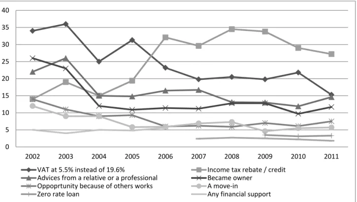
among households, 53 % of them were aware of it in 2005, and more than 80% since 2009, and has been considered by households as the most decisive incentive since 20065. After CIDD’s implementation, other
economic instruments were created. A zero rate loan started in 2009 but has not been used as much as CIDD (around 5% of average recourse rate). An energy‐efficiency certificate (or white certificate) scheme, in which residential energy savings measures were eligible, started in 2006, but this instrument has more to do with the supply side and is nearly unknown among consumers.
Due to its success, CIDD has led to large public expenses: €985 million in 2005, €1.9 billion in 2006, €2.2 billion in 2007, €2.8 billion in 2008, €2.6 billion in 2009, €1.96 billion in 2010 and €1.1 billion in 20116.
In this context, assessing the extent to which free‐ridership may undermine the effectiveness of CIDD became a burning issue. Free‐riding (also called windfalls gains) can be depicted in several ways (Cohen & al. 2012). We define it as the situation in which the subsidized household would have undertaken an energy saving investment even in the absence of the subsidy. The objective of this article is to assess the impact of the CIDD on energy savings investments on both the extensive and intensive margins. The extensive margin corresponds to the number of retrofitting investments that were actually triggered by the CIDD implementation, in other words the CIDD’s effect on the probability to retrofit, whereas the intensive margin measures the adjustment in households’ energy conservation expenditures after the implementation of the CIDD. Those estimations will provide clues to assess the free‐ridership rate, as well as the “economic leverage”, defined as the amount of additional private investment triggered by 1€ of public expense.
We analyze the results of an annual survey conducted for several years before and after 2005 to estimate the impact of the implementation of the CIDD. The “Energy Management” (EM) survey is annually supervised by the French Agency for Environment and Energy Management (ADEME) and carried out by the French market research institute TNS Sofres (TNS Sofres et ADEME 2012). It provides detailed information on the retrofitting decision process, the retrofit options, the households’ and dwellings’ characteristics, and on the subsidization. To insure an homogeneous level of energy performance in the retrofitting measures which modalities can vary with income, retrofitting performance, etc. 5 See Figure 4 in supplementary material for more details. 6 Data from the Public Finances general Directorate (DGFiP).
considered and a sufficient number of observations in order to provide robust statistics7, this study is
focused on insulation measures, which include opaque surfaces insulation (walls, indoor or outdoor insulation, roofs, ceilings, floors) and glazed surfaces insulation (windows, doors, shutters). We use data from 2001 to 2011 and perform a before/after estimation. We conduct preliminary analysis to check the absence of trend and the identification of the CIDD impact.
Our results suggest a significant and positive effect of CIDD on the investment decision on both margins but with a period of latency during the first two years. Estimated CIDD’s effects then progressively increase until 2010, reducing the free‐riding rate, from 79% in 2007 to 43% in 2010, in line with the evolutions in the tax credit rates. Focusing on opaque surfaces insulation measures, CIDD’s effects has only been significant from 2009 onwards, which has to be related to the reform occurring in 2009 including labor cost in the tax credit base for these retrofitting measures. Finally, we find an annual amount of additional private investment generated by 1€ of public expenses going from 1 to 7€.
We first review the implementation of the tax credit in France and the economic literature in section 2. Section 3 describes the data and the model variables. Econometric methods are explained in section 4. Section 5 presents some descriptive statistics and the econometric results. Those are discussed in section 6, before presenting concluding remarks in section 7.
2. Review of the literature and of the French tax credit scheme
2.1. Literature review.
The first references on tax credit dedicated to energy savings investments in the residential sector appear in the economic literature in the context of post oil price shock period. The tax credit implemented in the United States of America (USA) by the Energy Tax Act (ETA) from 1977 to 1986 has been notably extensively studied. This federal tax credit allowed for a 15% reduction of the tax income liability of the amount spent for eligible conservation equipment and could be cumulated with state tax credits. No consensus is found in the literature on the ETA's tax credit incentive effect. Especially, concerns were raised
7
about the ETA's tax credit economic efficiency and potential free‐ridership. Dubin et Henson (1988) hence studied ETA effects on the 1979 tax year, using fiscal data aggregated by Internal Revenue Service (IRS) district and audit class. They assessed the ETA tax credits’ effects on both the probability to declare conservation investment and on the amount of expenditures. They found no significant incentive effects, suggesting that the ETA tax credits had “largely provided windfalls gains to households who would have insulated anyway” (Dubin & Henson 1988). Using micro data from the 1982 Residential Energy Consumption Survey, Walsh (1989) did neither found any significant incentive effect of ETA tax credit on the probability to retrofit. On the other hand, Hassett et Metcalf (1995) found a positive significant incentive effect of ETA tax credit on the likelihood of performing energy‐efficiency improvements, using micro panel data covering 1979/1981 and an alternative definition of the tax credit variable. However, these authors did not assess any free‐ridership rate.
Another wave of tax credit implementations has occurred more recently in the context of global warming awareness, leading to a new range of studies. Using cross‐section data from the 2005 German Residential Consumption Survey (2128 households) in a discrete choice model, Grösche and Vance (2009) estimated a free‐rider share of about 50%, defined as the part of grant beneficiaries for which willingness to pay exceeds costs in the absence of grant. Using a more flexible discrete choice model on the same database, Grösche & al. (2009) assessed the amount of public expenses assigned to free‐riders in function of the level of subsidy, showing that increasing the grant level made free‐ridership decrease. But with a grant representing 50% of the investment cost, they showed that the amount of public expenses diverted by free‐riders was still very high (70%). Alberini & al. (2013) studied the effects of a tax credit similar to CIDD implemented in Italy in 2007 and showed that the free‐ridership was stronger for heating system replacements than for window replacements. They also found that the free‐ridership was “heterogeneous across the territory” but did not estimate the free‐rider share. They actually suggested that the tax credit has led to an increase in the windows’ replacement rate of 37 to 40 percent in the colder regions only. In France, Mauroux (2012) used tax declarations data to analyze the effects of the 2006 exogenous 12% increase of the CIDD tax credit rate for investments in old buildings after a recent housing transfer. Her results suggest the presence of an important free‐ridership effect in the case of a marginal increase of the
tax credit rate. However, she did not investigate the effect of the tax credit introduction.
2.2. The French tax credit scheme
8.
The French tax credit scheme CIDD started in 2005. Tax credit was initially implemented between 2005 and 2009 and then extended until 2015. It could possibly run later on. The purchase of energy efficient durables for the main home9 is eligible for income tax credits, with rates ranging from 15 to 50% of
investment cost. Eligible investments include both energy conservation measures and renewable energy systems. As for conservation, it applies to insulation, for both opaque surfaces and windows/shutter, and to heating system improvements, such as heating regulation systems (mainly including thermostatic valves and programming equipment) and performing systems (low‐temperature and condensation boilers). Renewable energy production refers to wood‐heating appliances, photovoltaic panels, solar heaters and domestic wind turbines. Tax credit subvention is capped at 8 000€ for a 1 person dwelling, 16 000 € for a 2 persons dwelling (with surplus per child) for a 5 consecutive years period. Renewable energy production systems (including heat pumps) are eligible for all types of building, whereas insulation measures are only eligible for building older than 2 years. Tax credit rates are specific to each retrofitting types and are based on energy performance criteria. Table 1 gives details for tax credit rate evolutions. Inside each category, rates have evolved through time and can be specific to certain households’ situations. Evolutions in the tax credit rates, as well as energy performance eligibility criteria, have resulted from a compromise between the aim of targeting the most energy efficient systems, the will of limiting public expenses and the lobbying from the supply side. Heat‐pumps are a good example: air‐air heat‐pumps were only eligible between 2006 and 2008 whereas thermodynamic heat‐pumps for water heating started to be eligible in 2010. As regards specifically opaque surfaces specifically, whereas the tax credit base had only subsidized material cost since 2005, it included labor cost (installation expenditures) in the tax credit 8 This review of the French tax credit scheme is based on information coming from the several Official Tax Bulletin publications (BO n°147 on September 2005, BO n°183 on May 2006, BO n°88 on July 2007, BO n°38 on April 2009, BO n°65 on June 2009, BO n°77 on August 2010, BO n°84 on December 2011) and public reports or publications (Mauroux, Clerc, et Marcus 2010) (Pelletier 2011) (Mauroux 2012).
9
Tax credit had only subsidized owner‐occupiers and tenants but was extended to landlords renting their dwelling in 2009.
base in 200910. Finally, an overall tax credit cut of 10% (called “rabot” in French) occurred in 2011, due to the economic crisis and concerns about public deficit. Table 1. Tax credit rate evolution. 2001/2004 2005 2006‐2007 2008 2009 2010 2011‐2012 Insulation Roof and wall 0% 25% 25%/40%* 25%/40%* 25%/40%* 25% 22% Floor 0% 25% 25%/40%* 25%/40%* 25%/40%* 25% 22% Ceiling 0% 0% 0% 25%/40%* 25%/40%* 25% 22% Window, shutter 0% 25% 25%/40%* 25%/40%* 25%/40%* 15% 13.50% Energy production Heating regulation syst. 0% 25% 25%/40%* 25%/40%* 25%/40%* 25% 22% Low‐temperature boiler 0% 15% 15% 15% 0% 0% 0% Condensing boiler 0% 25% 25%/40%* 25%/40%* 25%/40%* 15% 13.50% Wood heating appliance 0% 40% 50% 50% 40% 25%/40%** 22%/36%** Specific heat‐pump 0% 40% 50% 50% 40% 25%/40% 22%/36% Renewable energy 0% 40% 50% 50% 50% 25%/50%*** 22%/45%***
(*) 25% in the general case, 40% for housing transfer (move‐in date less than 3 years before retrofitting) in old constructions (built before 1977).
(**) 25/22% in the general case, 40/36% in the case of replacement.
(***) 25% for photovoltaic panels, 50% for others (solar heater, domestic wind turbines, ...)
3. Data
3.1. Dataset description
The data used in this paper come from the annual “Energy Management” survey (EM survey) supervised by the French Agency for Environment and Energy Management (ADEME) and conducted by the French market research institute TNS‐Sofres. It provides detailed information on the retrofitting decision process, the retrofit options, the households and dwellings characteristics, and on the subsidies they received. We used data collected from 2001 to 2011. This survey is based on a renewed panel of households, the number of annual observations going from 6148 households in 2005, to 8498 in 2008. Although TNS‐Sofres states that about 25% of the sample is renewed each year, the average turnover rate between two successive years was in reality 49.4%. We therefore analyzed data as cross section to avoid dropping too many observations. Every year, households are asked about their residential energy consumption and the investments they have or not made, in order to improve the energy efficiency of their
10
dwelling. A first questionnaire provides socio‐economic variables, housing information (type of building, heating energy source, building date, etc.), and information about dweller's situation (occupation status, move‐in date). Those who have invested in retrofitting during the last year (7‐12% each year) answer a second questionnaire to provide information on retrofitting types, investment costs, some payment modalities, the economic or non‐economic incentives investors have benefited from (including tax credit), as well as other qualitative information such as their motivation, personal context, satisfaction, etc. In this second questionnaire, each investment is described by 1 to 4 items taken from a retrofitting options list. Retrofitting options include insulation (external insulation of wall, internal insulation of wall, roof, attic, ceiling, windows, shutters), heating system improvement (thermostatic valves, heat cost allocators, ambient thermostat, programming equipment), new heating system (radiator, boiler, wood stove, heat‐ pump, solar heater) or heating system replacement (with information on fuel switching).
3.2. Variables selection
The dependent variables we picked up in the EM survey dataset are: the retrofitting investment
decision and the investment cost. The binary variable “retrofitting investment decision” is equal to one if the
respondent has invested in retrofitting during the past year. This variable allows for the assessment of the CIDD’s effects on the investment decision on the extensive margin. We have restricted our analysis to the retrofitting measures that were: i) homogeneous enough regarding energy performance and CIDD’s eligibility, and ii) frequently found each year and over the period11. This leads us to retain only the opaque
(roofs, indoor walls, outdoor walls, ceilings, floors) and glazed (windows, shutters) surfaces insulation types. The investment cost variable quantifies the expenditures reported for each retrofitting type. It was included as a model dependent variable to assess the CIDD’s effect on the intensive margin.
The explanatory variables were selected based on the abundant literature on households’ investment modeling in residential energy, which provides guidance on the main drivers and barriers to consider (Jakob 2007). The basics of those models consists in calculating the return on retrofitting investment by comparing its initial cost with its future economic savings in a cost benefice analysis, in which
11
technological, socio‐economic and contextual constraints can interact.
In our model, the socio‐demographic variables influencing the investment decision were the
Annual income of the dwelling and the age of the head of the household. The Annual income of the dwelling
determines the households’ financial possibilities and their opportunity cost of time12. This variable can also
reflect the households’ discount rate, included in each profitability calculation. Indeed, several studies showed that the discount rate, in other words the preference for the present, decreases with income (Train 1985). Besides, this variable can reflect the impacts of the overall economic variations on individual situations, notably the potential consequences of the crisis occurring at the end of the period. Given life cycle theory, the age of the head of the household may also reflect the financial and situational constraints of the dwelling. Despite the fact they may influence the investment decision, other survey variables, such as the dwelling size or the socio‐professional category13, were not included in the model, as preliminary
econometric analysis suggested low significance in their effects. In order to capture evolutions in individual preferences about the environment and the economic context, possibly linked to either macroeconomics or social evolutions, we also included data on households’ main concerns. In the EM survey, households are hence asked every year to rank by order of importance their concerns about environmental (e.g. pollution, climate change, renewable energy…) and economical contexts (unemployment). Environmental concern and Economic concern were included as explanatory dummy variables, which equaled one if the household had claimed that pollution, and, respectively, unemployment, were one of their main concerns. To describe the household’s situation in their dwelling, we used the status of occupation (rental or
ownership), which is a key variable to characterize the important barrier linked to the split incentives
between renters and owners. The move‐in‐date was also included as explanatory variable, because the households often retrofit just after moving into a new dwelling.
The building completion date, building type, surface area in m2 and heating energy sources were
used to describe the home characteristics, in order to determine the energy performance of a given retrofitting measure and thus condition the profitability of the investment. The building type variable
12
Since the information collection and the implementation phases of a retrofitting project are time consuming. 13
Households’ awareness of energy efficiency issues or their abilities to undertake retrofitting themselves (requiring time and manual skills) can be correlated with the socio‐professional category.
differentiates between individual houses and collective flats. It also characterizes the potential barriers raised by a collective decision process. The Heating degree days (HDD) and the category of city were used to represent the climatic and spatial characteristics of the dwelling. The regional HDD variable, taken from external data source14, influences the energy performance of a retrofitting investment, as the energy needs
vary according to the outside temperature. The category of city, allows for the differentiation between urban and rural regions, and captures aspects such as storage space availability or supply‐side structure of the residential energy efficiency market.
Finally, we also included explanatory variables characterizing the household’s economic environment, including the presence of CIDD, and other information such as the fact that the dweller is entirely, partially, or not in charge of the expenses and the status of the retrofitter (declared professional or not)15. As for the benefice calculations’ part16, we included the average heating energy price of the current
year (assuming myopic anticipation) as explanatory variable aiming at translating energy savings into economic gains17. The energy prices were determined on the basis of the main energy source declared by each household (electricity, gas, fuel, wood, district heating and a mix between electricity and wood).
14
From statistics made by the French Ministry of Ecology. http://www.statistiques.developpement‐durable.gouv.fr/energie‐ climat/r/statistiques‐regionales.html?tx_ttnews. Heating degree day (HDD) is a measurement based on the gap between outside temperatures and an inside temperature of comfort. The heating requirements for a given structure at a specific location are considered to be directly proportional to the number of HDD. 15 Hiring a professional declared retrofitter is a necessary condition to benefit from the tax credit. 16 Retrofitting prices are assumed to be constant over the period once having taken into account inflation by the INSEE household consumer prices index: http://www.bdm.insee.fr/bdm2/choixTheme.action?request_locale=en&code=20. 17
From statistics made by the French Ministry of Ecology. http://www.statistiques.developpement‐durable.gouv.fr/energie‐ climat/r/industrie‐1.html?tx_ttnews[tt_news]=21083&cHash=fb5b458ff78e44f761db201e5f4a2641. No available data for wood domestic price for 2000,‐2002 and 2004 and for district heating before 2003.
4. Econometric strategy
Different modelling approaches can be found in the tax credit literature. Some consider tax credit as a pure economic incentive. For example, Grösche and Vance (2009) use a discrete choice model in which the tax credit is identified as the subsidized financial amount to be counted down from the investment cost. However, a tax credit based on energy performance criteria can have a two‐fold effect: an “announcement effect” and a “price effect” (Koomey 2002). The price effect simply reflects the fact that the subsidy improves the profitability of the investment. The announcement effect comes from the credibility conferred to certain goods by the regulator. It acts as a label. Indeed, investment decision for residential energy efficiency is a long process, in which tax credit can act through both channels. The maturation period of a renovation project lasts more than 6 months, according to the OPEN18 database, all the more for a projectincluding insulation measures (OPEN 2008). This time period is necessary to gather information on the technologically and economically complex energy efficiency investments. The maturation time of the project varies as a function of the initial knowledge of the households, and other intangible costs such as apprehension faced to the disturbance, uncertainty about future energy prices, the opportunity cost of time, etc. This two‐fold effect prevents us from identifying CIDD to the level of subsidy only, e.g. tax credit rate, as it would only reflect the price effect.
Besides, heterogeneity in tax credit rate mainly depends on retrofitting types. Therefore, tax credit rate determination would be endogeneous to the households’ choice. Moreover, tax credit rates for insulation measures would be too homogeneous over the period to provide a good identification.
We considered that the EM survey variable relative to tax credit awareness was not a good proxy for the announcement effect, as it might be endogeneously biased by inverse causality19 and omitted
variables20. Therefore, taking advantage of the large timespan of the data and following Alberini & al. (2013) we 18 OPEN data come from a survey similar to the “Energy Management” survey, from which our data come from, but provides only 3 years of data after 2005, so it could not be used for our econometric study. 19 Bias due to inverse causality bias occurs if the decision to retrofit also makes households be aware of CIDD. From Open survey, 16 to 17% of investors stated that they had learned of the existence of tax credit after having decided to engage a retrofitting project. 20 Bias due to omitted variables occurs if unobservable factors influence both the probability to invest in energy conservation and the probability to know about tax credit. People's unequal awareness of fiscal incentives can be related to their socioeconomic profile (age, socio‐professional category, income but also the social network e.g. word of mouth), the place where they live, etc. These factors can also impact their investment decision.
have performed a before/after estimation to identify the CIDD effects.
4.1. The “before/after” estimation.
Let
ˆ
BA be the before/after estimator: 1 0 ˆBA CIDDit CIDDit it it Y Y (1) withY
itthe dependent variable, e.g. the retrofitting investment decision or the investment cost, CIDDit 1it
Y
and CIDDit 0
it
Y
the empirical means ofY
itafter and before CIDD’s implementation, respectively. LetCIDD
itbe a dummy variable equal to one after CIDD’s implementation and zero before.
ˆ
BAcaptures the average effect of CIDD’s introduction on the dependent variable. It is identified by the marginal effect ofCIDD
it onit
Y
and is unbiased if all unobserved explanatory variables are constant over time (Crépon et Jacquemet 2010).Therefore, all variables that are relevant in the investment decision and are likely to have evolved during the time period considered have to be included in the model. The eventual presence of trends in these potential time‐varying variables must however be checked in the dataset corresponding to the period before CIDD’s implementation, in order to make sure that these trends are not captured in the CIDD effects.
4.2. Econometrics specification.
We first aimed at determining the amount by which the probability to invest was increased when households benefited from a partial refund of their expenditures. To estimate this CIDD’ effect on energy saving investments on the extensive margin, we used a dichotomous logit model:(
|
)
(
1|
)
(
)
1
it it X it it it it it Xe
E I
X
P I
X
F X
e
, (2)with
P I
(
it
1 |
X
it)
the probability to invest in retrofitting for the household i at time t and F a logistic cumulative distribution function. Given a set of exogenous variablesX
it
(
x
1it,...,
x
kit)
,
is the vector of coefficients to be estimated. The model is estimated by weighted maximum likelihood.We first checked the absence of temporal trend by fitting the following model on dataset collected before CIDD’s implementation: ' '
(
|
,
' )
(
1 |
,
' )
1
it it Tit Xit T X it it it it it ite
E I
T X
P I
T X
e
(3) , withT
itthe trend over the 2001/2004 period andX
'
it
(
x
1it,...,
x
kit)
the exogenous variables on households and dwellings characteristics, as presented in section 3.2, and
the vector of their corresponding coefficients. Then, we fitted the full model over the 2001/2011 period: ' '(
|
,
' )
(
1 |
,
' )
1
it it CIDDit Xit CIDD X it it it it it ite
E I
CIDD X
P I
CIDD X
e
(4) , withCIDD
it the dummy equal to one after CIDD’s implementation and zero before with
its coefficient andX
'
it
(
x
1it,...,
x
kit)
the same other exogenous variables.Contrary to linear model, before/after estimate BA
is not directly derived from
. Indeed, marginal effects of a particularx
ikonP I
(
it
1 |
X
it)
write:(
1 |
)
(1
(
1 |
)) (
1 |
)
it it k it it it it kitP I
X
P I
X
P I
X
x
. (5) In order to estimate BA, we computed marginal effects at the means of the sample using the delta method. For quantitative exogenous variables, marginal effects are the derivative of the predicted probability P Iˆ ( it 1 |Xit) at means of(
X
it i)
1,..,N, i.e. the effect of one unit increase of the explanatory variable on the probability to retrofit. For qualitative variable, each modality of the variable is transformed into dummy and the marginal effect is the effect on the predicted probability to retrofit of being into aparticular modality rather than the modality of reference:
(
1 |
)
ˆ
ˆ
(
1 |
1, )
(
1 |
0, )
it it k k ikP I
X
P I
x
x
P I
x
x
x
. (6)In a second time, we aimed at determining the amount by which the households that invested in energy efficiency adjusted their investment after the implementation of the CIDD. To estimate this CIDD’s effect on energy saving investment on the intensive margin, we fitted a linear model by Ordinary Least Squares (OLS) on the subsample of people who invested in retrofitting:
'
it it it it
Y
CIDD
X
u
, (7),with
Y
itthe total investment costs of each retrofitting measures of household i at time t,1
'
it(
it,...,
kit)
X
x
x
the exogeneous variablesCIDD
it the same as defined in equation (4), andu
itthe residuals. As the households solely report their own expenses, the sample only includes the investments they entirely paid for, in order to avoid the inclusion of shared (with the owner, the co‐owners...) investments costs, that would bias low the equipment real value. Although auto‐produced retrofitting measures are not eligible to CIDD, the sample includes retrofitting measures produced by both professionals and/or the household in order to take into account the potential report of auto‐producers toward professionally produced retrofits. Indeed, the rate and base of the subsidies can make the professional realizations more profitable, especially in the case of opaque surface insulation after the 2009 reform (inclusion of labor costs in the tax credit base), and then change the arbitrage between auto and professional production. In addition to the explanatory variables used in the previous models,1
'
it(
it,...,
kit)
X
x
x
includes dummies for each insulation measure type, since they have different cost levels, the surface area of the dwelling, an Invoice dummy variable equal to one if the household expenses were based on an invoice, and an Auto‐production dummy equal to one if the retrofitting had not been made by a professional. In this model, the before/after estimate BAis directly identified by
.5. Results
5.1. Descriptive statistics
Annual investment rates for both opaque and glazed surfaces insulation measures are presented in Figure 1. Investment rates were relatively steady before 2005 and started to increase after 2005, especially in 2009. This suggests that differentiated effect occurred during two sub‐periods of CIDD’s implementation: Figure 1. Retrofitting rate in % of all households. 2005/2008 and 2009/2011. The difference between the two sub‐periods could reside in the addition of the installation expenditures in the tax credit base in 2009 (cf. econometrics estimations). Figure 2 details investment rates for opaque surfaces insulation. Roof insulation was the most common opaque surface insulation measure over the period, and also the retrofitting work that has increased the most after the CIDD implementation, especially after 2009. Other opaque surfaces insulation measures series do not show any marked trend, except from a slight increasing trend for indoor wall insulation during the CIDD period. Investment rates in retrofit combinations (2 or 3 opaque surfaces insulated in a row) were consistently inferior to unitary insulation investment rates, in spite of the fact they are known to more efficiently improve the energy performance. They remained stable over the study period, except from with a slight increase in the combination of 2 insulated opaque surfaces. 2 2.5 3 3.5 4 4.5 5 5.5 6 6.5 2001 2002 2003 2004 2005 2006 2007 2008 2009 2010 2011 Rate in %Opaque and glazed surfaces insulation measures.
Opaque surfaces insulation measures.
Figure 2. Retrofitting rate in % of all households by opaque surface insulation measures.
Table 2 gives the results of a Pearson's chi‐squared test statistic testing the equality between the investment rates during the pre (2001‐2004) and post (2005‐2011) CIDD periods for opaque surfaces insulation and window insulation measures.
Table 2. Pearson's chi‐squared test statistic.
Investment rate (in %)
Test
power* Statistic P Value**
2001/2004 2005/2011 Insulation measures: All opaque surface 2.57 3.29 11410 42.59 0.00 Internal wall 0.54 0.67 73974 6.42 0.01 External wall 0.22 0.23 2733525 0.13 0.72 Roof 0.76 1.25 8526 54.95 0.00 Ceiling 0.26 0.25 3641188 0.1 0.76 Floor 0.18 0.15 419717 1.06 0.30 2 opaque surfaces 0.52 0.63 98491 4.81 0.03 3 opaque surfaces 0.08 0.1 1354310 0.25 0.62 Window insulation 3.46 3.92 36717 13.42 0.00 Total sample size 37380 67558 The null hypothesis H0 is the equality between the two investment rates over 2001/2004 and over 2005/2011. * The power of the test gives the minimum number of observations required in each group to provide robust test statistics given a Type I error probability fixed at 5%. ** H0 is rejected when the p‐value is less than the predetermined significance level (5%). 0 0.2 0.4 0.6 0.8 1 1.2 1.4 1.6 1.8 2001 2002 2003 2004 2005 2006 2007 2008 2009 2010 2011 Rate in %
Internal wall External wall Roof Ceiling
The equality of the detailed opaque surfaces (except for roofs) investment rates before and after the CIDD implementation could not be tested, due to their small sample size and low power value. We consequently pooled all opaque surface insulation measures in one category to ensure the test good statistical power. The equality of the detailed opaque surfaces investment rates (null hypothesis) is then rejected for both opaque surfaces insulation and windows insulation.
The average annual investment cost in opaque surfaces insulation, including material and labor costs, for households having entirely paid the costs, are presented in Figure 3The average investment in opaque surfaces insulation has remained stable, around 1500€ 2009, until 2007. It then increased above 2000€ 2009 during the 2009‐2011 period. Roof insulation is structurally more expensive than indoor wall insulation. As for the retrofitting rate inFigure 1, a slight decrease appeared in the 2011 indoor wall insulation investments. Average investment costs in other detailed opaque surfaces are not shown inFigure 3, due to their high annual variability. Average investments in glazed surfaces insulation21 steadily increased
from 2005 (3873€ 2009) to 2010 (4482€ 2009), without any shock in 2009 contrary to opaque surfaces insulation, but with a slight new decrease in 2011 (4323€ 2009). However, the absence of trend before 2005 is less clear and will have to be check in the econometrics. Figure 3. Average investment cost per retrofitted dwelling for retrofitting measures entirely paid by the households (in € 2009, taken into account inflation by the Consumer Index Price). 21 See Figure 7in supplementary material for more details. 500 1000 1500 2000 2500 3000 2002 2003 2004 2005 2006 2007 2008 2009 2010 2011 in euros 2009
Table 3 presents the summary statistics of the households’ socio‐ economic variables and dwellings characteristics computed on different subsamples to better assess the CIDD effects on energy efficiency investments. Table 3. Statistics on socio economic variables and dwellings characteristics. 2000/2011 2000/2004 2005/2011 CIDD aware* Retrofitting* CIDD benefice* Percentage in columns Annual income of the dwelling <18500€ 35.88 39.86 33.69 28.37 24.3 21.42 18500 /36 300€ 44.97 45.32 44.77 47.15 50.01 51.58 >36 300€ 19.16 14.82 21.54 24.48 25.69 27 Head of household's age 34 years old 2.52 2.66 2.44 2.39 1.11 0.2 35‐54 years old 45.1 46.56 43.82 45.6 43.78 36.8 > 55 years old 52.38 50.78 53.74 52.01 55.11 63 Environmental concern 52.48 54.83 51.5 53.98 51.36 51.08 Economic concern 61.81 58.19 63.32 61.97 62.77 62.08 Move in date < 3 years 19.2 19.78 18.6 19.48 21.53 16.77 3 / 10 years 32.09 31.88 32.57 33.7 29.92 25.86 > 10 years 48.71 48.34 48.83 46.82 48.55 57.36 Status of occupation renter 32.83 32.63 32.8 28.07 7.19 1.44 owner 63.94 64.12 63.96 68.85 90.29 96.81 other 3.23 3.25 3.24 3.09 2.52 1.75 Building completion date <=1948 27.73 28.49 26.85 26.95 35.69 29.7 1949/1974 32.99 33.73 32.34 31.36 35.68 40.63 1975/1981 13.41 14.05 13.15 13.27 14.25 17.4 1982/1988 8.84 9.44 8.44 8.66 7.47 7.94 1989/last year 16.22 13.53 18.37 18.86 6.39 4.07 current year 0.8 0.75 0.84 0.9 0.51 0.27 Building type individual house 53.34 51.05 55.91 59.72 78.84 76.06 collective flat 46.51 48.77 43.95 40.14 21.03 23.87 other 0.15 0.18 0.13 0.14 0.12 0.07 Category of city Parisian agglomeration 15.48 15.88 15.19 14.79 9.84 11.55 >100.000 inhabitants 29.2 29.53 29 28.01 23.29 24.86 20.000/100.000 inhabitants 13.2 13.18 13.18 12.88 12.94 14.63 2.000/20.000 inhabitants 17.57 17.45 17.7 17.8 19.79 19.22 Rurals 24.55 23.95 24.94 26.53 34.14 29.74 Means HDD (heating degree days) 2023.20 2025.41 2021.67 2021.29 2047.90 2041.39 Heating energy price 0.0802 0.0695 0.0866 0.0849 0.0817 0.0791 * CIDD aware sub‐sample: households aware of CIDD after 2005; Retrofitting sub‐sample : households having invested in retrofitting after 2005; Benefice CIDD sub‐sample : households having retrofitted and intended to benefit from CIDD after CIDD
19
These are: i) the full sample 2000-2011 dataset, ii) the pre-CIDD subsample (2000-2005), iii) the post-CIDD subsample (2005-2011), iv) the CIDD-aware dwellers subsample, v) the dwellers having invested in opaque or glazed surfaces insulation after 2005 subsample, and vi) the dwellers who invested in opaque surface insulation and intended to benefit from CIDD subsample.
Lower income households are under-represented among investors and CIDD beneficiaries, as the lowest income bracket represents 33.7% of the post-CIDD sub-sample, 24.3% of the households having invested in insulation and 21.4% of the CIDD beneficiaries. Older households are over represented among CIDD beneficiaries as they represent 63% of this subsample whereas they represent 53.7% of the post-CIDD sample and 55.1% of the households having invested. In the same way, owners dominates the CIDD beneficiaries as they are 96.8% of this subsample whereas they represent 64% of the 2005-2011 subsample and 90.3% the households having invested. Households living in rural areas invested more in energy efficiency than urbans but benefited less from CIDD: they are 24.9%, 34.1% and 29.7% of the post-CIDD datasets, the investors and the CIDD beneficiaries, respectively. This might be due to the fact that rurals have more capacities to retrofit by auto-production than urbans, auto-production being the main cause of CIDD ineligibility. Environmental concern was higher between 2001 and 2004 than during the 2005-2011 period (54.8% of the household top priority was environment over 2001/2004, 51.5% over 2005/2011). Conversely, the economic concern increased during the whole 2001-2011 period (unemployment was the top priority of 58.2 and 63.3% of the households during the 2001-2004 and 2005-2011 periods, respectively). Annual national surveys in fact indicates that the environmental concern of French households started to decline after 2008, while employment was becoming the main concern, probably as a side-effect of the economic crisis.
5.2 Econometrics
We first estimate the CIDD effect on energy saving investments on the extensive margin, that is to say by how much is increased the probability to invest when households benefit from a partial refund of their expenditures. Table 4 presents the results of the logit models fitted on the pre-CIDD sub-sample on
one hand, and on the whole dataset (2001‐2011) on the other hand. The binary dependent variable is the decision to invest or not in retrofitting.
The temporal trend had no significant effect on the probability to invest in opaque and glazed surfaces insulation measures or opaque surfaces insulation in the logit model fitted on the pre‐CIDD sub‐ sample. This allows for the implementation of the before/after estimation. Moreover, the estimated marginal effects of most of the covariates had the same level of significance and the same magnitude in the pre‐CIDD and in the full dataset models. This was not the case for variables aggregated over long periods, such as HDD and Heating Energy price, likely due to the large differences in their degrees of freedom between the pre‐CIDD and the full sample.
The results of the logit model fit on the whole dataset reveal determinants that have a highly significant positive effect (at the 1% confidence level) on the investment decision. The household income positively impacts the retrofit decision but the coefficient of the head of household's age is no significant. Households living in old building and/or in individual houses are hence more prone to invest than those living in collective flats. The owner‐occupiers, the households having recently moved in also invest significantly more in energy efficiency. Environmental and economic concerns respectively have a positive and negative effects on the investment decision at the 5% confidence level (only in case of opaque surface insulation for the economic concern). Regarding geographic patterns, households living outside Paris, in small cities or in rural areas, invest more in energy efficiency. The heating degree days (HDD) regional average is no significant but positively impacts the retrofit decision at the 1% confidence level in regressions omitting individual preferences (as individual preferences are correlated to regional HDD averages). Finally, the heating energy price has no significant effect on the investments in opaque and glazed surfaces insulation but has a positive and significant effect (at the 5% confidence level) focusing on opaque surface insulation measures. This suggests that the perspective of energy savings significantly triggers investments in opaque surfaces insulation only.
The annual CIDD effect is presented in columns (2) and (4) of Table 4.After a two‐year latency period (2005‐2007), the CIDD starts to have a significant positive effect on opaque and glazed surfaces insulation investments in 2007. This positive effect increased after 2009 and decreased in 2011. Looking at
opaque surfaces insulation only, CIDD has no effect (at the 1% confidence level) on investments before 2009, except in 2007. This corroborates the descriptive statistics Table 4. Logit’s estimated marginal effects at means on the probability to invest. Opaque & glazed surfaces Opaque surfaces only 2001/2004 2001/2011 2001/2004 2001/2011 (1) (2) (3) (4) (5) Variables Trend 0 ‐0.001 Environmental preferences 0.006** 0.004*** 0.003** 0.002** 0.002* Economic concern ‐0.003 0 ‐0.003* ‐0.002** ‐0.002** CIDD dummy (1st year 2005) 0.002 0.001 CIDD dummy (2nd year 2006) ‐0.003 0 CIDD dummy (3rd year 2007) 0.007*** 0.004*** CIDD dummy (4th year 2008) 0.008*** 0.003* CIDD dummy (5th year 2009) 0.021*** 0.008*** CIDD dummy (6th year 2010) 0.024*** 0.01*** CIDD dummy (7th year 2011) 0.011*** 0.006*** CIDD dummy (period 2005/2008) 0.002* CIDD dummy (period 2009/2011) 0.008*** HDD ‐0.004 0.002 ‐0.007*** 0.002 0.002 Heating energy price 0.018 ‐0.029 0.017 0.022** 0.021** Annual income of the dwelling (ref : <18500 euros) 18500 /36 300 euros 0.006* 0.009*** 0.002 0.002* 0.002* >36 300 euros 0.01** 0.009*** 0.004* 0.002** 0.003** Move in date (ref : < 3 years) 3 / 10 years ‐0.028*** ‐0.041*** ‐0.01*** ‐0.02*** ‐0.02*** > 10 years ‐0.04*** ‐0.054*** ‐0.015*** ‐0.028*** ‐0.028*** Building completion date (ref : < 1974) 1975/1988 ‐0.026*** ‐0.015*** ‐0.007*** ‐0.008*** ‐0.008*** 1989/last year ‐0.055*** ‐0.051*** ‐0.016*** ‐0.018*** ‐0.018*** Status of occupation (ref : renter) owner 0.043*** 0.061*** 0.011*** 0.02*** 0.02*** other 0.014* 0.023*** 0.001 0.006*** 0.006*** Building type (ref : individual house) Collective flat ‐0.032*** ‐0.028*** ‐0.023*** ‐0.021*** ‐0.021*** Head of household's age (ref : 34 years old) 35‐54 years old 0.017* 0.003 0.007 0.004 0.004 > 55 years old 0.006 0.001 ‐0.001 0.001 0.001 Category of city (ref : Parisian agglomeration) > 20.000 inhabitants 0.001 0.003 0.001 0.002* 0.002* <20.000 inhabitants / rural areas 0.002 0.009*** 0.003 0.007*** 0.007*** Log likelihood ‐3954.3987 ‐15811.4 ‐1958.1918 ‐8350.5 ‐8357.7 Sample size 13080 53126 13080 53126 53126 * significant at 10% level, ** significant at 5% level, *** significant at 1% level. Standard errors are not reported. Column 1: logit’s estimated marginal effects at means on the pre‐CIDD sub‐sample (2001/2004) including all insulation measures. Column 2: logit’s estimated marginal effects at means on the whole dataset (2001‐2011) including all insulation measures. Column 3: logit’s estimated marginal effects at means on the pre‐CIDD sub‐sample (2001/2004) includ. only opaque surfaces insulation. Columns 4‐5 : logit’s estimated marginal effects at means on the whole dataset (2001‐2011) includ. only opaque surfaces insulation.
results, which suggested that the CIDD have had differentiated effects in the 2005‐2008 period on one hand, and in the 2009‐2011 period on the other hand. The CIDD effects on the probability to invest in energy efficiency during these two periods was tested by including a dummy variable coding for the two periods in the logit model. Results presented in column (5) of Table 4reveal that the CIDD effect was significantly positive during both periods, but with a 10 fold higher confidence level during the 2009‐2011 period (10% vs. 1%). Moreover, a Wald test shows that the CIDD marginal effects are significantly different between the two periods, the CIDD effect being four times higher during the 2nd period (0.2 vs. 0.8%).
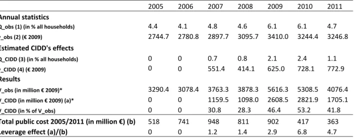
We then derive from those estimations the annual rates of free‐ridership for glazed and opaque insulation investments, after CIDD implementation (Table 5). We remind that free‐ridership is defined as the situation in which the subsidized household would have undertaken the energy saving investment even in the absence of the subsidy. Free‐riding rate equals one minus the rate of additional investors due to CIDD among CIDD beneficiaries. This latter is calculated as the ratio between the additional investment rate due to CIDD, which corresponds to estimated marginal effects, and the rate of people benefiting from the tax credit. Annual free‐ridership rates have globally decreased over the period, dropping from 100% in 2005‐ 2006, when CIDD had no effect on investment decisions, to 79% in 2007, and a 43% minimum in 2010, and finally increasing to 61% in 2011. Table 5. Free‐ridership estimation All retrofit incl. Insulation (opaque and glazed surfaces) 2005 2006 2007 2008 2009 2010 2011 Observed retrofitting rate* 4.44 4.1 4.81 4.64 6.1 6.06 4.65 Observed CIDD recourse rate** 58.51 62.24 69.65 70.55 69.44 70.2 61.59 CIDD beneficiaries (a)* 2.6 2.55 3.35 3.27 4.24 4.25 2.86 Estimated marginal effect of CIDD (b)* 0 0 0.7 0.8 2.1 2.4 1.1 Additional retrofitting due to CIDD*** 0 0 14.55 17.24 34.43 39.6 23.66 Free‐riding rate (1‐ (b)/(a))*** 100 100 79.1 75.54 50.47 43.53 61.54 (*) in % all households in the sample. (**) in % households who have invested in corresponding retrofitting. (***) in % of households who benefit from CIDD for the corresponding retrofitting.
23
We now estimate the CIDD effect on energy saving investments on the intensive margin, i.e. the amount by which the households adjusted their investment after the CIDD implementation. The dependent variable is the total investment cost as explained in section 4.2. Year 2001 data were not included in the analysis, as the investment costs were expressed in French Franc. Table 6 presents the OLS’ estimates obtained with the pre-model fitted on the pre-CIDD sub-sample and with the model fitted on the 2002-2011 sample. No significant temporal trend was found in the model fitted on the pre-CIDD sub-sample for opaque and glazed insulation measures (column 1), neither in models fitted on subsamples comprising opaque and glazed surfaces insulation measures separately22. The estimation coefficients of the retrofit
measures in the model fitted on the 2002-2011 period reveal that the households characteristics effects are less significant in this model than in the extensive margin model. Households having moved recently in their dwelling invest significantly more (except in the case of opaque surfaces insulation only). However, the status of occupation has no significant effect, likely due to the small number of retrofitting observations realized by renters, and the income effect is nearly no significant.
Investing in opaque surfaces insulation in a recent building increases the cost, which is not the case for glazed surface insulation. Similarly, retrofitting an individual house rather than a collective flat increases the investment cost for opaque surfaces insulation but not for glazed surface insulation. The Heating Degree Days variable has a significantly positive effect only for opaque surfaces insulation. The dwelling surface area has a slight positive effect on investment cost, only significant for glazed surface insulation. Heating energy price has a positive but insignificant effect on opaque surface insulation costs and a significantly negative effect on glazed surface insulation costs. This late effect is likely due to structural price differences between energy sources and to correlations between investment costs and energy sources. Indeed, dwellings heated by electricity were mainly built after the first thermal regulations, concerning especially the windows energy efficiency, which decreased the retrofitting need for the electricity-heated dwellings. As electricity prices were much higher than prices of other energy sources, it leads to this apparent inverse relationship between energy prices and investment cost in windows insulation. The same energy source/dwelling building date combination is likely to explain the counter-intuitive positive regression
22