Airline Revenue Management: Sell-up and Forecasting Algorithms by
Thomas 0. Gorin
Ing6nieur des Arts et Manufacture (ECP 1999)
Submitted to the Department of Aeronautics and Astronautics and Center for Transportation Studies
in Partial Fulfillment of the Requirement for the Degree of Master of Science in Transportation
at the
Massachusetts Institute of Technology June 2000
@ 2000 Massachusetts Institute of Technology All rights reserved
Signature of A uthor...
Center for Transportation Studies Department of Aeronautics and Astronautics May 5, 2000 C ertified by... . ... ...
Peter Paul Belobaba Principal Research Scientist Department of Aeronautics and Astronautics Thesis Supervisor Accepted by... ...
Nesbitt W. Hagood
MASSACHUSETTS INSTITUTE Chairman, Graduate Student Program OF TECHNOLOGY Department of Aeronautics and Astronautics
SEP 0 7
2000
Airline Revenue Management: Sell-up and Forecasting Algorithms by
Thomas 0. Gorin
Submitted to the Department of Aeronautics and Astronautics and Center for Transportation Studies
on May 5, 2000 in Partial Fulfillment of the Requirement for the Degree of Master of Science in Transportation
ABSTRACT
Recent technological improvements have allowed airlines to implement sophisticated Revenue Management systems in order to maximize revenues. Computational capabilities make it possible to perform network-based analysis of supply and demand and therefore to increase the gains achieved with the help of "0-D control" Revenue Management algorithms. However, the more commonly used and cheaper flight leg-based algorithms have not yet been used to the best of their potential and can still benefit from better modeling of passenger behavior.
Our first purpose in this thesis is therefore to evaluate the benefits of incorporating sell-up models into current leg-based airline Revenue Management algorithms. Another question we would like to try and address is whether it would be possible to improve the leg-based models to reach revenue gains comparable to those of O-D control algorithms. To try and achieve this goal, we improve the modeling in our leg-based Revenue Management algorithms by accounting for the possibility of sell-up, that is the probability that a passenger will accept a more expensive ticket than originally desired if seats are not available at the lower fare. In addition, previous research has shown that there are revenue gains to be achieved through better forecasting, therefore, we also evaluate the use of better forecasting methods and quantify their revenue impact. In particular, we focus our efforts on understanding the impact of the unconstraining models on revenue gains by using various detruncation methods and comparing their effect.
Thesis Advisor: Dr. Peter Paul Belobaba
Acknowledgments
First of all, I would like to thank my thesis and research advisor Dr. Peter Belobaba for all his help. He provided me with great support and helped me understand all the aspects of Revenue Management that I only thought I understood. Moreover, without his help, I could never have caught all the mistakes I made in this thesis.
I would also like to thank all the PODS Consortium team (Continental Airlines,
KLM, Lufthansa, Northwest Airlines, SAS and Swissair) for their guidance in the research directions and their input and comments on the results. It was always quite
surprising to see all the questions that arose from the presentation of my results:
Most of those questions had never crossed my mind and were a great help in stepping away from the academic perspective to try and understand Revenue Management and Sell-up from a "real world" point of view.
In particular, I especially thank Craig Hopperstad for his enormous help in understanding the models and the subtleties of PODS. Without the simulator and Craig's patience in explaining how to use PODS, this thesis would not have existed.
In addition, it was great working with an amazing team of students at MIT in the International Center for Air Transportation. In particular, Torsten Busacker, Anne Dunning, Alex Lee, Seonah Lee, and Trin Mitra who helped me understand PODS
and/or supported me.
Finally, last but certainly not least, I thank my family for helping me make it to MIT and supporting me every day.
TABLE OF CONTENTS
TABLE OF CONTENTS 7 LIST OF FIGURES 10 LIST OF TABLES 12 INTRODUCTION 13 Revenue Management 13 Forecasting 15 Sell-up 16Goal of the Thesis 17
Structure of the Thesis 18
PART I: THEORY 21
Chapter 1: Pods And Revenue Management 23
1.1 PODS 23
1.1.1 The model 24
1.1.2 Inputs 27
1.1.2.a System Level Input Parameters 28
1.1.2.b Airline Input Parameters 28
1.1.2.c Market Level Parameters 28
1.1.3 Outputs 30
1.1.4 Network 6B 31
1.2 Revenue Management Methods 32
1.2.1 Fare Class Revenue Management Algorithms 33
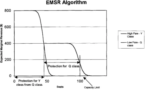
1.2.1 .a Expected Marginal Seat Revenue (EMSR) 33
1.2.2 Origin-Destination Algorithms 36
1.2.2.a Greedy Virtual Nesting (GVN) 36
1.2.2.b Displacement Adjusted Virtual Nesting (DAVN) 37
1.2.2.c Deterministic LP Network Bid Price (Netbid) 38
1.2.2.d Heuristic Bid Price (HBP) 39
1.2.2.e Prorated Bid Price (ProBP) 41
1.3 Summary 42
Chapter 2: Detruncation and Forecasting 45
2.1 Detruncation Methods 45
2.1.1 Booking Curve Detruncation 46
2.1.1 .a Underlying Assumption 46
2.1.1.b The Algorithm 46
2.1.2 Projection Detruncation 47
2.1.2.a Underlying Assumptions 47
2.1.2.b The Algorithm 47
2.1.2.c An Example: AGIFORS 1987 48
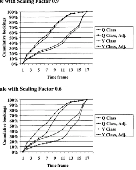
2.1.3 Adjusted Booking Curve 49
2.1.3.a Variation of the Booking Curve Detruncation Method 49
2.1.3.b The correction 50
2.1.3.c Best Scaling Factor 51
2.1.4 Summary 52
2.2 Forecasting: Two Methods 52
2.2.1 Pick-up forecasting 52
2.2.1.a Important Note 55
2.2.2 Regression Forecasting 55
2.3 Objective of Detruncation and Forecasting 56
Chapter 3: Sell-up 57
3.1 Understanding the Mechanisms Involved 57
3.1.1 Passenger Behavior: Leisure vs. Business 58
3.1.2 Maximum Willingness-to-Pay 60
3.2 Bohutinsky's Study 60
3.3 The Belobaba-Weatherford Heuristic 61
3.4 Another Sell-up Algorithm: Brumelle et al. 62
3.5 Objectives of Sell-up 63
PART II: SIMULATION AND RESULTS 65
Base Case 65
Specifications of Our Base Case 66
Chapter 4: Sell-up and Detruncation in a Fare Class Yield Management (FCYM) Environment 67
4.1 Booking Curve Detruncation 67
4.1.1 Airline A Only Accounts for Sell-up 67
4.1.1.a Results 68
4.1.1 .b Conclusion 71
4.1.2 Understanding What Happens 71
4.1.2.a The Heuristic 71
4.1.2.b Loads 72
4.1.2.c Summary 75
4.1.3 Both Airlines Account for Sell-up 76
4.1.3.a Results 76
4.1.3.b Explaining the Results 78
4.1.4 Conclusion 81
4.2 Projection Detruncation 82
4.2.1 Preliminary Results 82
4.2.1.a Only Airline A Accounts for Sell-up 82
4.2.1.b Both Airlines Account for Sell-up 84
4.2.1.c Summary 87
4.2.2 Best t Value and Related Revenues 87
4.2.2.a Decreasing the Protection through the Detruncation Method 88
4.2.2.b Only Airline A Accounts for Sell-up 88
4.2.2.c Both Airlines Account for Sell-up 91
4.2.3 Conclusion 91
4.3 Adjusted Booking Curve 92
4.3.1 Only Airline A Accounts for Sell-up 92
4.3.1.a Constant Sell-up Rates 92
4.3.1.b Differential Sell-up Rates 94
4.3.2 Both Airlines Account for Sell-up 95
4.3.3 Conclusion 96
Chapter 5: Sell-up in a Virtual Bucket Environment 97
5.1 Booking Curve Detruncation 98
5.1.1 GVN vs. EMSRb 98
5.11.a Only Airline A Accounts for Sell-up 98
5.1.1 .b Conclusion 106
5.1.2 Both Airlines Account for Sell-up 106
5.1.2.a Revenues 107
5.1.2.b Loads 108
5.1.3 Conclusion 109
5.2 GVN vs. GVN 109
5.2.1 Only Airline A Accounts for Sell-up 110
5.2.2 Both Airlines Account for Sell-up 113
5.2.3 Summary 115
5.3 Projection Detruncation 116
5.3.1 GVN with Projection Detruncation vs. Base Case EMSRb 116
5.3.1.a Revenues 117
5.3.1.b Loads 118
5.3.2 Effect of the Competitor's Revenue Management Method 119
5.3.2.a Simulations 119
5.3.3 Summary 123
5.4 Conclusion: Sell-up vs. Detruncation -Present Findings 124
Chapter 6: Comparison with Other O-D Methods -Validation of our Results in a Larger Network 127
6.1 Comparison with Other O-D Methods 127
6.1.1 Previous Results 128
6.1.2 Comparison with our Results 129
6.1.2.a Comparison with Earlier Results 129
6.1.2.b Effect of Competitor Using Sell-up on O-D Methods 130
6.1.3 Conclusion 131
6.2 Validation of Previous Results in a more Complex Network 132
6.2.1 Network C 132
6.2.2 Sell-up Results in Network C 134
6.2.3 Influence of Network Size on EMSRb and GVN 134
6.2.4 Comparison with other O-D Methods 136
6.2.5 Conclusion 137
6.3 Observed Sell-up Rates (OSR) 137
6.3.1 Computing the Observed Sell-up Rate 138
6.3.1.a Example 139
6.3.1.b Results 139
6.3.2 Observed Sell-up Rates as a Function of the Demand Factor 140
6.3.3 Influence of Accounting for Sell-up on Observed Sell-up Rates 141
6.3.4 Summary 141
6.4 Conclusion 142
CONCLUSION 143
Summary of Findings 143
Future Research Directions 145
Estimating the Observed Sell-up Rates 146
Incorporating Sell-up Models in other O-D Methods 146
LIST OF FIGURES
F igure 1: P O D S A rchitecture...24
F igure 2 : P O D S F low C hart...26
F igure 3 : N etw ork 6B ... 32
Figure 4: E M SR value of each seat ... 35
F igure 5 : N etbid B id P rices ... 39
F igure 6 : H B P B id P rices ... 40
F igure 7 : P roB P L ogic ... 42
F igure 8: Projection D etruncation ... 48
Figure 9: Pbscale w ith Scaling Factor 0.9 ... 51
Figure 10: Pbscale w ith Scaling Factor 0.6 ... 51
Figure 11: Booking Curves by Passenger Type... 59
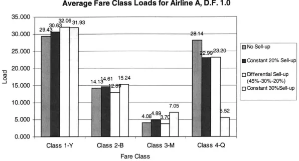
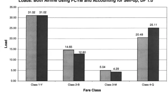
Figure 12: Fare Class Loads as a Function of Input Sell-up Rate, DF 1.0... 73
Figure 13: Average Fare Class Loads for Airline B, DF 1.0 ... 74
Figure 14: A verage Fare Class Loads, DF 1.0... 79
Figure 15: Loads for Airline A as a Function of Competitive Response, DF 1.0... 80
Figure 16: Revenue Gains as a Function of Detruncation and Sell-up, DF 1.0 ... 83
Figure 17: Loads for both airlines with differential sell-up rates and demand factor 1.0 ... 86
Figure 18: Loads for both airlines at differential sell-up rates and demand factor 1.2 ... 87
Figure 19: Percentage Revenue Gains for Airline A as a Function of the t Value and the Demand Factor, Airline A with Differential Sell-up Rates Assumed, Airline B without Sell-up ... 89
Figure 20: Comparison in Loads for Airline A when it Alternatively Uses Projection Detruncation or not, Combined with Sell-up; Airline B Uses Booking Curve Detruncation without Sell-up, DF 1.0 ... 90
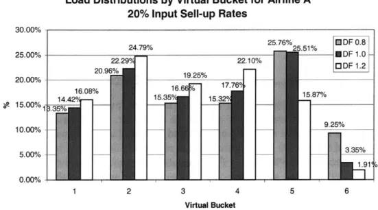
Figure 21: Percentage Revenue Gains as a Function of Assumed Sell-up Rate and Scaling Factor, DF 1.0 93 Figure 22: Load Distributions by Virtual Bucket for Airline A at a Constant Input sell-up Rate of 20% per V irtu al B u ck et... 10 0 Figure 23: Loads by Virtual Bucket at Demand Factor 1.0 and 20% Input sell-up Rate... 101
Figure 24: Passenger Distribution by Virtual Bucket as a function of the Input sell-up Rate, DF 0.8 ... 102
Figure 25: Virtual Bucket Loads at Demand Factor 0.8, as a Function of the Input sell-up Rate ... 102
Figure 26: Comparison between Gains from GVN with and without Sell-up when the Competitor Does Not A ccount for S ell-up ... 104
Figure 27: Loads for Airline A as a Function of the Input Sell-up Rate, DF 1.0... 105
Figure 28: Loads by Virtual Bucket, Airline A with Differential Sell-up Assumed, Airline B w/o Sell-up, D F 1 .0 ... 10 6 Figure 29: Loads by Virtual Bucket, Demand Factor 1.0, Both Airlines Account for Sell-up... 108
Figure 30: Loads by Virtual Bucket for Airline A, depending on the Assumed Sell-up Rate... 109
Figure 31: Load Distribution by Virtual Bucket for Airline A, Depending on the Assumed Sell-up Rate, DF 1 .0 ... 1 12 Figure 32: Loads by Virtual Bucket, GVN with Sell-up vs. GVN w/o Sell-up, DF 1.0, Differential Sell-up R ates A ssu m ed ... 113
Figure 33: Loads by Virtual Buckets as a Function of Input Sell-up Rates, DF 1.0, GVN vs. GVN... 115
Figure 34: Summary of Booking Curve Detruncation Results at Demand Factor 1.0... 116
Figure 35: Airline A Revenue Gains as a Function of T, GVN with Differential Sell-up Assumed vs. E M S R b w /o S ell-up ... 117
Figure 36: Loads by Virtual Bucket, GVN with Differential Sell-up Rates Assumed and Projection Detruncation vs. EMSRb w/o Sell-up and Booking Curve Detruncation, DF 1.0 ... 118
Figure 37: Summary of Revenue Gains for all Cases as a Function of t, DF 1.0... 120
Figure 38: Revenue Gains for Both Airlines in all Four Cases, DF 1.0 ... 121
Figure 39: Revenue Gains as a Function of the Competitive Situation, DF 1.2... 123
Figure 40: Impact of Sell-up Models and Projection Detruncation at Demand Factor 1.0... 124
Figure 42: Revenue Gains as a Function of the Competitive Situation, DF 1.0 ... 129
Figure 43: Revenue Gains for Airline A when Competitor Accounts for Sell-up, DF 1.0 ... 131
Figure 44: N etw ork C G eographical Layout ... 133
Figure 45: Network C Revenue Gains over Base Case (EMSRb vs. EMSRb)... 133
Figure 46: Comparison between Network 6B and Network C Revenues, EMSRb and GVN, DF 1.0... 135
Figure 47: Revenue Gains for all O-D M ethods, DF 1.0... 136
LIST OF TABLES
Table 1: Major Input Parameters in PODS (See Zickus)... 27
T ab le 2 : O -D F ares ... 2 9 T ab le 3 : F en ce s ... 3 0 Table 4: An Example of Virtual Bucketing ... 37
Table 5: M apping the Fares w ith D A V N ... 38
Table 6: Summary of Revenue Management Algorithms Specifications ... 43
Table 7: Application of Projection Detruncation... 48
T able 8: B ookings are biased high... 50
Table 9: H istorical B ookings on H and ... 53
T ab le 10 : P ick -u p ... 5 3 Table 11: Average Pick-up and Standard Deviation... 54
Table 12: Base Case Results at all Tested Demand Factors ... 66
Table 13: Revenue Gains as a Function of Constant Sell-up Rate and Demand Factor ... 68
T able 14: D ifferential Sell-up R ates ... 70
Table 15: Revenue Gains as a Function of Differential Sell-up Rates and Demand Factor ... 70
Table 16: Influence of Sell-up Heuristic on Protections... 72
Table 17: Average Leg Load Factors, D.F. 1.0 ... 74
Table 18: Revenue Gains as a Function of (Constant) Input Sell-up Rate and Demand Factor ... 77
Table 19: Revenue Gains as a Function of (Differential) Input Sell-up Rate and Demand Factor... 78
Table 20: Average Leg Load Factors, DF 1.0 ... 80
Table 21: Comparison in Average Leg Load Factors, DF 1.0... 81
Table 22: Summary of Revenue Gains with Projection Detruncation, T=0. 15 ... 84
Table 23: Percentage Revenue Gains When Both Airlines Account for Sell-up and A Only Uses Projection D etruncation (T=0 .15) ... 85
Table 24: Percentage Revenue Gains for Airline A when both Airlines are Accounting for Sell-up with Differential Sell-up Rates Assumed, and only Airline A is Using Projection Detruncation... 91
Table 25: Percentage Revenue Gains as a Function of Demand Factor and Pbscale Factor, 20% Sell-up R ate p er F are C lass ... 9 3 Table 26: Percentage Revenue Gains as a Function of Demand Factor and Pbsacle Parameter at Various A ssum ed S ell-up R ates ... 94
Table 27: Percentage Revenue Gains when Both Airlines Account for Sell-up... 95
Table 28: Revenue Gains as a Function of Demand Factor and Input Sell-up Rate... 99
Table 29: Revenue Gains as a Function of Differential Input Sell-up Rate, DF 1.0... 104
Table 30: Percentage Revenue Gains as a Function of Demand Factor, Competitive Situation and Input S ell-u p R ates ... 10 7 Table 31: Percentage Revenue Gains for Airline A as a Function of the Demand Factor and Input Sell-up R ates, G V N w ith Sell-up vs G V N ... 111
Table 32: Percentage Gains as Function of Demand Factor and Input Sell-up Rates, GVN vs. GVN... 114
Table 33: PODS output -Actual Choice Given First Choice Percentages ... 139
Table 34: Observed Sell-up Rates for Airline A, by Fare Class ... 139
Table 35: Observed Sell-up Rates as a Function of Demand Factor, EMSRb vs. EMSRb ... 140
INTRODUCTION
In this thesis, our goal is to evaluate the revenue benefits that can be achieved by an airline if it improves its models of passenger behavior. In the recent past, airlines have been looking for ways to increase their revenues. In particular, airlines started segmenting demand through differential pricing, that is, recognizing the fact that there are different types of passengers who respond differently to prices, availability, level of service, etc. The next step was then to develop Revenue Management algorithms that allowed airlines to increase total passenger revenues by protecting seats for late-booking high fare passengers on high demand flights, while making more seats available to early-booking low fare passengers on flights expected to have empty seats. Our goal will be to simulate the possible revenue gains that can be achieved through better understanding and modeling of passenger behavior, and point out the potential for yet unachieved revenue gains.
To do this, we will be using the Passenger Origin Destination Simulator (PODS) developed at the Boeing Company by Hopperstad to model an airline in a competitive setting with various levels of capabilities in terms of the finesse of the model of a real life environment. In this context, we will try to reach our previously described objective.
In the following paragraphs, we will introduce the fundamental concepts of Revenue Management, demand forecasting and sell-up. Sell-up will be of particular interest to us in this thesis, as it is a passenger behavior that has not yet been combined with Revenue Management algorithms, even though sell-up models have already been developed.
Revenue Management
Revenue Management, also known as Yield Management, has been the subject of much research in the past few decades. It represents the determination of the airlines to increase their revenues as much as possible. The fundamental idea behind Yield Management lies in the term "yield". In the airline industry, "yield" refers to the dollar amount paid by a passenger on a per-mile or per-kilometer basis. Hence, when managing yield, the airlines clearly try to attract as many high yield passengers as possible, rather than high revenue passengers (even though the two are not incompatible). In this section, we will give a very brief overview of the history of the
airline industry and the advent of Revenue Management. In particular, we will discuss the changes that were brought about by deregulation.
Before deregulation, airlines would typically not set their own fares; they would be determined on a per-mile basis by the Civil Aeronautics Board (CAB), and independently of the origin-destination (O-D) market. If the airlines were to suffer losses, the Civil Aeronautics Board would allow fare increases to compensate for the airline's losses. Similarly, the airlines did not have to worry about costs, be they maintenance or labor related, as the CAB would again allow fare increases to cover the operating costs. Within this context, airlines then offered an extremely high quality service to passengers, with a high level of in-flight services and good frequencies of flights. However, this high level of service had inevitable downsides, such as low load factors.
In 1978, after US airline deregulation, the airlines were faced with the problem of increasing their revenues and decreasing their costs in the new competitive environment. Competition naturally led to O-D fares that strongly depended on the market and its attractiveness to passengers, and less on the distance flown. In the process of increasing their revenues, the airlines found out that the most efficient way to achieve higher profits was to charge passengers their maximum willingness-to-pay (WTP). However, this economic theory cannot be fully realized in any industry since it would mean charging each customer a different price for the same service or goods. Therefore, Revenue Management was developed to try and approach optimality in terms of prices charged to passengers. Before deregulation, airlines had attempted to introduce differential pricing in order to attract more passengers on their empty flights, but on a very small scale.
Yield Management led to extremely complicated fare structures as the airlines were trying to get as many high yield passengers as possible, and yet to fill up their airplanes at the same time. To ensure these two goals, they introduced fences, also known as restrictions, that prevented business passengers from meeting the requirements to buy low fare tickets and yet allowed leisure passengers, with more flexible schedules, to buy these tickets. This was the first step to filling up the airplanes without losing revenue from business passengers. Examples of fences are:
* Advance purchase
e Saturday night stay
e Round trip purchase requirement
" Non refundability or partial refundability
These fences serve their purpose well, as it is clear that a business passenger will in most cases not know his schedule well in advance or be willing to stay over a Saturday night. Similarly, the round trip requirement prevents passengers from traveling to several cities consecutively.
Yet, to increase revenues, airlines had to get as many high yield business passengers as possible on board the planes. To do this, they needed forecasts of the demand for future flights, and then would assign a certain number of seats to a certain fare category. This allocation of seats to a specific fare class with its associated restrictions is the essence of what is commonly referred to as Revenue Management.
Yield Management has today become much more complex. The goal has now become to optimize the seat allocation process, and this has led to new forecasting techniques, as well as a number of seat allocation algorithms. There are two types of seat allocation algorithms: flight-leg based, Fare Class algorithms, such as Expected Marginal Seat Revenue (EMSR) algorithms (EMSRa or EMSRb), and O-D algorithms, such as Displacement Adjusted Virtual Nesting (DAVN) or Network Bid Price (Netbid). By Origin-Destination (O-D) algorithm, we mean any type of algorithm that either protects seats or forecasts demand on a per O-D market basis as opposed to a per leg basis. In airline terms, a market is a pair of origin and destination cities, such as Boston-Miami for example, regardless of the number of flight legs required to fly from the origin city to the destination city.
All these Revenue Management algorithms are aimed at maximizing the airlines' revenues. To achieve this goal, they use mathematical formulas to forecast demand and protect seats on a flight according to the forecasts. Hence, there are two major issues in Revenue Management: demand forecasting and seat protection. Seat allocation algorithms are numerous, as discussed earlier. Demand forecasting currently implies using techniques based on past historical data. However, demand modeling also requires modeling passenger behavior, such as "willingness-to-pay", possibilities to meet various requirements and fences, and sell-up behavior, which is the major focus of this thesis.
In the following paragraphs, we will come back to forecasting and sell-up in more detail so as to give a definition and a brief description of the mechanisms involved.
Forecasting
To try and predict future demand, airlines use forecasting techniques. These are numerous and rely on historical data. For example, to forecast demand for a Friday evening flight, airlines will use data from the previous weeks' Friday evening flights and estimate what the actual demand will be for this particular Friday evening flight. However, given the many parameters in play, it is very difficult to obtain an accurate forecast. Indeed, demand varies with economic conditions, seasons, days of the week and time of day. Hence, it is very tricky to determine what portion of the historical data should be used to forecast demand.
Moreover, there also is the problem of previous flights that sold out, and that therefore cannot be used directly as raw data. In order to be able to use these full flights in our forecasting algorithms, we need to apply a transformation that will let us estimate the actual demand for these flights. Indeed, the capacity on a flight
clearly limits the number of bookings and hence does not reflect actual demand when the flight is sold out. This process of unconstraining demand is also known as detruncation. These methods are forecasting methods that predict what the actual data would have looked like, had there been no capacity constraints.
Therefore, forecasting is basically divided into two major parts: detruncation and actual forecasting. Once again, detruncation consists of unconstraining since a flight may sell out, or close down, for capacity reasons. It then becomes very difficult to predict what the actual demand, the unconstrained demand, was for the flight. This is the role of the detruncation method: it projects a closed observation to an estimate of the unconstrained demand for the associated flight. Forecasting then uses this data to project what the future demand for a given flight will be. The major difference between forecasting and detruncation lies in the fact the forecasting predicts future demand, whereas detruncation "predicts" or rather estimates past demand.
Overall, demand forecasting has an enormous impact on Revenue Management algorithms. Several forecasting and detruncation algorithms are available for our use, as we will discuss later in this thesis.
Sell-up
In any origin-destination market, a given discretionary passenger will seek the lowest available price. In the event that a passenger cannot book his desired flight and fare class, he then may choose one of the following options:
e Horizontally shift to the same airline, but on a different flight, and in the same
fare class.
" Spill to another airline. * Not travel at all.
e Vertically shift to a higher fare class on the same flight and airline.
(Source: Belobaba, Peter P., Air Travel Demand and Airline Seat Inventory Management, 1987)
The last possibility is what is referred to as sell-up, and constitutes an important part of current research. In particular, as stated earlier, we will study this passenger behavior in order to assess the revenue gains that can be achieved without necessarily improving the network or Revenue Management models used by the airlines.
Goal of the Thesis
Currently, most airlines use leg-based algorithms to manage their seat inventory. Only the more advanced airlines use O-D control algorithms that forecast demand and protect their seating capacity or inventory at the network level. In this environment, other airlines are considering switching to a more advanced network Revenue Management method, in order to increase their revenues and therefore their profits.
The question that we raise here is whether a first step to higher revenues would not be to upgrade the existing leg-based, Fare Class Revenue Management algorithms in order to achieve revenues similar to those of O-D algorithms. Indeed, the financial implications of upgrading the entire Revenue Management system are enormous. Hence, the goal of the thesis is first of all to assess the revenue benefits of better modeling passenger behavior and second to establish whether or not it would be possible to increase the airline's revenues to make them comparable to those of the better O-D methods.
Specifically, airlines are currently interested in the implications of accounting for sell-up and improving the detruncation and forecasting methods. Therefore, in this thesis we will incorporate the notion of sell-up in the typical leg-based, Fare Class Revenue Management EMSRb algorithm, and improve the detruncation and forecasting methods in order to increase, hopefully, the revenues of the airline using this leg-based algorithm. We will evaluate the impact of these changes for both the airline leading the change and its competitor. Moreover, we will test the robustness of the results achieved by the airline accounting for sell-up by changing the Revenue Management method of the competitor.
Previous studies have shown that O-D algorithms can bring as much as 2.5 percent revenue gains over the basic leg-based EMSRb algorithm. We will therefore focus on the benefits of accounting for sell-up in a leg-based Revenue Management environment such as EMSRb, and try and reach revenue gains similar to or better than those of the O-D algorithms by accounting for sell-up, if it is possible.
To do this, we will be using the Passenger Origin Destination Simulator (PODS), developed by Hopperstad from the Boeing Company and to be described in detail in Chapter 1.1. This software enables us to run simulations of a network of routes and airlines competing on the various markets and gives us the revenues for all the airlines. We will be running a number of simulations to answer our previous questions regarding sell-up. The simulator enables us to input the sell-up rates, choose from a variety of forecasting methods, and decide what type of Revenue Management methods (O-D or leg-based) the competing airlines will be using.
Structure of the Thesis
The thesis will be divided into two major parts. In the first part, we will introduce and explain the fundamental concepts that are used in the thesis. In particular, in the first chapter, we will explain how the Passenger Origin Destination Simulator (PODS) works. We will get into the details of the structure of the simulator and briefly describe the mechanisms of the algorithms that are used. We will then discuss Revenue Management more thoroughly and get into the details of the algorithms used in PODS. In particular, we will describe six of the more commonly used algorithms in the airline industry today, divided into leg-based algorithms and O-D based algorithms. These six algorithms that we focus on are Expected Marginal Seat Revenue (EMSR), Greedy Virtual Nesting (GVN), Displacement Adjusted Virtual Nesting (DAVN), Heuristic Bid Price (HBP), Network Bid Price (Netbid) and Prorated Bid Price (ProBP).
In the second chapter, we then discuss forecasting and detruncation methods. We first discuss detruncation methods and focus on the ones more commonly used in the airline industry, namely Booking Curve detruncation (BC), Projection detruncation (Proj) and Adjusted Booking Curve detruncation (AdjBC). The latter was recently described and tested by Bratu to account for low biases in unconstraining mechanisms, as an improvement of the more typical BC. Second, we focus on forecasting methods, Regression forecasting (REG) and Pick-up forecasting (PU). In the third and final chapter of this first part, we come back to the notion of sell-up and explain in more details the phenomena that are responsible for this behavior of passengers. In particular, we will discuss passenger segmentation, price discrimination and maximum willingness-to-pay (WTP). We will also explain how this sell-up potential can be incorporated in several Revenue Management algorithms with the Belobaba-Weatherford2 heuristic.
By the end of this first part, we hope to have explained enough about Revenue Management and sell-up behaviors for the reader to understand the results presented in the following chapters and the relevance of the topic to airlines.
In the second part, we focus on simulations and results pertaining to sell-up and better detruncation. Again, this second part will be divided into several chapters. Chapter 4 is the first chapter of this second part, focusing on a leg-based, Fare Class Revenue Management environment. More specifically, we study what happens when airline A accounts for sell-up and upgrades to more aggressive detruncation methods (i.e. methods that lead to higher estimates of the unconstrained demand) as a function of what the competitor does.
1 Bratu, St6phane J-C., Modified Booking Curve Detruncation and Sell-up Techniques, PODS Summit IX Presentation
2 Belobaba, P.P.,Weatherford, L.R., Comparing Decision Rules that Incorporate Customer Diversion in
In Chapter Five, we study what happens to an airline that accounts for sell-up in an O-D based environment, as opposed to a leg-based environment. In this paragraph we simulate essentially the same cases as in our previous analysis, but airline A now uses GVN combined with sell-up.
Finally, in Chapter Six, we compare the results we achieved with previously observed results from analyses of the Revenue Management methods available to airlines. In this chapter we also try and validate our results in a bigger network, but more importantly study the effects of this larger network on the gains observed previously. Finally, we use the capabilities of PODS to compare the sell-up rates input in the simulations (i.e. the estimated sell-up rates on our part) to the actual observed sell-up rates at the end of the simulation.
In conclusion, we will have, if not proven, at least strongly suggested that both accounting for sell-up and improving the detruncation methods can lead to higher revenues for the airline implementing this minor change in its Revenue Management system. Moreover, the order of magnitude of the gain is the same as the gains obtained by some O-D Revenue Management methods.
PART I:
THEORY
In this first part of the thesis, we focus on a few critical details that must be
understood before we can present our results. In particular, we define the important concepts of Revenue Management, Forecasting, Detruncation and Sell-up. We also describe the simulator we used to obtain our results.
This first part is therefore divided into three chapters. The first chapter deals with the
introduction of the simulator and the general task of explaining what Revenue
Management is and why it is very important to the airlines today. The second chapter gets into the details of Forecasting and Detruncation methods, as they will play an important role in our simulations. Finally, the third and last chapter of this first part deals with the notion of Sell-up. We explain what Sell-up is and how previous research has proposed to account for it in a Revenue Management environment.
Chapter 1: Pods And Revenue Management
In this chapter, we will first introduce the Passenger Origin Destination Simulator that we have been alluding to in the introduction. We will get into the basics of how it works and how it simulates a realistic airline environment. In a second part, we will focus on Revenue Management algorithms, be they Fare Class or O-D based. We will point out the specificity of each algorithm and provide a general understanding of each of them. Overall, this chapter will be devoted to the two fundamental elements in this research study, namely the simulator and the critical notion of Revenue Management in the airline industry.
1.1 PODS
For the purpose of this thesis, we used a simulator, the Passenger Origin Destination Simulator (PODS), developed at Boeing by Hopperstad3. This simulator evolved from the Decision Window Model4 (DWM), also developed at Boeing. However, PODS incorporates major additional simulation capabilities, in that in addition to the DWM characteristics, PODS also takes into consideration the fares offered on each flight and path, as well as the restrictions associated with each fare category on a specific flight. Originally, the DWM choice model determined passenger preferences based on the schedule offered by the airlines, the airline image and a set of other factors, such as the aircraft type. PODS uses the same logic as the DWM model, includes fares and associated restrictions, and also allows the two (or more) competing airlines to simulate the effects of various Revenue Management methods on their network revenues.
The greatest improvement from previous Revenue Management simulators, such as MITSIM (c.f. Williamson5, Mak6), for example, is that PODS allows the simulation
of a competitive environment where passengers actually choose among paths and airlines. Moreover, the demands are correlated across passenger types and markets, unlike previous simulations. As explained by Mak , MITSIM requires the user to input the mean demand for each fare class. In addition, the forecaster evaluates future demand by summing the mean incremental ODF demands for all remaining periods. That is, the forecaster uses mean incremental input demands, while PODS uses historical data. This is the major difference with PODS, as demand is generated by the passengers' choice in the simulator. In addition, there are two competing airlines, which was not the case with MITSIM.
3 Boeing PODS, developed by Hopperstad, Berge and Filipowski
4 Decision Window Path Preference Model (DWM), The Boeing Company, February 1994
s Williamson, Elisabeth L., Airline Network Seat Inventory Control: Methodologies and Revenue Impacts, June
1992
PODS is able to simulate an entire network of origin-destination markets for one or more airlines and enables us to then use its outputs to analyze the competitive implications of various Revenue Management methods on airline revenues. Moreover, PODS allows the user to simulate competing airlines with different Revenue Management and forecasting methods. The fundamental characteristic of PODS is that it simulates the booking process for a single day's departures on a network, with competing airlines using different fare structures and (or) different Revenue Management methods.
In the following paragraphs, we will briefly describe the model, its inputs and its outputs.
1.1.1 The model
Our primary use of PODS is to simulate a competitive environment in which various airlines operate a pre-determined network of flights. Given this situation, we then try to analyze the influence of Revenue Management on different measures such as airline network revenues or load factors.
Conceptually, PODS is composed of four interrelated elements: the historical booking database, the forecaster, the Revenue Management optimizer and the passenger decision model. These four components are linked as shown on Figure 1. Figure 1: PODS Architecture
PATH/CLASS
PASSENGER AVAILABILITY REVENUE
CHOICE MANAGEMENT
MODEL PATH/CLASS BOOKINGS/ SEAT INVENTORY
CANCELLATIONS CONTROL CURRENT FUTURE BOOKINGS BOOKINGS FORECASTER UPDATE HISTORICAL BOOKINGS HISTORICAL BOOKING DATA BASE
Source: Hopperstad, The Boeing Company
The historical booking database collects information from previous flights and feeds this historical data into the forecaster, whose historical database is manually initialized at the beginning of each simulation run. The forecaster then uses this data,
along with bookings currently on hand, provided by the Revenue Management optimizer, to forecast future demand for a given flight. These expected future bookings are then fed into the Revenue Management optimizer. With this data and actual path and class bookings and cancellations, the Revenue Management optimizer then determines seat protections and availability. Finally, this data is fed into the passenger choice model, which uses it to assign new prospective passengers to available path-fare combinations according to their decision window and budget. All this information is then input back into the Revenue Management optimizer as historical data to be used by the airline for future flight departures.
On a finer level, the simulations can be described as a set of trials. Each simulation, or case, has specific input parameters that determine the type of forecaster and Revenue Management optimizer that will be used by each airline, along with the network definition. In the following paragraphs, we describe the structure of PODS in a little more detail, but the reader is referred to Wilson7 and Lee for more exhaustive explanations.
Each case was chosen to be subdivided into 20 trials, each trial being composed of 600 samples, 200 of which are discarded in order to avoid initial conditions effects. This amount of trials and samples was chosen in order to get statistically significant results, as explained by Lee". The first 200 samples are discarded in order to eliminate the initial conditions' effects, while the 20 trials provide stable results. Each sample contains one set of flight departures for the network representing a
single day of operations.
Overall, we have a set of 12,000 samples per case, 8000 of which provide us with actual data gathered in the output files. These samples are separated among 20 trials in order to reduce the correlation between the samples. Indeed, every sample is influenced by the conditions in which the system is when the sample is run. This condition is a result of the previous sample run, or the previous departure day bookings. Therefore, to reduce the correlation, the model is split in 20 trials of 600 samples each. This high number of 600 samples was chosen in order to obtain steady-state results that actually give us reliable information. Moreover, as we discussed earlier, the first 200 samples are discarded in order to eliminate the initial conditions' effect. It has been determined in previous research work by Lee8 that 600
samples with 200 bums yields statistically significant and stable results while at the same time uses reasonable computational power.
The demand generation processes are then created using DWM according to the following steps. First, the system generates a window that is set according to the passenger's earliest possible departure time and latest possible arrival time. Second, once this window has been determined, the model generates the paths that are compatible with this window for each given passenger. Finally, given these paths, the first choice path is systematically generated, according to airline image, path 7 Wilson, John L., The Value of Revenue Management Innovation in a Competitive Airline Industry, May 1995
8 Lee, Alex Y., Investigation of Competitive Impacts of Origin-Destination Control Using PODS, June 1998,
quality (i.e. number of connections, etc.) and other factors. Once the paths are generated, we then get time of day distribution for each O-D market. The system then uses stochastic processes to simulate actual demand by passenger type for each O-D market. At the same time, the Revenue Management algorithm determines booking limits, in order to optimize revenues.
At the trial level, the sequence followed is explained on Figure 2. Each trial contains 600 repetitions of the same day (sample) with no trends. Bookings are spread over 16 time frames (i.e. booking periods) for each day.
Figure 2: PODS Flow Chart
Generate Time Frame Demand
by Market, Pax Type
During Time Frame
Generate Pax Cancellation
Update Database From Prior Observations
Prior to Time Frame
Booking Limits Set
by Seat Optimizer
t for
ne
Pax Assigned / Removed From ODF
Repeat fo each Pax
Path Availability Recalculated
Add New Booking
Info to Database
Actual Flight Data Obtained
Source: Zickus, Jeffrey S., Forecasting for Airline Network Revenue Management;
Revenue and Competitive Impacts, May 1998, p5 5.
As we described earlier, a historical database is the first thing that is input at the beginning of a trial: at the beginning of a trial, there is no previous flight information to initialize the system and we therefore initialize the database with default values. This is done by using the booking curves initially given as input to the system. From this point on, the simulation works on a per-sample (i.e. on a per-day) basis, both working on the supply and the demand side at the same time. Within each sample there are 16 booking periods, also referred to as time frames. At the beginning of each time frame, PODS first updates its databases, that is, records the number of bookings that were observed in the previous booking period. With this information now available, it becomes possible for the Revenue Management systems of our simulated airlines to create a forecast of booking requests for the upcoming booking periods and set the booking limits accordingly.
For each passenger, PODS then determines whether the passenger is accepted on a path/fare combination, given availability, and removes these passengers from an
Repe each t
ODF demand accordingly. The availability is then recalculated, taking into account the Revenue Management booking limits and the actual number of bookings. Finally, this new booking information is added to the databases.
Once this process has been completed for each passenger and each time frame, the simulated flight data is summarized and the process is repeated for each of the 600 samples and the 20 trials.
The final output is an average of all the results obtained from the 400 samples that are kept over each of the 20 trials. The output is simply an average of 8000 samples or 8000 repetitions of the booking process for the "same" departure day.
1.1.2 Inputs
As we briefly discussed earlier, PODS requires the user to input a great deal of parameters. Table 1 gives a summary of the major inputs in the Passenger Origin Destination Simulator. These inputs are gathered in the input files according to the structure detailed in the following paragraphs.
Table 1: Major Input Parameters in PODS (See Zickus9
)
Airlines (2) Passenger Types (2) Seat Optimization Method (RM) Markets (54) Fare Classes (4) Forecasting Method
Booking Curves (2) Leg Fares (For Leg-based RM) Detruncation Method Observations in Forecaster (26) Base Fare in Market Probability of Sell-up Samples (Days - 600) Restrictions (3) Capacity on each Leg
Samples Burned (200) Cancellation Penalty ($0) Percentage of Business Passengers Number of Trials (20) Cancellation Rate (0%) Number of Paths per Market Time Frames (16) No-show Rate (0%) Distance on each Leg
Time Frame Reoptimization Days Denied Boarding Penalty Numberies When aClasses and
The first set of data that need to be input in the model is general data, including when the flights become available for bookings (or open), or how many time frames we want to use. In this part of the input file, the number of markets is stipulated. This first set of data also includes the booking curves by passenger type, and whether we model cancellations and no-shows.
Then, we need to determine how many fare types are offered by each airline and with what restrictions. These restrictions are time restrictions - each fare class is available until a given time frame, after which it is closed down and unavailable -minimum stay restrictions - Saturday night minimum stay - or roundtrip or
refundability restriction.
The following step involves the type of Revenue Management and forecasting that each of the simulated airlines will be using. In this part of the input file, for each
airline, we must define the algorithm that will be used by the airline, the associated detruncation method and forecasting routine. Other parameters must also be input at this point, including whether the airline decides to account for the possibility of sell-up or not.
The input file then focuses more on the market definition by first detailing all the flight legs that will be used in the network, the associated distances, and the airline that flies each given leg.
The rest of the input file then details each market specifically.
Overall, the input parameters can be divided into three sets of specific types of inputs, as follows.
1.1.2.a System Level Input Parameters
These input parameters we kept constant during our simulations, but can be changed by the user, as any other input in the system. These parameters include the number of airlines, the number of markets, the number of fare classes and so on. For a complete listing of all these parameters, the reader should refer to Zickus9.
1.1.2.b Airline Input Parameters
These inputs we modified according to the hypotheses we were trying to test. They include the Revenue Management method, the forecasting and detruncation methods and all the related parameters. Again, the reader is referred to Zickus.
1.1.2.c Market Level Parameters
Finally, this set of input parameters affects the settings of the markets, the size of demand, the time of day curve, etc. These were not used for our simulations, but the reader can refer to Zickus9 or Skwarekl0 for more detail regarding these parameters.
The more important parameters to be discussed are the following:
* Number of observations used from the historical databases, " Number of time frames and their time spacing,
* Fare classes and associated fences, and, * Demand factor.
9 Zickus, Jeffrey S., Forecasting for Airline Network Revenue Management; Revenue and Competitive Impacts,
May 1998, Chapter 3.1, pp52-64
10 Skwarek, Daniel K., Competitive Impacts of Yield Management Systems Components: Forecasting and Sell-up
Indeed, the number of observations from the historical databases to be used in the forecaster should be large enough to provide reliable forecasts that are not oversensitive to unusual flights. On the other hand, this number of observations should at the same time not be so large that it incorporates flights that are too old to be of interest. However, this seasonality problem is not taken into account within PODS, and therefore a set of 26 departed flights is a sufficient number.
Second, the number of time frames used in our simulations is 16. The flights open for bookings 63 days before scheduled take-off time. Calculations for the booking limits are then done for each of the 16 time frames. These time frames are weekly time frames until 35 days before departure. They then become bi-weekly, that is, every 3.5 days, until 7 days before departure. At this point, the booking limits are updated every 2 days until 1 day before departure, which is the last update.
Third, the fare classes must be determined for each airline and for each market. In our PODS model, it is assumed that the airline uses a system of four classes - Y, B, M and
Q
class, where Y class is the highest fare class and is therefore unrestricted. However, the actual fare by class depends on the O-D market, according to a distance formula. The ratios between the fares are 4, 2 and 1.5 between Y and B, B and M, and M andQ,
respectively, and remain unchanged whatever the market. The base fare of $200 for the Q-class 2000 miles market is used to get the fare for the other classes. A factor of 1.6 is applied to this base fare for each doubling of the distance flown on a leg.The fares in the simulator were chosen to reflect reality as best as possible. In this respect, they do not correspond exactly to fares observed by everyday travelers, but they lead to realistic simulations in terms of seat protections and Revenue Management efficiency. Moreover, the fare ratios are comparable to those observed in the industry.
Table 2: O-D Fares
Distance (Miles) O-D Fares 500 1000 1500 2000 2500 3000 3500 4000 Y $ 320.00 $ 500.00 $ 660.00 $ 800.00 $ 910.00 $1,020.00 $1,205.00 $1,280.00 B $ 160.00 $ 250.00 $ 330.00 $ 400.00 $ 455.00 $ 510.00 $ 602.50 $ 640.00 M $ 120.00 $ 187.50 $ 247.50 $ 300.00 $ 341.25 $ 382.50 $ 451.88 $ 480.00 Q $ 80.00 $ 125.00 $ 165.00 $ 200.00 $ 227.50 $ 255.00 $ 301.25 $ 320.00
Each fare type then has fences in order to prevent business passengers from having access to these fares. The fences are set up as summarized in Table 3.
Fare Dollar Advance Round Sat. Night Percent Non-Code Price Purchase Trip? Min. Stay Refundable
Y $100 -- -- --
--B $80 3 day Yes - 50%
M $50 7 day Yes Yes 100%
Q
$40 14 day Yes Yes 100%The last very important factor to be stressed here is the demand factor. The demand factor is the ratio of the average demand to the aircraft capacity (which was set to 100 in our studies). Hence, a demand factor (DF) of 1.0 means that the demand, on average, will be 100 passengers per flight. On the other hand, a demand factor of 1.2 means that the demand will be of 120 passengers per flight. However, average demand ranges from 60 to 140 depending on the flight, for a system-wide average of 100, at demand factor 1.0. It ranges from 48 to 112- at demand factor 0.8 and from 72 to 168 at demand factor 1.2. In our analysis, we use demand factors 0.8, 1.0 and 1.2 to see how the change in demand influences the results of each Revenue Management method that we will be using. The influence of demand on the results will greatly depend on the type of algorithm used, as the user also decides on the percentage of local vs. connecting passengers in a market, which influences the performance of each Revenue Management alternative. These demand factors were chosen to reflect average system load factors of roughly 70%, 78% and 83% respectively.
1.1.3 Outputs
The output files generated by PODS are comprehensive results of the simulation. They are divided into four sections:
" The first section summarizes the inputs, but does not include the market data,
e The second section holds the intermediate results, that is the revenues
per trial,
* The third section is the primary output section, where the revenues and loads per market and leg are recorded, and, finally,
e The fourth section contains supplemental outputs, such as the time
frame at which a given flight closed down, etc.
In order to get a clear analysis out of the output files we concentrate on a set of 3 primary measures that will enable us to compare the results of each competitor. Table 3: Fences
First, the most obvious measure is the overall network revenue of both airlines. This again is the average of the revenues over the twenty trials. While this only gives a first order of magnitude on the performance of the airline's Revenue Management
system, it is clearly the more important indicator. However, it does not show differences on a flight basis.
The second indicator then is the load, be it the average network load factor (ALF), the leg load factor, the fare class load mix or even the virtual buckets load mix. These loads give us an indication of the ability of the airline to fill up its planes, and therefore its ability to forecast demand correctly by finding out the loads by fare class. This also provides an explanation of why revenues have varied, depending on the loads of high fare passengers versus low fare passengers.
The third indicator is the fare class closure: it gives the time frame when a given fare class actually closed down. This is a good indicator of the availability of a fare class, on average. The availability depends on the fare class and the demand for a given flight. Ideally, the top fare class should close down upon departure or just before departure, while B class should also remain available longer than M and
Q
classes, and so on. This would then suggest that the booking limits were very well estimated. However, for a high demand flight, the lower classes will surely close down much earlier than the last available time frame associated with this class. Overall, this indicator lets us gauge whether a lot of passengers were spilled in a given class or not, and whether this lost revenue was offset by the loads in higher classes.The output files allow us to obtain raw data on the results of a case, data that can then be used to compare the effects of various changes in the airline's Revenue Management system. The three major indicators that we described earlier must be combined to get the best understanding of what really happened, and are not the only tools that we can use. As we briefly discussed, the output files provide us with extensive data on the results of a case.
1.1.4 Network 68
In order to use PODS, we need to model a network of operations for our competing airlines. In the interest of saving computational power and time because of the intensive passenger choice simulation of 8000 samples, we restricted ourselves to a small network of 6 spoke cities and two hubs, one for each airline, with no inter-hub flights. Moreover, this network has been extensively tested by Lee11 and has proven to be very stable in the results it provides. It is therefore a very good basis for analyzing the impacts of sell-up models on airline revenues. This network also models (in a very simplified way) the current situation within the domestic United States, where a variety of routes and O-D markets are available through a hub. In this case, each airline has its own hub which allows connections to all the spoke cities. This network design was generated and tested by Lee".
" Lee, Alex Y., Investigation of the Impacts of Origin-Destination Control Using PODS, Network 6B is referred to as Network 3 in the thesis, p55
Figure 3: Network 6B
(50 ) ( 0 01)
H 501i>E D A B C F(200 1
2
This set of 6 spoke cities associated with two hub airports includes 54 different origin-destination markets, connected by 24 different flight legs, 12 for each airline. The spatial layout of the network can be seen in Figure 3. There are two spoke cities 500 miles away from either hub, two other spoke cities 1000 miles away from either hub, one spoke 1500 miles away from the hub and one spoke city 2000 miles away from the hub. This enables a range of ODFs from 500 to 4000 miles, while flights range from 500 to 2000 miles.
As for demand, it is segmented into two types - business and leisure.
On a leg basis, demands were set in a systematic way. It was assumed that the short-haul legs and paths have the highest demands, while the longest-short-haul legs have the lowest demands. The logic behind this attribution of demand is that the higher the demand on short-haul, the more important it becomes to perform Origin and Destination (O&D) Revenue Management. Indeed, not only will the short-haul legs have the lowest fares, as we use a distance based pricing scheme, but this is where the demand bottlenecks will also tend to occur. Therefore, it becomes crucial to have a good Revenue Management system in order to first of all try and keep as many high fare passengers, but also to maximize the gains from displacing a connecting passenger in favor of two local passengers, apparently paying less but actually contributing more to the overall revenues of the airline on a network basis. The issue should become apparent when comparing O-D based Revenue Management systems to leg-based Revenue Management optimizers.
In summary, PODS is a highly detailed simulator that essentially simulates bookings for identical repetitions of a single day, on a competitive network. We briefly discussed earlier the numerous input parameters and the possibilities offered by the simulator. In this thesis, we only use a limited portion of the capabilities of the simulator, on the small network 6B, for consistency purposes.
1.2 Revenue Management Methods
Six different Revenue Management algorithms, or seat optimizers, will be used in the PODS simulations. The goal of this section is to give a brief overview of the