Anomaly detection in semiconductor manufacturing through time series forecasting using neural networks

Anomaly Detection in Semiconductor Manufacturing through

Time Series Forecasting using Neural Networks

by Tiankai Chen

B.Eng. Mechanical Engineering National University of Singapore, 2017

Submitted to the

Department of Mechanical Engineering

in Partial Fulfillment of the Requirements for the Degree of Master of Engineering in Advanced Manufacturing and Design

at the

Massachusetts Institute of Technology September 2018

0 2018 Tiankai Chen. All rights reserved.

The author hereby grants to MIT permission to reproduce and to distribute publicly paper and electronic copies of this thesis document in whole or in part in any medium now known or hereafter created.

Signature of Author:

Signature redacted

Department of Mechanical Engineering August 19, 2018

Certified by:

Signature redacted

E'ane S. Boning Clarence J. LeBel Professor, Electrical Engineering and Computer Science Thesis Supervisor

Certified by:

Signature redacted

% (-~ f

~David E. Hardt

Ralph E. and Eloise F. Cross Professor, Mechanical Engineering Thesis Reader

Accepted by:

Signature redacted

MASSACHUSETTS INSTITUTE Ioian Abeyaratne

OF TECHNOLOGY _{Professor of Mechanical Engineering}

Anomaly Detection in Semiconductor Manufacturing through Time Series Forecasting using Neural Networks

by

Tiankai Chen

Submitted to the Department of Mechanical Engineering on August 19, 2018 in Partial Fulfillment of the

Requirements for the Degree of

Master of Engineering in Advanced Manufacturing and Design

Abstract

Semiconductor manufacturing provides unique challenges to the anomaly detection problem. With multiple recipes and multivariate data, it is difficult for engineers to reliably detect anomalies in the manufacturing process. An experimental study into anomaly detection through time series forecasting is carried out with application to a plasma etch case study. The study is performed on three predictive models with increasing complexity for comparison. The three models are namely: Autoregressive Integrated Moving Average (ARIMA), Multi-Layer Perceptron (MLP) and Long Short Term Memory (LSTM). ARIMA is a statistical model while MLP and LSTM are neural network models.

The results from the control experiment, under supervised training, shows the validity of MLP and LSTM in detecting anomalies through time series forecasting with a recall accuracy of

92% for the best model. Conversely, the ARIMA model has a relatively poor performance due to

the inability to model the data correctly.

Experimental results also display the ability of neural network models to adapt to training sets of multiple recipes. Furthermore, downsampling is explored to reduce training times and has been found to have minor effects on the accuracy of the model. Moreover, an unsupervised approach towards anomaly detection is found to have little success in detecting anomalous points in the data.

Thesis Supervisor: Duane S. Boning

Title: Clarence J. LeBel Professor, Electrical Engineering and Computer Science Thesis Reader: David E. Hardt

Acknowledgements

I would like to thank Professor Boning for his valuable time and feedback. His guidance

and input were essential in the timely completion of this thesis. I would also like to thank Professor Hardt and Jose Pacheco for their guidance and advice throughout the MEng program. My warmest regards to Jack Dillon, Ken Flanders and Leslie Green for giving me the opportunity to carry out my research thesis at Analog Devices. Their inputs and expertise in the manufacturing process has been a great help in forming the case study for this thesis.

I would also like to extend my gratitude to my two team members, Han He and Oumaima

Makhlouk, who have been a pleasure to work with throughout the project attachment at Analog Devices.

Special thanks to my family for their continuous encouragement and support throughout every step of my journey at MIT. I would also like to thank Lynn, my girlfriend and spiritual partner, for her love and support these past few years.

Finally, I would like to thank God and the amazing family of God I have found at the Antioch Baptist Church in Boston. Special thanks to my spiritual brothers and fathers in the body of Christ for their guidance in my life. Truly all of my academic achievements culminating in the completion of this thesis has not been by my might or by my power, but by the spirit of God (Zechariah 4:6).

Table of Contents

I

1.1 Com pany Background ... 15

1.2 M achine Health Project ... 15

1.3 Current Practices ... 16

1.4 Scope of Study ... 16

1.5 Area of Concentration ... 18

1.6 Purpose and Goal ... ₁₉

1.7 M ethodology ... 19

1 .8 O u tlin e ... 2 0 2 Literature Review ... 21

2.1 Challenge in Anom aly Detection ... 21

2.2 Tim e Series Forecasting ... 23

2.2.1 Predictive M odels ... 24

2.3 Anom aly Detection ... 25

2.4 Specification of Experim ent ... 27

3 Relevant Theory ... 28

3.1 ARIM A ... 29

3.1.1 Stationarity ... 31

3 .2 M L P ... 3.2.1 Neuron Structure ... 3.2.2 M LP M odel Architecture ... 3.2.3 M odel Training ... 3.2.4 Forecasting in M LP ... 3.3 LSTM - RNN ... 32 32 35 36 37 38 3.3.1 Recurrence ... 38 3.3.2 M odel Training ... 39 3.3.3 LSTM M odel Architecture ... 40 3.3.4 Depth in RNN ... 41 3.3.5 Forecasting in LSTM ... 42

3.4 Anom aly Detection M ethodology ... 43

4 Experim ental Setup and Dataset ... 44

4 .I Experim ental Setup ... 44

4.1.1 Hardware and Software ... 44

4.1.2 Data Partitioning ... 45 4.1.3 Preprocessing ... 45 4.2 Dataset ... 46 4.2.1 4.2.2 Anom alies ... 46 Characteristics of Data ... 48

4.3 Experim ental Datasets... 52

5 Forecast ... 54

5.1 M odel Optim ization... 54

5.1.1 N eural N etwork Hyperparam eters ... 54

5.1.2 Optim ization Techniques... 55

5.1.3 M ultivariate Analysis... 56

5.1.4 Forecast Evaluation M etrics ... 57

5.1.5 M odel Optim ization Results and Discussion... 58

5.1.6 N orm ality Validation ... 62

5.2 M ain Results... 64

5.2.1 Experim ental Results and Discussion... 64

5.2.2 Larger Training Dataset ... 67

5.2.3 Ignoring Known Anom alies and N oise... 68

6 Anom aly Detection... 70

6.1 Anom aly D etection Evaluation M etrics... 70

6.2 Identification of Anom alous Points... 71

6.3 Threshold Options... 72

6.4 M ain Results... 73

6.4.1 Com parison between Control Experim ents ... 73

6.4.3 Experim ental Results and Discussion... 79

6.4.4 Larger Training Dataset ... 82

6.4.5 Ignoring Known Anom alies and Noise... 83

7 Future W ork ... 85

7.1 Experim ent Recom m endations ... 85

7.1.1 Experim ent 1 - Control... 85

7.1.2 Experim ent 2 - M ultiple Recipes ... 86

7.1.3 Experim ent 3 - Downsam pling ... 87

7.1.4 Experim ent 4 - Unsupervised... 87

7.2 N orm alization M ethods... 88

7.3 Feature Extraction ... 88

7.4 Alternative Forecasting M ethod... 89

7.5 A lternative Anom aly Detection M ethod ... 89

8 Conclusion ... 90

References... 92

Appendix A : Physical Significance of Key Etch Param eters ... 95

Appendix B: N orm ality Validation of other Param eters ... 96

Appendix C: Plots of other Param eters from Control Experim ent ... 98

List of Figures

Figure 1-1. W orkflow process of analysis ... 17

Figure 3-1. A R IM A exam ple [9]... 29

Figure 3-2. Breakdown of ARIMA general forecasting equation ... 30

Figure 3-3. Comparison between stationary and non-stationary series [12] ... 31

Figure 3-4. Structure of an artificial neuron [13]... 33

Figure 3-5. Commonly used non-linear activation functions [15]... 34

Figure 3-6. A feed forward neural network with one hidden layer [5]... 35

Figure 3-7. Recurrent N eural N etw ork [5] ... 38

Figure 3-8. LSTM unit with gated connections [3] ... 40

Figure 3-9. Stacked LSTM structure with two hidden layers... 42

Figure 3-10. G aussian distribution [16]... 43

Figure 4-1. Comparison of normal and anomalous patterns... 47

Figure 4-2. Difference between recipe 920 and 945 (Parameter 19)... 49

Figure 4-3. Drifting behavior in data (Parameter 17) ... 50

Figure 4-4. Noise spikes in data (Parameter 5)... 50

Figure 4-5. Known anomalies in data (Parameter 3)... 51

Figure 4-6. Comparison between downsampled (cycle 12) and original data (cycle 11) for param eter 17 (left) and 19 (right)... 53

Figure 5-1. Noise for parameters with high RMSE ... 61

Figure 5-2. Histogram and normal

Q-Q

Figure 6-1. ARIMA control with anomaly detection (parameter 19)... 74

Figure 6-4. LSTM unsupervised with anomaly detection (parameter 19)... 81

List of Tables

Table 4-1. Known anomalies and period of occurrence ... 46

Table 4-2. D atasets for Training ... 52

Table 4-3. Datasets for Validation and Testing ... 53

Table 5-1. List of hyperparam eters... 55

Table 5-2. Approaches to multivariate analysis... 57

Table 5-3. Testing of different approaches for each model type ... 57

Table 5-4. M odel optim ization results ... 58

Table 5-5. RMSE distribution from test (forecast) dataset for control experiment ... 60

Table 5-6. Experim ent results (m RM SE) ... 65

Table 5-7. Train time for experiment 3 (downsampling) ... 66

Table 5-8. Experiment results for experiment 4.1 (mRMSE)... 68

Table 5-9. Experiment result for ignored anomalies (RMSE)... 68

Table 6-1. C onfusion m atrix ... 70

Table 6-2. Number of anomalous points identified ... 72

T able 6-3. T hreshold options ... 72

Table 6-4. Precision and recall for three anomalous parameters (different thresholds)... 77

Table 6-5. Fl score for three anomalous parameters (different thresholds)... 77

Table 6-6. Precision and recall for three anomalous parameters (different experiments)... 79

Table 6-7. Fl score for three anomalous parameters (different experiments)... 79

Table 6-8. Precision and recall for three anomalous parameters (larger training set) ... 82

Table 6-9. Fl score for three anomalous parameters (larger training set)... 83

1

Introduction

In this thesis project, anomaly detection through time series forecasting is explored. Neural network models in particular are investigated as part of the venture into machine learning for application to manufacturing processes at the Wilmington facility at Analog Devices Inc. (ADI).

1.1 Company Background

ADI is an American multinational semiconductor company that specializes in data

conversion and signal processing technology. The company manufactures analog, mixed-signal and digital signal processing (DSP) integrated circuits (ICs) used in virtually all types of electronic equipment. ADI has fabrication plants located in Massachusetts, United States and in Limerick, Ireland. Both of these fabrication plants supply primarily low-volume high-value products while high-volume low-value products are outsourced to contract manufacturers.

1.2 Machine Health Project

In order to achieve savings in the cost of fabrication, ADI faces pressure to optimize their manufacturing system and processes. One such effort is the Machine Health Project that focuses on optimizing the way data is collected from their processes and analyzed. This system hopes to provide timely alerts on out-of-control processes and anomalies, and enable fast responses to the problem. The project aims to improve machine reliability, productivity and quality, and reduce cost. Although ADI has some success implementing statistical process control (SPC) on their production line, they are looking at the feasibility of machine learning algorithms to further improve their system.

1.3 Current Practices

At the present, ADI has achieved limited success with SPC and limits monitoring in their Wilmington Fabrication Plant. Due to the complex nature of the data from semiconductor manufacturing processes, these techniques are unable to reliably detect out-of-control processes and temporal anomalies that occur. Furthermore, the large amount of data from multiple processes, Stock Keeping Units (SKUs), recipes and parameters make it difficult for process engineers to set customized limits for each data channel.

A single manufacturing process alone has hundreds of parameters from multiple sensors

within the process equipment making it impossible to monitor all the parameters efficiently. Without a better solution, ADI has taken a passive role towards detecting problems in the manufacturing process, where the data is mostly used to troubleshoot issues identified using traditional SPC rather than to more effectively detect anomalies.

1.4 Scope of Study

The above-mentioned problem is an excellent case for anomaly detection algorithms where the program will detect whenever an abnormal pattern occurs. Hence, Massachusetts Institute of Technology (MIT) is collaborating with ADI to develop a health monitoring methodology for the manufacturing facility in the Wilmington Fabrication Plant through anomaly detection analytics. The project team consists of three students from the Masters of Engineering in Advanced Manufacturing and Design from MIT.

As there is no existing platform for data analysis implemented in R within ADI, the team has first contributed an analysis platform and environment to run the analytic algorithms in. This platform is used to import and preprocess the raw datafiles, and provide basic tools for

visualization and statistical analysis. Figure 1-1 illustrates how the platform is meant to be used in a simple workflow diagram.

Visuafzation

--- Interface

____________________________________________________________________________

I

Figure 1-1. Workflow process of analysis

Using this shared platform, three separate areas of concentration are considered (one by each team member) to focus on different anomaly detection techniques. These techniques are designed to be compatible with the analysis platform. With the unique circumstances of the problem presented to the team, there is a need to select techniques and develop one or more algorithms that are able to:

0 detect anomalies accurately 0 be as unsupervised as possible

0 be easily applied to multiple SKUs/recipes/machines

D"t

Data Analytics

Reference Anomaly

Cycle Detecton

1.5 Area of Concentration

The chosen area of concentration for this thesis is to explore the feasibility of anomaly detection through time series forecasting using neural networks. The other two team members focus on clustering-based techniques for anomaly detection, [1] and [2]. Time series forecasting is a technique used to predict the next expected value in time, based on previous values in time for the signal under consideration. An anomaly is identified when the actual data deviates from the expected value. By characterizing the residual errors of the model, an anomaly can be flagged based on a specified significance level.

The advantages of this technique compared to clustering is that the analysis can be done in real-time and is insensitive to scale and frequency. There are many benefits to being able to analyze the data in real-time. Some of the manufacturing processes in ADI can take up to a few hours or even days to process a single wafer. Currently, many problems that arise within the process might remain undiscovered till the process is complete. However, real-time analysis would enable early termination of the process if any anomalous behavior is detected, saving both time and money. Time series forecasting is also insensitive to amplitude scale and frequency due to the nature of the predictive model, while clustering is well known to be highly sensitive to amplitude and frequency differences.

An obvious disadvantage of time series forecasting is that the accuracy of anomaly detection is highly dependent on the accuracy of the predictive model. Hence, the model has to be optimized according to the data for the best performance. This could possibly make it hard to apply to multiple recipes and SKUs. Furthermore, the models have to be updated and tuned regularly to ensure their accuracy, particularly in environments such as semiconductor manufacturing where the equipment and processes evolve over time.

1.6 Purpose and Goal

The objective of this thesis is twofold: to implement the data analytics for anomaly detection and evaluate the resulting implementation under different conditions. Anomaly detection is achieved through time series forecasting by neural networks. The implementation of the predictive models are documented to enable reproducibility in future studies at ADI. The models are exposed to different conditions to explore their capabilities. Through experimentation, the effectiveness and accuracy of the models are examined and detailed in this thesis.

1.7 Methodology

In this project, a literature review is first carried out to identify the common techniques of time series forecasting, to inform selection of a few candidates that might fit the project criterion. For comparison, the techniques selected range from simple to more sophisticated predictive models. Next, the data is prepared and cleaned for analysis. Preliminary investigations are then carried out to build and test simple models before proceeding to model optimization.

During the model optimization phase, the relevant hyperparameters are defined and tuned to optimize the model. Different experiments are then carried out to test the robustness of the technique in different scenarios. After attaining the forecasts from the predictive models, the model is tested on an anomalous dataset to test its accuracy in detecting anomalies. Both qualitative and quantitative methods are used to assess the ability of the predictive model to detect anomalies.

1.8 Outline

There are eight chapters in this thesis. The first chapter introduces the background and purpose of this study, while Chapter 2 is a review of existing literature on time series forecasting techniques in the industry. The third chapter focuses on the relevant theory behind the selected models, and the fourth chapter explains the experimental setup and datasets. Chapter 5 details the model optimization process as well as the assessment of the selected models in forecasting. Chapter 6 instead focuses on the assessment of the models in anomaly detection. The seventh chapter discusses further work that can be explored in the future, and Chapter 8 concludes the thesis.

2 Literature Review

A literature review is conducted to first understand the anomaly detection problem in more

detail before presenting literature on time series forecasting and anomaly detection methods. Several predictive models used in literature are also presented.

2.1 Challenge in Anomaly Detection

In this thesis, an anomaly in the time series data is defined as a point or sequence that deviates from the normal expected behavior of the monitored machine [3]. The problem of anomaly detection for time series data is difficult and a variety of solutions are proposed in different application domains such as "communication networks, economics, environmental science, industrial process, biology, astronomy and transportation" [4]. Moreover, certain solutions formulated for one application domain may not be as effective in another [4].

Due to the unpredictability of anomalies, the problem has to be approached from either an unsupervised or semi-supervised manner. The level of supervision is defined by the amount of prior information about the data that is provided to the machine learning model. For example, the model undergoes supervised learning when it is trained on previously labeled data.

Purely supervised techniques such as classification models are typically able to detect previously seen anomalous patterns but are often unable to react to new anomalous patterns. Furthermore, anomalies, by definition, occur infrequently in a properly maintained machine. This creates a highly unbalanced class distribution of labeled data which is unsuitable for classification models [3]. Clustering-based techniques are generally unsupervised while anomaly detection through time series forecasting can range from unsupervised to semi-supervised methods with varying degrees of accuracy.

Anomalies may also manifest in many different ways. The easiest anomaly to detect are extreme values or outliers that exceed the standard operating range of the process. Limits can be placed on each sensor channel to automatically detect these point anomalies when the specified threshold is violated [3]. A bigger challenge are contextual anomalies that occur within the normal operating range but which are not conforming to the expected temporal pattern [5]. These anomalies occur frequently in manufacturing environments and are difficult to detect reliably using

SPC methods or limits monitoring.

Another challenge faced is the highly multivariate data from multiple sensor channels that monitor the manufacturing process. Certain anomalies require taking into account the "joint characteristics of multiple channels" [3] for detection. Even with advanced knowledge of the machinery, it is still difficult to understand the complex relationships within the multiple channels of data. Hence, monitoring each channel by itself may not be able to reveal these multivariate anomalies.

With these challenges in mind, every solution to the anomaly detection problem must address these few questions [4]:

" What is considered to be normal or the range of normal behavior?

" What measure is used to differentiate normal and abnormal behavior (anomalies)?

* At what point will the abnormal behavior be considered an anomaly?

In this thesis, anomalies are detected through the use of time series forecasting. Predictive models address the first question by forecasting the expected normal behavior based on past data. What is considered "normal" is decided and learnt by the predictive models during the training period. By characterizing the distribution of prediction errors of the model, anomalies that deviate

from the norm (high prediction error) can be determined. Each potentially anomalous point has a certain probability of occurring based on the Gaussian distribution of prediction errors. The deviation from the expected normal behavior provides a measure of anomalous behavior. An anomaly can then be flagged when it violates the specified thresholds. Thresholds can be in the form of standard deviations from the mean, based on the desired level of confidence in the deviation being anomalous.

2.2 Time Series Forecasting

Time series forecasting is an extensive research area in multiple domains. With "time" in its name, it is commonly thought that forecasting methods are restricted to data involving timesteps. However, forecasting techniques are also widely used in other sequences of data such as predicting the next word in a sentence. Forecasting methods are also used to improve auto-correction features

by highlighting words that do not fit in the context of a sentence, which is similar to anomaly

detection [4].

Forecasting, in a nutshell, is a way to predict future data points based on past data. Lookback (b) is defined as the number of points in the past that are considered, while lookahead (a) is defined as the number of points in the future that will be predicted. This is summarized by Equation 1 for a single time step. The same equation can be applied to each of the lookahead points.

t=

f

Here 't is the prediction at time t, while yj are previous values of y at time i. Determining the number of points to lookback is essentially finding the optimal number of points that can provide sufficient information for the prediction of future time steps. A large lookback value would ensure an accurate forecast of the normal behavior. However, depending on the model, it may result in an

inefficient usage of memory space and processing power. Too large of a lookback value (with equal weights) may also cause the model to be insensitive to recent changes.

Intuitively, looking too far ahead would result in a decrease in the forecast accuracy as the point, to be predicted, gets further away from the past data points. The number of lookback and lookahead points depends heavily on the data and model used and are crucial parameters to consider when optimizing the model.

2.2.1 Predictive Models

There are many different types of time series forecasting methods in the literature that have been applied successfully to multiple data types such as demand of commodities, medical data and sensor data [5]. As these models could be specific to their particular domain, it is difficult to generalize their performance [4]. For example, the Autoregressive Integrated Moving Average (ARIMA) model has been a popular statistical technique for time series forecasting in the econometrics domain by projecting future values of a series purely based on past values of that series [6]. It works best when the data exhibits a consistent and stable pattern over time [6]. However, one drawback is that the ARIMA model is mostly used for univariate applications. Although multivariate models based on ARIMA models do exist, the complexity and understanding required to implement them is not within the scope of the project.

Machine learning models have been increasingly popular in the forecasting field of research. In particular, neural network models have been found to be robust and highly accurate in several applications [3]. The Multi-Layer Perceptron (MLP), a simple feed forward neural network with multiple hidden layers, has been found to be able to learn complex time dependencies and correlations within the data. While not specialized for use in forecasting, MLP models are able to achieve satisfactory results in several applications [7].

Recurrent neural networks (RNNs) are also a topic of interest in time series forecasting, as the inherent structure of a RNN enables it to retain a memory state from each time step to the next. This specialized structure makes it excellent in its application to sequences such as time series data. Basic RNNs, however, have limited performance in long sequences of data due to the vanishing gradient problem [5]. The Long Short Term Memory (LSTM) model, a variant of the RNN structure, introduced an innovative solution to the problem which will be elaborated more in Section 3.3. LSTM has been widely researched and has been found to perform exceptionally well in forecasting time series data with long term temporal dependencies [5]. This increased performance comes with the added complexity of the LSTM model, making it more difficult to implement and train than conventional neural networks.

2.3 Anomaly Detection

There are a variety of methods or measures that can be used to differentiate the normal points from anomalous ones. These depend on what is being forecasted. The standard forecasting output is a one-step forecast (lookahead of 1); these have been more widely documented in the literature as compared to multiple step forecasting. Different variants to multiple step forecasting are detailed in [8], where they are categorized into either a direct method or a recursive method.

The direct method uses either a single model or multiple models to forecast multiple steps in the future based on the same set of past data. An alternative method is to forecast multiple steps in the future recursively by using a mixture of past data and preceding projected data in the forecast. This is illustrated by Equation 2 where the projected point two time steps ahead is predicted based on the preceding number of lookback points (including projected points).

There is a tradeoff between both methods. While the direct method limits the opportunity to model the dependencies between the predictions, the recursive method quickly accumulates prediction errors and the performance of the model will degrade as the prediction time horizon increases [8].

The methodology of anomaly detection fundamentally compares the expected prediction errors to the actual prediction error. The prediction error or residual is defined as the Euclidean difference between the predicted value and actual value. In the one step forecast, the residual of the current time step is compared to the Gaussian distribution of residuals of the whole sequence. The data point is considered an anomaly if it falls outside the threshold limits set for the Gaussian distribution.

As forecasting multiple steps into the future would cause each observation in time to have multiple predictions made at different times in the past, it is able to compare the actual value to the Gaussian distribution of predictions for that current time step.

Another measure for anomalous behavior in time series forecasting is to compute the area bounded between the forecast and the actual data. The bigger the area, the more anomalous the sequence of points are. Moreover, the cumulative sum (CUSUM) technique in SPC can also be applied to the residuals to identify anomalous data points.

2.4 Specification of Experiment

Due to the exploratory purpose of this project, three types of predictive models are selected and tested to assess their performance and feasibility in forecasting the time series data from manufacturing processes. While the focus of this thesis is on neural network models, the ARIMA model is selected as a baseline for comparison. A simple MLP model and the more complex LSTM model are also selected to compare the different model architectures. These three models with increasing complexity are selected to provide a comparison of their training speed, forecasting accuracy and versatility.

Furthermore, this thesis focuses on one step forecasting and anomaly detection through the distribution of residuals of the sequence. The recursive method for multiple step forecasting requires an in-depth understanding of machine learning to implement customized models, which is not feasible in the scope and timeframe of the project.

3 Relevant Theory

This chapter outlines and explains the relevant theory behind the predictive models and anomaly detection methodology. For each of the predictive model approaches considered, the basic fundamentals behind the modeling technique are summarized in Sections 3.1 through 3.3. These descriptions are not meant to be a comprehensive explanation; for a more comprehensive look into these modeling techniques, refer to [3]-[6] and [9]-[1 1].

At its core, predictive modeling is a regression analysis to estimate the relationship between the inputs and outputs. In this thesis, the inputs are the number of lookback points while the output is the one step forecast. The relationship inferred between the inputs and outputs of the data can be represented in the form of model parameters. These parameters are crucial to the model and are estimated or learned from the data. Hence, in order to make accurate predictions, the parameters have to be tuned to accurately represent the relationship between the data. The process of tuning is also referred to as the training stage in machine learning or fitting for ARIMA models. While these parameters can be set manually, practitioners usually prefer using an optimization algorithm to efficiently search through possible parameter values for the most accurate model.

In contrast to parameters which are internal to the model, hyperparameters are external to the model. Hyperparameters cannot be estimated or determined from the training data and instead specify the model architecture and estimation of model parameters. As an example, the weights of a neural network are estimated based on hyperparameters such as the learning rate, dropout, number of epochs, number of neurons, etc. Choosing the right hyperparameters can determine if the model trains properly on historical data. Hyperparameters can also be tuned by an efficient optimization algorithm to find the best way to train the model on the data, often using cross-validation on subsets of the available data.

3.1 ARIMA

ARIMA models are a general class of models for forecasting a time series. ARIMA stands for Autoregressive Integrated Moving Average which refers to parts of the regression equation. Non-seasonal models are specified by three order parameters: p, d, q [12]. These order parameters correspond to the three components of the regression equation, to be discussed in more detail below. Figure 3-1 illustrates an ARIMA model used to forecast the trend of the US 10-year bonds yield [9].

US 10-year bonds yield

Figure 3-1. ARIMA example [9]

An Autoregressive (AR) component refers to the direct usage of past values in the regression equation and is characterized by the parameter p which specifies the number of lags used in the model [ 12]. This is synonymous to the number of lookback points in a forecast model. The degree of differencing in the Integrated (I) component is represented by the parameter d. Differencing is often used to stabilize the series when the assumption of stationarity is not met.

It involves taking the difference between the current and previous values d times [12]. This differencing of a discrete function is analogous to taking the derivative of a continuous function.

The Moving Average (MA) component estimates the error of the model as a function of the previous prediction error terms. The parameter q determines the number of error terms to

include in the regression equation. These three components make up the regression equation of a non-seasonal ARIMA model as shown by the linear equation in Equation 3 [12].

Yt = 1Yt-1 + + OpYt-p + Et + 6iEt-1 + - + 6qEt-q (3)

where Yt = yt - yt-1 for d = 1 , 4 and 6 are weight coefficients and E is the error term.

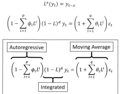
To represent this equation in an elegant way, a lag operator is used. Multiplying an observation by the lag operator will shift the observation backwards in time by a single time step. This is represented by Equation 4, while Equation 5 denotes the general forecasting equation of a non-seasonal ARIMA model. Figure 3-2 breaks down Equation 5 into the three components of the ARIMA model.

Lx(yt) = yt-, (4)

p q

1 -1 L' (1 - L)d yt = 1 + O L Et (5)

Autoregressive Moving Average

1 y =( 1+ > L' et

1 jrtd1=1

Integrated

3.1.1 Stationarity

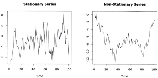
The ARIMA model requires the time series data to be stationary [12]. Stationarity is defined as a series of data with its mean, variance and autocovariance being invariant in time. Figure 3-3 illustrates the difference between a stationary and non-stationary series.

Stationary Sers Non-Stationary Series

0 20 40 60 so 100 0 20 40 60 so 100

Figure 3-3. Comparison between stationary and non-stationary series [12]

While the points in a series may not have constant properties over time, the difference of points in the series might. Hence, a non-stationary series can often be corrected by simple transformations such as differencing [ 12]. Differencing can help remove the trend or cycles within

the data.

In data with high seasonality, it is difficult to use purely differencing to remove the seasonal trend in the data. Furthermore, increasing the order of the AR or MA parts of the model may not be feasible. In such cases, a variant of the ARIMA model, seasonal ARIMA, is used to counteract the seasonal trends. Seasonal ARIMA has a total of six model parameters: (p, d, q) and (P, D,

Q).

parameters to describe the seasonal component. The seasonal parameters work in the same fashion but are applied by seasons rather than by time steps.

3.1.2 Model Fitting

After determining the various model parameters for the ARIMA model, the model is fitted to the data by computing the values of the weight coefficients in the forecasting equation. The two main approaches to determine the coefficients are non-linear least squares estimation and maximum likelihood estimation [9]. Maximum likelihood estimation is usually the preferred method. With an estimation of the coefficients, the model can then be assessed by different criteria to determine its accuracy. The procedure of optimization of the model is elaborated further in

Section 5.1.2.

3.2 MLP

The Multi-Layer Perceptron (MLP) is a simple feed forward neural network with multiple hidden layers. While not usually used in forecasting time series data, there has been some success using MLP with a specified time window in [5], [7]. The model architecture of a basic feed forward neural network can be customized to fulfill different functions other than forecasting such as classification and dimensionality reduction.

3.2.1 Neuron Structure

A neural network consists of many nodes or neurons that are intricately linked to each other.

It is a model inspired by basic neural elements of the human brain. Each neuron has a structure that consists of five components: input, weights, sum, activation function and the output [5]. The structure of a single neuron is depicted in Figure 3-4.

Input Weight

saWO _{Activation Fu ocklos}

X3 v43 X j Sn utu

Figure 3-4. Structure of an artificial neuron [13]

The inputs are basically the input data processed by the neuron. The inputs can both contain the actual data from the time series and a bias that has been applied to the neuron. The output depends heavily on the weights and activation function of the neuron. The output of the ith neuron is illustrated mathematically by Equation 6.

yi =- x wij (6)

(j=O

where there are n inputs with the bias represented by] = 0; a is the activation function.

The weights are all determined during the training stage of the model via backpropagation which will be covered in a subsequent section. The activation function is predefined as part of the model architecture and is usually dependent on the type of output expected. Several commonly used activation functions are sigmoid, arc-tangent, hyperbolic tangent, softplus, rectifier, and linear functions [14]. Activation functions cause the output to be within a certain range, such as rectifiers that range from 0 to +oo, the sigmoid function that ranges of 0 to +1 or the hyperbolic tangent function that forces the output to a range between -1 and + 1. The behavior of the activation

functions can be seen in Figure 3-5 where several commonly used non-linear activation functions are plotted.

-- sigmoid -- tanh - ReLU - SoftpluS 3 -I 2-1 0---21 -6 -4 -2 0 2 4 6 x

Figure 3-5. Commonly used non-linear activation functions [15]

Different activation functions are used for different purposes such as the softmax function in the output layer for classification problems and linear activation functions for regression problems.

3.2.2 MLP Model Architecture

With multiple neurons linked together, it forms a neural network. A simple feed forward neural network describes a network where the connections between neurons only flow in the forward direction. This is shown in Figure 3-6 where the direction of flow goes from the input (at bottom) to the output (at top) with each neuron linked intricately to other neurons. Each neuron is represented by a circle; the input nodes are not technically neurons as they forward the signal without any processing [5].

Output Layer

Hidden Layer

Input Layer

I t

Iti

Figure 3-6. A feed forward neural network with one hidden layer [5]

With each neuron representing a linear or non-linear function, depending on the chosen activation function, the network of neurons allows the model to accomplish complex tasks. In the context of forecasting, the model is able to establish the complex temporal relationships within the data. While more neurons and hidden layers would allow learning of more complex tasks, too many may result in overfitting of the model. Therefore, it is important to optimize the number of

3.2.3 Model Training

The learning process of the model is an optimization exercise to minimize a specified loss function by tuning the weight parameters of the neural network. Before optimization can begin, it is important to be able to measure the performance of the model. Depending on the loss function chosen, it can drastically affect the training result. Common loss functions include the mean absolute error (MAE) and the mean squared error (MSE) [5]. MSE measures the averaged squared distance between the true and predicted values, while MAE measures the averaged absolute distance.

The neural network is optimized through the use of an algorithm called gradient descent [5]. It involves computing the gradient of the loss function with respect to the weights and bias of the neurons. When the error gradient is determined with respect to the weight parameter, the weights are updated in the opposite direction of the gradient to minimize the error. This is defined by Equation 7 where 6' and 6 represent the updated and previous weights, L denotes the loss function and y is a scalar multiplier that represents the learning rate of the model.

OL(6)

()

d6

The gradients are computed through a technique called back-propagation, which is based on the derivative chain rule [5]. Hence, it is possible to see how the error from the loss function is propagated backwards to each preceding neuron layer.

This process is iterated several times (called epochs) over the training data to move the weight parameters closer to their optimum values, minimizing the loss function. With a large dataset, it becomes computationally infeasible to calculate the loss and gradient over the entire dataset [5]. Therefore, variants of gradient descent break the data into subsets called batches and

updates the weight parameters after each batch. Some variants include an additional parameter called decay that reduces the learning rate of the model as the weight parameters approach their optimum values [5].

A common problem often encountered in training a neural network is overfitting.

Overfitting occurs when the model tries to reduce the error by fitting a more complex model than required. This phenomenon usually results in a model that performs well on the training data but poorly on new data [5]. Overfitting can be prevented in several ways such as early stopping and dropout. Early stopping uses a small subset of the training data as a validation set which the model is not exposed to. After each epoch, the model is tested on the validation set and the error is determined. If the validation error starts to increase despite a decreasing training error, overfitting has occurred and the training is terminated early. On the other hand, dropout freezes a fixed percentage of connections in the neural network for each training epoch while the rest of the weight parameters are updated normally. This helps to prevent the overfitting of the model.

3.2.4 Forecasting in MLP

By customizing the number of nodes in the input layer and the number of neurons in the

output layer, the MLP is able to conduct both univariate and multivariate forecasts. In the univariate forecast, the number of input nodes will correspond to the number of lookback points while the number of output neurons will correspond to the number of lookahead points.

For the multivariate forecast, all the lookback points for each parameter is inputted into the model. This allows the model to learn the complex relationships between each parameter and between each lookback point. The output layer can be configured to either produce a single step forecast for each parameter or a single step forecast for one parameter.

3.3 LSTM - RNN

Recurrent neural networks (RNNs) differ from the basic feed forward neural network by having recurrent loops within the hidden layers. These recurrent loops enable RNNs to maintain a hidden state vector across time which acts as a memory of past information [5]. This makes it suitable for modelling sequential data. In recent years, RNNs have achieved "state-of-the-art performance in supervised tasks such as handwriting recognition and speech recognition" [4] which are both a form of sequential data.

3.3.1 Recurrence

A drawback of the MLP is that while it is able to account for the dependencies between

different time steps, it is unable to handle long term temporal dependencies in the data that range over hundreds of time steps [5]. Figure 3-7 depicts the recurrent loops in a RNN where the output of the previous time step affects the decision made in the current time step. This feedback allows the RNN to incorporate temporal dependencies of the data. This structure can also be represented

by unfolding the network in time as shown in Figure 3-7. The input and output data are represented

by x and h, respectively, while the internal state is denoted by s.

h ht-1 ht ht+1

V

sV

sVs

iUo

W

0 W

UU

U

U

Ut

tu

tru

tu

U, V and W are weight matrices between the input and hidden layers, hidden and output

layers, and hidden layers, respectively. The weight matrices are similar to a conventional neural network. It can be observed that the internal state vector is constantly updated with each time step, enabling it to retain a memory of all the previous points in the sequence [5]. Hence, the current output depends on all of the previous inputs. This allows RNNs to incorporate temporal dependencies in the data. The RNN structure can also be represented mathematically as shown by the two equations below. The same convention of variables is used as Figure 3-7. The neuron bias is denoted by b, while o- denotes the activation function.

st = Gr(Uxt + Wst_ 1 + bs) (8)

ht= a(Vst + bf) (9)

3.3.2 Model Training

Similar to the MLP, backpropagation and gradient descent is used to update the weight parameters to minimize the error of the loss function. However, now instead of backpropagating the error from just the output, there is a need to backpropagate the error through time. In theory, the algorithm should be able to learn and update the weights to put the right information into the hidden state memory. However, in practice, training RNNs is difficult and it is known that standard RNNs "perform poorly even when the outputs and relevant inputs are separated by as little as 10 time steps" [5].

The reason for the poor performance is due to the backpropagation through time and the model architecture. With the chain rule being applied multiple times in backpropagation, the gradients flowing through the network will either grow very large or decay to zero [3]. These problems are commonly referred to as the exploding and vanishing gradients, respectively. Hence,

3.3.3 LSTM Model Architecture

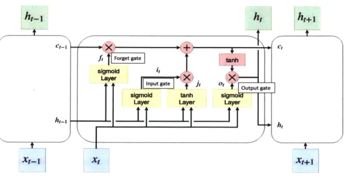
Several solutions have been proposed to solve the vanishing gradient problem by using gated RNNs. The Long Short Term Memory (LSTM) model is one such gated architecture that has proven to be effective in many practical applications [3]. Instead of a simple neuron structure, LSTM is made out of units or cells that have a more complicated structure. Figure 3-8 shows an example of a LSTM unit unfolded in time, similar to Figure 3-7. Gates restrict access to the memory state of each LSTM unit to remove the problem of vanishing gradients. There are a total of three gates in a typical LSTM unit: forget gate, input gate, and output gate.

ht-1

ht

ht+1

figu Forget gateM _tns

ot +output _{gate f}

sigmild tanm

Layer Layer Layer

Xt-1 Xt Xt+-1

Figure 3-8. LSTM unit with gated connections [3]

The memory state of the cell is denoted by c, whilef, i and o denotes the forget, input and output gate functions respectively. The gates control the manipulation of the memory state of the cell. This is achieved through the use of gate functions that have a value between 0 and 1. For example, a forget gate function value of 0 would cause the cell memory state to be totally forgotten while a value of 1 would keep the memory state as it is. The various functions in the typical LSTM

unit are shown mathematically in the following equations. The input and recurrent weight matrices for a LSTM unit are denoted by Wand R, respectively. Here, 0 is an operator that denotes element-wise multiplication, and a- represents the sigmoid activation function used in the LSTM unit.

t= tanh(Wxt + Rjht-1 + bj) (input) (10)

it = a(Wixt + Rjht 1 + bi) (input gate) (11)

ft = o-(Wrxt + Rfht_ + bf) (forget gate) (12)

ot = o(Woxt + ROht-1 + bo) (output gate) (13)

C=

it

h= tanh(ct) 0 ot (output) (15)

By having a fine control over the cell's memory state, LSTM is able to learn long term

temporal dependencies in the data efficiently. LSTM will be used interchangeably with RNNs throughout this thesis.

3.3.4 Depth in RNN

The idea of depth in LSTM is different than in MLP. MLP achieves depth by processing the input data through multiple hidden layers before producing an output [5], whereas LSTM achieves depth by maintaining a memory state of the past. This means that LSTM may not be able to model complex sequential data which requires hierarchical processing of information through multiple non-linear layers [5].

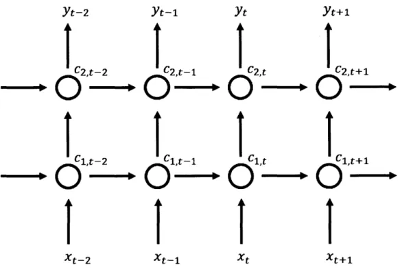
This can be resolved by using LSTM with multiple hidden layers, achieving both depth in time and in layers. Figure 3-9 illustrates this concept where many LSTM units are stacked in multiple layers similar to the MLP. The output of a LSTM unit is connected to the input of the next layer where y represents the final output.

Yt-2

I

Yt+1

Figure 3-9. Stacked LSTM structure with two hidden layers

3.3.5 Forecasting in LSTM

Even though each time step produces an output, only the output of the current time step is used as the one step forecast result. As both the input and output are in the form of vectors, it is possible to use LSTM for both univariate and multivariate forecasting. The complex relationships between the multiple parameters are learnt by the hierarchical learning process through multiple stacked LSTM layers.

3.4 Anomaly Detection Methodology

With one step forecasting, anomalies can be detected through the use of the distribution of residuals. Hypothesis testing is carried out to determine if a data point is anomalous based on its deviation from the actual data when compared to the residuals. Here, we assume that the residuals follow a Gaussian distribution; this assumption is discussed further in Section 5.1.6.

The predictive model is first exposed to a test dataset containing non-anomalous data. The Gaussian distribution of the residuals are then determined. Assuming that the residuals of the predictive model will follow the same distribution when exposed to an anomalous test dataset, the probability of the residual of a particular time step occurring in a given range can be calculated. This is also referred to as the p-value and it can be compared to a specified significance level to either reject or accept the null hypothesis.

3413% 34,13% 0.13% 2.14% 13.60% 13.60% 2.14% 0.13% -3s -2s -is 0 +Is +2s +3s 468,28%* *.--~95,6.46%m.* 99,73%a

Figure 3-10. Gaussian distribution [16]

Therefore, by setting threshold limits or a significance level as shown in Figure 3-10, an anomalous point can be determined when it falls outside of the confidence interval. For this thesis,

4 Experimental Setup and Dataset

To conduct anomaly detection on the given sensor data, three different predictive models are selected. Through experimentation, these models are first optimized before they are evaluated on their ability to detect anomalous patterns in the data. Section 4.1 describes the hardware and software involved in the experiment setup. It also outlines how the dataset will be partitioned into groups for training the neural network models. Moreover, it discusses the various preprocessing techniques used in preparing the data. The provided sensor data is then explored and shown in Section 4.2. This section also explains certain characteristics of the data as well as the anomalies present in the data. Subsequently, Section 4.3 details the partitioning of data to form the respective datasets for experimentation.

4.1 Experimental Setup

This section describes the process of setting up the experiments and preparing the data for the predictive models.

4.1.1 Hardware and Software

All experimentation and relevant code is programmed in R (version 3.5.1) [17]. The

ARIMA model is implemented using the Forecast package [18] while the neural network models are implemented using the Keras package [19]. All experiments were run on a machine with a 2-core CPU (Intel i7-4500U

@

4.1.2 Data Partitioning

To conduct the experiments, the available data is partitioned into four sets corresponding to their respective purposes: training, validation, test (forecast) and test (anomaly detection). The purpose of the training dataset is to select the best model parameters to infer the relationship between the input and output data. The validation dataset is used as a means to prevent overfitting of the model by early-stopping. The test dataset for forecasting contains data that exhibit the normal behavior while the test dataset for anomaly detection contains a mixture of data with normal and anomalous behavior. Hence, the first test dataset is where the distribution of residual errors is characterized. These parameters are then utilized to determine the anomalies in the second test dataset.

4.1.3 Preprocessing

As the inputs to the models have to be structured in a specific way, there is a need to preprocess the data. In particular, the neural network predictive models require the input data to be within the range of 0 and 1. Hence, a min-max normalization is applied to the data. There are two options of applying the normalization algorithm to the data: within each wafer cycle or to the whole dataset. As these anomaly detection algorithms are meant to be applied to an actual production setting, the normalization is done within each wafer cycle without any dependence on previous data.

Applying the normalization within each wafer cycle also helps to reduce the effects of level shifts or drifting behavior as shown in Section 4.2.2. However, if the extreme outlier occurs due to noise, it can detrimentally affect the accuracy of the forecasting.

4.2 Dataset

The provided dataset for experimentation originates from the Brookside server for the plasma etcher machine (OXLR7_LAMAL1). The Brookside server records a total of 31 parameters, a subset of the many parameters available from the machine. The entire dataset consists of two recipes (920 and 945) that were running on the machine when an unconfined plasma excursion occurred for the period of 2016-07-26 to 2016-08-02. This issue resulted in known anomalies identified in three specific parameters as shown in Table 4-1. All dates are in the format YYYY-MM-DD.

Table 4-1. Known anomalies and period of occurrence

No. Parameter Period of Anomaly Occurrence

5 BOT_RFRevPwrIn 2016-07-26 to 2016-08-02

17 ProcChmBotElecTempMon 2016-07-19 to 2016-08-02

19 ProcChmEndPtChanCIn 2016-07-26 to 2016-08-02

It can be observed that the anomalies from parameter 17 occurs prior to the unconfined plasma excursion which may be a possible early indicator for machine failure. More details on the physical significance of these three parameters can be found in Appendix A.

4.2.1 Anomalies

The anomalous patterns can be visually identified when compared to their expected normal behavior as shown in Figure 4-1. Each individual wafer cycle is plotted and overlaid to compare the patterns between the time series data.

60-.El 020-CO 0-Oe+00

..

J1611l1

I

A

I

(a) Parameter 5 - Normal

2.0-c E1.5 0 0. Ui ."1.0-0 E -t 005-0.0

Oe+00 le+05 2e+05 3e+05

Tune (c) Parameter 17 - Normal 8000-U ~000-E -r 1 00

0-Oe+00 le+05 2e+05 3e+05

(e) Parameter 19 - Normal

so- 60-cf40 -0 20-Oe+00 0-

I14iL1

Oe+00 le+05 2e+05 3e+05

Twne (d) Parameter 17 - Anomalous 30000-.E 3~0000-T

0-Oe+00 le+05 2e+05 3e+05

Time

(f) Parameter 19 - Anomalous

3e+05

U.

These anomalies present different levels of difficulty. Parameter 19 has the most significant difference with a large increase in amplitude and a total change in its pattern, making it possibly the easiest to detect. While parameter 17 is also distinctive, it has a lower drop in amplitude while still maintaining the general pattern for that particular recipe step. The hardest to detect would most likely be parameter 5. While it is visually distinct, it is a contextual anomaly that occurs within the operational range of that parameter. Furthermore, the randomly occurring spikes of noise may affect the ability of the model to detect the anomaly.

4.2.2 Characteristics of Data

Each ".rpt" file provided consists of one wafer cycle with 31 parameters. Each wafer cycle has a duration of approximately 300 seconds for recipe 920 and 150 seconds for recipe 945. Each cycle consists of approximately 600 and 300 timesteps for recipe 920 and 945, respectively. Each wafer cycle has a total of 8 recipe steps with the optical endpoint signal determining when the process in step 3 terminates. This accounts for the varying duration between each wafer cycle. Both recipes are similar and differ only in the duration of recipe step 3, where recipe 920 has nearly twice the duration of recipe 945. This is depicted in Figure 4-2 where we can observe that the general pattern remains the same with a different time length in recipe step 3, which constitutes the middle bulk of the process.

Cycle 8000- - 920 - 945 U 6000- 4000-E U U 0 200

0-Oe+00 le+05 2e+05 3e+05

Time

Figure 4-2. Difference between recipe 920 and 945 (Parameter 19)

The following subsections will explore certain special characteristics of the different parameters.

No Variation

Out of the 31 parameters, six of them do not exhibit any variation at all throughout the whole dataset. As there is no expected change, the six parameters (parameters 10, 11, 13, 20, 27 and 28) are excluded from the experiment. This is also due to the fact that data with no variation was found to significantly decrease the accuracy of the neural network predictive models. Hence, the experiments are done with 25 parameters in total.