Design and use of a large-format CCD instrument for the identification and study of distant galaxy clusters

DESIGN AND USE OF A LARGE-FORMAT CCD INSTRUMENT

FOR THE

IDENTIFICATION AND STUDY OF DISTANT GALAXY CLUSTERS

by

GERARD ANTHONY LUPPINO

B.S. Astronomy and Physics

The Pennsylvania State University

(1983)

SUBMITTED IN PARTIAL FULFILLMENT OF THE REQUIREMENTS FOR THE

DEGREE OF

DOCTOR OF PHILOSOPHY IN PHYSICS at the

MASSACHUSETTS INSTITUTE OF TECHNOLOGY August, 1989

@ Massachusetts Institute of Technology 1989

Signature of Author Department of Physics August, 1989 George R. Ricker Thesis Supervisor George Koster Chairman, Department Committee

SEP 1 2

1989

ARCHjvre

Certified by

DESIGN AND USE OF A LARGE-FORMAT CCD INSTRUMENT

FOR THE

IDENTIFICATION AND STUDY OF DISTANT GALAXY CLUSTERS

by

GERARD A. LUPPINO

SUBMT17ED TO THE DEPARTMENT OF PHYSICS OF THE MASSACHUSEITS INSTITUTE OF TECHNOLOGY ON AUGUST 1989, IN PARTIAL FULFILLMENT OF THE REQUIREMENTS FOR THE DEGREE OF

DOCTOR OF PHILOSOPHY IN PHYSICS ABSTRACT

This dissertation describes a search for distant clusters of galaxies (z>0.3). Cluster candidates were selected from a sample of radio sources with steep, low-frequency spectra since such radio sources are often found in rich nearby galaxy clusters. The steep-spectrum radio source (SSRS) is thought to be produced by the confinement of the radio plasma by the thermal pressure of a hot intracluster gas; therefore, we expect clusters discovered by this selection criterion to be bright x-ray sources and excellent targets for future x-ray satellites such as ROSAT, ASTRO-D and AXAF. These objects are also more likely to be true physical associations rather than the chance superpositions of galaxies that may plague some optically selected samples, particularly those at faint magnitudes. In order to identify the optical counterpart of the SSRS and see if the radio source was part of a distant cluster of galaxies, optical images to faint limiting magnitudes were required. Therefore, an imaging instrument incorporating mosaics of CCDs was designed and built . With this instrument, it is possible to observe faint, distant clusters of galaxies with spatial resolution limited by atmospheric seeing, while at the same time covering a relatively large field of view.

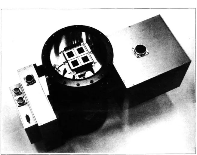
The major task in the creation of this instrument was the design and construction of two separate CCD camera systems; each based on different CCD mosaics. The first camera system incorporates four prototype, TI 850 x 750 virtual-phase CCDs (22.3 gim square pixels) arranged in a square pattern with the device packages abutted. The second camera system is designed to operate a four-chip CCD imager made by MIT Lincoln Laboratory. The imaging area of this CCD mosaic is 840 x 840 pixels (27 pm square pixels) formed by abutting four 840 x 420 framestore devices with seam losses less than 6 pixels. Details of the CCD camera electronics design as well as details of the mechanical design of the CCD cameras and LN2 dewars are described.

A total of 30 SSRS fields were observed with this CCD instrument mounted on the 1.3m and 2.4m telescopes of the Michigan-Dartmouth-MIT (MDM) Observatory on Kitt Peak. Additional CCD images of 5 of these radio sources were obtained with the Kitt Peak 4m telescope equipped with the KPNO prime focus CCD. Of these 30 SSRSs, 26 have been optically identified. In all, 15 of the observed fields contain visible clusters of galaxies, some of which are quite rich. Of the remaining 15 SSRSs, 6 are identified with faint galaxies , 2 are identified with poor groups, 3 are probably quasars, and 4 of the fields have uncertain or no optical counterpart. The median value for the estimated redshift of the 15 clusters is z=0.43 and the median richness is Abell Class 2. Nearly all of the radio sources have classical double-lobed morphology, and in half of the sources associated with clusters, the radio source is identified with a fainter cluster member rather than with the brightest cluster galaxy. In all cases where the cluster is BM Type I, however, the radio source is identified with the optically dominant galaxy.

Observations are also presented of three distant clusters that were not part of the radio selected sample: 0414+009, an x-ray bright BL Lac object coincident with the optically dominant galaxy in a Richness Class 1 cluster; 1217+1006, a compact group containing an extremely blue (B-R) ~ 0.0 object that may be either a QSO or a BL Lac; and 1358+6245, a new, x-ray luminous (Lx (0.5-4.5 keV) = 8.4x104 4 erg s-l), extremely rich (Richness Class 3 or 4), distant cluster of galaxies (z=0.323) which exhibits the Butcher-Oemler effect with a blue galaxy fractionfb = 0.18 orfb = 0.10 depending on the background galaxy correction.

ACKNOWLEDGMENTS

This instrument and scientific program would not have been possible without the help of a large number of people. First of all, I would like to thank my thesis advisor, George Ricker, who gave me access to a large number of CCDs and allowed me to use some of the best of them in this instrument. He also provided guidance and encouragement, and allowed me the freedom to be creative in the instrument design. I am also indebted to Ian McHardy and Brin Cooke, who developed this method for searching for distant galaxy clusters, and graciously accepted me as a collaborator. I appreciate the constructive comments and advice I received from my thesis committee members, Claude Canizares, and John Tonry. I am especially grateful to John, who taught me how to think as a scientist, and changed my perspective on instrumentation, urging me to "put the science first and let the science requirements drive instrument designs." John was always there to answer questions and help me wring the most out of my data. In addition, as the reader will later discover, nearly all of the software tools I use for data reduction in this thesis were developed and kindly provided by John. Also, thanks to Paul Schechter for helpful advice and criticism during the final stages of this project.

During my first three years as a graduate student, I worked closely with John Vallerga, who taught me almost everything I know about CCDs. The time I spent working with John was the most "productive fun" I ever had in the laboratory. And, I can never thank Roland Vanderspek enough. During my entire time at MIT Roland has been my best friend, companion, and advisor. He has helped me with virtually everything and I will be eternally grateful. I also appreciated the "baked goods" that often appeared when I was working on some particularly tedious or difficult problem.

The designs for much of the CCD electronics used in the instrument described later are based on original designs by John Doty. I first met John when I visited MIT 6 1/2 years ago, and he greatly influenced my decision to come to MIT to work in the CCD Lab (then the Balloon Lab). I have never regretted that decision. The Center for Space Research (CSR) CCD Lab has been a great place to work: partly because of the facilities, but mostly because of the people. I thank Mark Bautz and Pat Mock for relieving me of my responsibilities for the laboratory x-ray CCD system so that I could spend my time working on optical instrumentation and the scientific program for this thesis. Mark has also been an endless source of scientific advice and information about clusters of galaxies, and I appreciate the time he spent answering many of my questions. Pat not only helped me finish some unfinished electronic designs, he designed and built the hardware to interface the laboratory CCD cameras to our SUN and MicroVAX computers. Pat also went observing for me when I was too busy. Lawrence Shing and Ed Boughan deserve the credit for debugging the electronic design for the Lincoln Laboratory CCD system and actually constructing the circuits and making them work while I was busy writing this thesis. I have also enjoyed working with (as well as sharing a house with) George Mitsuoka (thanks for all the stargate) and Steve Rosenthal. A few years ago, I got my feet wet working at MDM Observatory when George and I upgraded the MASCOT with new CCDs and electronics. George also wrote MIDAS to interface the MASCOT to one of our old generic computers. Recently, Steve wrote the CCD tool program and ultimately interfaced the MASCOT and (later) the BRICC to the MDM Observatory SUN computers. I must also thank Mike Decker, who helped me sift through many TI-4849 CCDs while I was searching for the one to use in the BRICC, and Suzan DeFreitas who helped with much of the galaxy cluster data reduction and with the

construction of some of the instrument hardware. I thank Rosemary Hanlon for her help with some of the figures (and for dealing with Graphic Arts), and for her useful tips concerning WORD and the Macintosh. And thanks, Shep, for always making me laugh.

CSR machinists David Breslau and Leo Rogers were responsible for actually bringing the instrument design to life. During the course of construction, their excellent suggestions often improved the instrument design and their craftsmanship and attention to detail is evident in the final product. In addition, I am especially grateful to our CSR purchaser, Dan Calileo, who was always able to obtain the parts and services I required.

I would like to thank Barry Burke and his co-workers in Group 87 at MIT Lincoln Laboratory for their marvelous CCDs. I have enjoyed working with Barry and I am grateful for the education he has given me concerning some of the details of CCD design and manufacture. Barry was also kind enough to provide the photographs of the Lincoln Laboratory CCDs shown in Chapter 4. I am grateful to Stephanie Gajar for years of friendship and companionship. In addition, as part of the Lincoln Laboratory Group, she has been a source of useful information about these CCDs and she has served as a "CCD courier" between our group and Lincoln Laboratory. I would also like to thank the (former and present-day) CCD designers at Texas Instruments responsible for the TI-4849 and the TI 850 x 750 CCDs: Mark Wadsworth, Dan McGrath, Harold Hossack, and Jack Freeman.

The astronomers from University of Michigan, Dartmouth College, and MIT are fortunate to have an observatory (the MDM Observatory) staffed by outstanding people: Matt Johns (now at NOAO), Bob Barr and Larry Breuer. Special thanks to Matt for his excellent auxiliary instrumentation (the MIS instrument adaptor and intensified TV finder and guider) which were necessary for the proper operation of my CCD camera. Matt and Bob helped me debug the electronics at the telescope, and Bob is now responsible for the day-to-day maintenance of the instrument. He also fixes it when it breaks, and has mechanically adapted the CCD camera to the Observatory spectrographs. And thanks to Larry and Bob for cleaning the telescope mirrors before some of my observing runs. I'd like to thank the other astronomers with whom I've spent many productive (as well as cloudy) nights at the telescope: John Vallerga, Roland Vanderspek, George Ricker, Ian McHardy, Brin Cooke, Ed Ajhar, Pat Mock, Claude Canizares, Peter Vedder, John Tonry, and Mark Bautz. I must confess I've learned to love optical observing.

I would like to acknowledge the excellent astronomical education I received (both in and out of the classroom) as an undergraduate at Penn State. My good friend Jim McCarthy showed me how easy (and fun) it was to build a telescope and play in a machine shop. Larry Ramsey gave me my first opportunity to work with real optical instrumentation, and Gordon Garmire introduced me to high-energy astrophysics and gave me my first CCD to play with.

Finally, special thanks to Kristine for her love, support, patience, and good cheer. Well, it's finally finished. Here's what I've been doing for the last two years.

5

Table of Contents

C hapter 1 In trod u ction ... 9

Chapter 2 Clusters of G alaxies ... 13

2.1 Properties of Clusters of Galaxies ... 14

2.2 Standard Cosmology ... 19

2 .3 C osm ological Tests... ... 26

2.4 Galaxy Evolution in Distant Clusters ... ... 31

Chapter 3 Searching for High Redshift Galaxy Clusters... 39

3.1 Optical Searches for Distant Galaxy Clusters... 39

3.2 Steep-Spectrum Radio Sources and Clusters of Galaxies... 43

Chapter 4 Large-Format CCD Instrument Design ... ... 48

4.1 Instrument CCDs ... ... 49

4.2 Camera System Design for Four TI 850 x 750 CCDs... 51

4.3 Camera System Design for the MIT-LL 840 x 840 CCD... 68

Chapter 5 Instrument Performance ... ... 76

5.1 CCD Selection and Characterization Methods ... ... 76

5.2 CCD Selection and Optimization ... ... 81

5.3 Instrument Photometric Calibration ... ... 89

Chapter 6 Observations and Analysis of the Steep-Spectrum Radio Source Sample ... 93

6.1 Instrument Development and Cluster Observations ... 93

6.2 Data Acquisition, Reduction and Analysis Techniques ... 95

6.3 Optical Identification of Steep-Spectrum Radio Source Fields.... 96

6.4 Additional Non-Radio-Selected Cluster Fields ... ... 119

6.5 Analysis of Steep-Spectrum Radio Sample Properties ... 121

6 .6 Sum m ary ... ... 129

Chapter 7 Cl 1358+6245 at z=0.32 an X-ray Selected, Distant, R ich C luster of G alaxies ... 133

7 .1 O b servatio n s... 133

7.2 Analysis of Cluster Properties... 136

7.3 Discussion ... 157

C h ap ter 8 F u tu re W ork ... 17 1 8.1 Future Cluster Observations .. ... ... 171

List of Figures

FIGURE 2.1 CCD Image of the Corona Borealis cluster of galaxies...

FIGURE 3.1 CCD Image of the extremely rich cluster 0939+47 at z=0.4...

FIGURE 4.1 4.2 4.3 4.4 4.5 4.6 4.7 4.8 4.9 4.10 4.11 4.12 4.13 4.14 4.15 4.16 FIGURE 5.1 5.2 5.3 5.4 5.5 5.6 FIGURE 6.1 6.2 6.3 6.4a 6.4b 6.5a 6.5b FIGURE 7.1 7.2 7.3 7.4 7.5 7.6 7.7 7.8 7.9 7.10 7.11 7.12 7.13 FIGURE 8.1 8.2 8.3

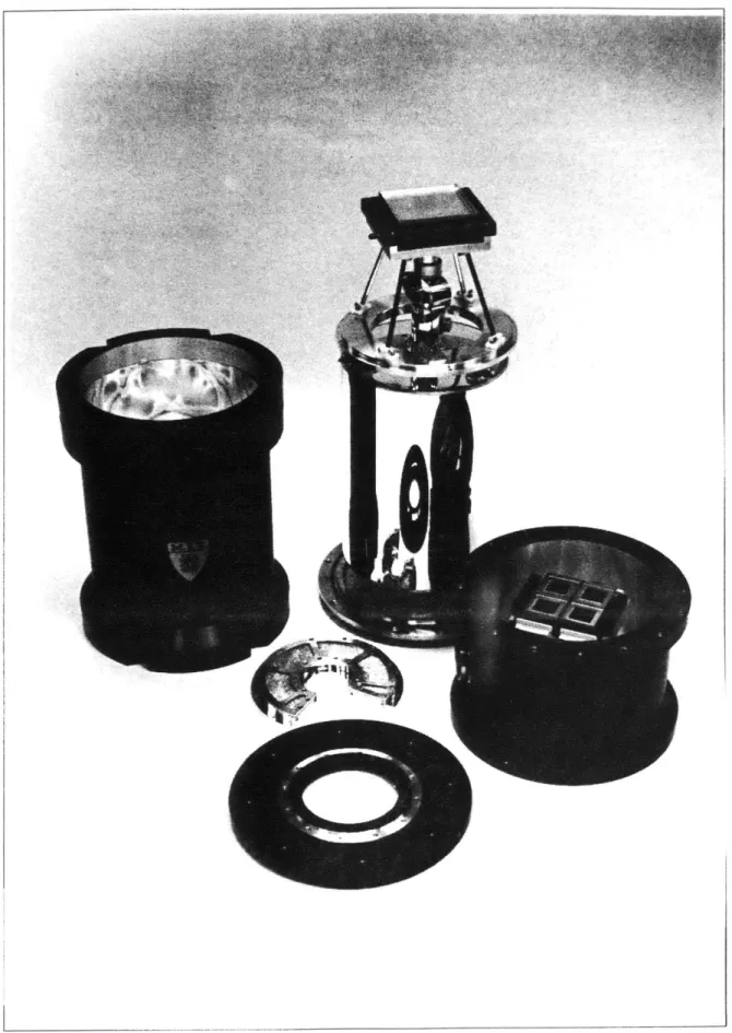
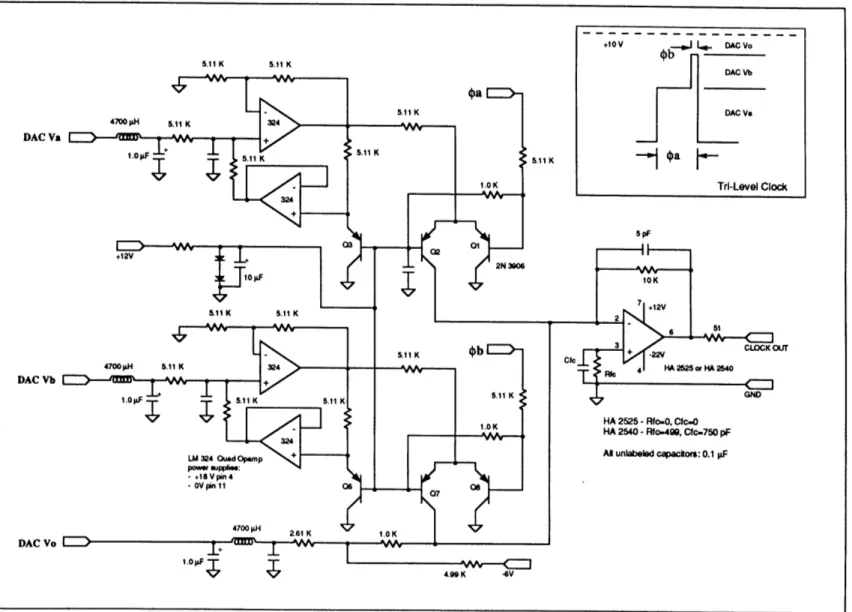
TI 850 x 750, TI 4849 and LL-CCID7 CCIs... TI 850 x 750 four-CCD mosaic... ... Side-mount dewar and TI-4849 camera head... Large-format CCD coaxial dewar - assembly drawing ... .. Internal view of dewar with TI 850 x 750 four-CCD mosaic ... D ew ar -exploded view of parts... External view of CCD dewar and electronics boxes... CCD control electronics -VPCCD -block diagram... Virtual-phase CCD timing diagram for tri-level delta clocking... T ri-level clock driver circuit... Transversal filter CDS circuit and 16 Bit A/D circuit ... ... Lincoln Laboratory 840 x 840 CCD mosaic... ... Closeup photo of LL 840 x 840 CCD mosaic... Micrograph of the LL 840 x 840 gaps... Internal view of dewar with LL 840 x 840 CCD mosaic ... CCD control electronics -3PCCD -block diagram... T I-4 849 x-ray histogram ... TI-4849 linearity... TI 850 x 750 mean-variance curve . ... T I 8 5 0 x 7 50 lin earity ... Flat fields for the TI-4849 and the TI 850 x 750 CCIs... Instrument photometric bandpasses... CCD images of distant clusters of galaxies ... ...

VLA maps of distant clusters of galaxies... R apparent magnitude as a function of redshift... Histogram of radio source-optical ID separations ... ... Correlation of richness vs. spectral index ... Radio luminosity vs. spectral index ... Optical ID apparent magnitude vs. radio flux (1411 MHz)...

Spectrum of Cl 1358+6245 central galaxy ... ... CCD image of Cl 1358+6245 ... Contour plot of Cl 1358+6245... ... Contour plot of the core of Cl 1358+6245 ... Galaxy surface number density contour plot... Luminosity function ... ... Galaxy spectral energy distributions (SEDs)... (V-R) vs R color-magnitude diagram... (B-R) vs R and (R-I) vs R color-magnitude diagrams... (B-R) vs (V-R) and (V-R) vs (R -I) color-color plots... R adial distribution of galaxy colors... Galaxy radial curve of growth and (B-V)rf color histogram... Central galaxy surface brightness image and contour plot...

X-ray histogram for a LL CCID-7 CCD... Instrument reducing optics assembly drawing ... Proposed designs for future large-format abuttable CCIs...

50 52 54 56 59 60 61 63 64 66 67 69 70 71 72 74 78 82 85 86 87 90 107 112 123 124 124 128 128 137 139 140 141 142 144 146 148 149 150 151 154 160 173 175 178

List of Tables

TABLE 3.1 Distant Abell clusters and other well-studied clusters at redshifts z>0.3...

TABLE 4.1 Thermal properties of dewar materials...

TABLE 5.1 5.2 TABLE 6.1 6.2 6.3 6.4

6.4

Measured performance of instrument CCDs ... System efficiencies ...

Sum m ary of observations... Steep-spectrum radio source positions and optical IDs... Properties of non-radio-selected clusters... Properties of non-radio-selected clusters of galaxies ... X-ray sources in observed steep-spectrum radio source fields...

Photometry of Cl 1358+6245 cluster galaxies... Galaxy counts in the field of Cl 1358+6245 ... ... Summary of the properties of Cl 1358+6245 ... ...

TABLE 8.1 Image scale and field of view for instrument CCDs with reducing optics... 41 58 83 91 94 98 126 120 127 161 144 156 174

To my Family:

Chapter

1

Introduction

Rich clusters of galaxies provide astronomers with some of the most powerful tools for measuring the global features of our universe. Numerous cosmological tests (such as the magnitude-redshift test, angular-size-redshift test, and Sunyaev-Zel'dovich effect) can be applied to distant clusters to try to ascertain the correct universe world model. Unfortunately, the luminosity and dynamical evolution of the galaxies in these clusters presents observational cosmologists with a formidable problem: cosmology and evolution appear to be inextricably tied together, and evolution must be understood before useful cosmological information can be extracted from measurements of distant clusters. Study of these problems requires a large sample of rich clusters of galaxies at moderate to high redshifts (z>0.2) where cosmological effects start to become important, and where cluster galaxy populations can be observed at different look-back times.

Until recently, only a handful of distant clusters have been studied in great detail, since normal galaxies at high redshift are extremely faint, and distant clusters of galaxies are not easy to find. The best known and well-studied sample of clusters is the Catalog ofRich Clusters of Galaxies by Abell (1958), which includes 2712 clusters, of which only 8 are at redshifts greater than z=0.3 (from the -600 with known redshifts). Many of the currently known distant clusters were serendipitous discoveries found by searching deep optical photographic plates (Kron, Spinrad and King 1977; Koo 1981), or by searching the fields of bright radio galaxies and QSOs (Spinrad and Djorgovski 1986). One would ideally prefer a distant cluster population which was systematically selected and not associated with some exotic object. Such a sample has been optically selected by Gunn, Hoessel, and Oke (1986), and contains 418 distant clusters, with redshifts ranging from 0.15<z<0.92 (for the number that have measured redshifts).

McHardy and Cooke (1989) have suggested that one might also find distant, rich clusters of galaxies in fields containing low-frequency (38-178 MHz), steep-spectrum1 radio sources, since there is a well established correlation between such sources and nearby rich clusters (Slingo 1974; Roland et al. 1976; Burns 1989). This method should not be particularly sensitive to selection effects since the physical mechanism producing the steep-spectrum radio emission is not associated with some exotic object, but originates from the confinement of the radio source by the thermal pressure of hot intracluster gas (Slingo 1974; Guthrie 1977). The clusters in this sample are also likely to be bright x-ray sources, and excellent targets for the ROSAT, ASTRO-D, and

1 The non-thermal radio spectra of extragalactic radio sources is well-characterized by a "power law," where the flux density per unit frequency interval is proportional to the frequency to some power i.e. Sy oc v-a. Steep-spectrum radio sources have aX>1.5, whereas "normal" radio sources have a-0.8.

AXAF, since the same intracluster gas responsible for confining the radio source is expected to be a copious emitter of thermal bremmstrahlung.

A large number of suitable steep-spectrum radio sources (SSRS) from the 4C and Culgoora catalogs were mapped by McHardy using the VLA to provide precise source positions for deep optical imaging (McHardy and Cooke 1989). In order to confirm the presence of a cluster at the radio position, and to study the properties of such clusters, deep optical images of the VIA fields were required. The imaging detector used for these observations must have enough resolution to allow optimal spatial sampling of the stellar seeing disk; only then will it be possible to reliably classify faint objects as stars or galaxies. The detector must also have a relatively large field of view since even very distant clusters often have large angular sizes1.

The high quantum-efficiency, linearity, and large dynamic range of charge-coupled devices (CCDs) make them the detector of choice for observing faint objects such as high redshift cluster galaxies. Currently available (single) CCDs, however, do not meet both of the requirements mentioned above. If the pixel size is optimally matched to the seeing, the field of view is too small. If too large a field of view is mapped onto a single CCD, it becomes impossible to adequately separate stars from faint galaxies. This thesis describes the design and construction of a sensitive, large-format, CCD imaging instrument which incorporates mosaics of CCDs. With this instrument, it is possible to observe faint, distant clusters of galaxies with spatial resolution limited by the atmospheric seeing, while at the same time covering a relatively large field of view.

The major task in the creation of this instrument was the design and construction of two separate CCD camera systems, each based on different CCD mosaics. The first of these camera systems incorporates four TI 850 x 750 virtual-phase CCDs (22.3 pm square pixels) arranged such that the device packages are abutted. These CCDs suffer from low-level charge transfer problems and have readout noise levels of 18-20 electrons rms. The second camera system is designed to operate a high-performance 840 x 840 CCD mosaic designed and built at MIT Lincoln Laboratory2. This hybrid imager is formed by abutting four 840 x 420 framestore CCDs (27 grm square pixels) with seam losses less than 6 pixels. These CCDs are three-phase devices with excellent charge-transfer properties and a readout noise levels of 2 electrons rms. The camera system has been designed to operate both the thick, frontside-illuminated and the thinned, backside-illuminated versions of these sensors.

1 The characteristic size of a cluster of galaxies is the Abell radius, RA, which equals 3 megaparsecs (Mpc). At z=0.5, this radius subtends an angle 6A, of 422 arcseconds, and at z=1.25, 6A=3 5 0 arcseconds. In fact, for a Friedmann cosmology with qo>0, the angle subtended by fixed metric length goes through a minimum at z=1.25 (see Chapter 2, §2.3b), thus the Abell radius for distant clusters will always have an angular size OA>6 arcminutes. The above calculation assumes a standard Friedmann cosmology with values of HO = 50 km s-1 Mpc-1 and qo=1/2

for the Hubble constant and the deceleration parameter, respectively.

We observed the distant galaxy cluster fields with this CCD instrument mounted on the 1.3m and 2.4m telescopes of the Michigan-Dartmouth-MIT (MDM) Observatory on Kitt Peak. The bulk of the observations for this dissertation were carried out while the instrument was still under construction.

In the following chapters, we describe the design of the large-format CCD instrument, and discuss the results of observations carried out with this instrument. We will start by reviewing, in detail, the properties of clusters of galaxies, and we will describe some cosmological tests that can be applied to high-redshift clusters, and briefly discuss the problem of cluster galaxy evolution. In Chapter 3 , we will discuss methods for finding high redshift clusters, and explain why a low-frequency, steep-spectrum radio sources is often a good indicator of the presence of a rich cluster of galaxies. In Chapter 4, we describe the CCD instrument design including the specifics of the mechanical design of the camera heads and dewars, and the details of the electronic controllers. The selection and characterization of the CCDs, and the photometric calibration of the instrument is presented in Chapter 5.

The observations of the distant galaxy cluster fields are summarized in Chapter 6. In addition, we also describe the new distant clusters and their optical and radio properties. In Chapter 7, we present the results of detailed BVRI photometry of Cl 1358+6245, the most spectacular cluster of galaxies in this investigation. This cluster is not part of the steep-spectrum radio sample, but was discovered with the Einstein observatory.

Finally, in Chapter 8 we outline future plans for cluster observations, instrument modifications, and CCD improvements.

REFERENCES:

Abell, G.O. 1958, "The Distribution of Rich Clusters of Galaxies," Ap.J. Supp., 3, 211.

Abell, G.O., Corwin, H.G., and Olowin, R.P. 1989, "A Catalog of Rich Clusters of Galaxies," Ap.J.Supp., 70, 1. ACO

Baldwin, J.E., and Scott, P.F. 1973, "Extragalactic Radio Sources with Steep, Low Frequency Spectra,"

M.N.R.A.S., 165, 259.

Bums, J. 1989, "The Radio Properties of cD galaxies in Abell Clusters I. An X-ray Selected Sample," Preprint

Gunn, J.E., Hoessel, J.G., and Oke, J.B. 1986, "A Systematic Survey for Distant Galaxy Clusters," Ap.J., 306, 37.

Guthrie, B.N.G. 1976, "A Search for Steep Low-Frequency Radio Spectra Among Quasars and Clusters of

Galaxies," Astrophys. and Space Science, 46,429.

Kron, R., Spinrad, H., and King, I. 1977, "Observations of a distant cluster of galaxies," Ap.J., 217, 951.

McHardy, I. and Cooke, B. 1989, in preparation.

Roland, J., Veron, P., Pauliny-Toth, I., Preuss, E., and Witzel, A. 1976, "Radio Sources and Clusters of Galaxies," Astron.Ap., 50, 165.

12

Slingo, A. 1974, "Observations of Ten Extragalactic Radio Sources with Very Steep Spectra," M.NR.A.S., 166, 101.

Slingo, A. 1974, "The Structure and Origin of Radio Sources with Very Steep Spectra," M.N.R.A.S., 168, 307.

Spinrad, H. 1986, "Faint Galaxies and Cosmology," P.A.S.P., 98, 269.

Spinrad, H., and Djorgovski, S. 1987, "The Status of the Hubble Diagram in 1986," in IAU Symposium 124, Observational Cosmology, ed. Hewitt, Burbidge, and Fang (Dordrecht Reidel), p. 129.

Chapter

2

Clusters of Galaxies

Clusters of galaxies are among the largest known objects in the universe. They often occupy a region of space in excess of three megaparsecs in diameter and contain hundreds to thousands of visible galaxies. Other than quasars, bright active galaxies, and the cosmic microwave background, large clusters are among the few objects that can be seen at great distances (at redshifts greater than one); they therefore provide observational astronomers with tools for studying the large scale distribution of matter and the properties of galaxies at earlier epochs. A study of the properties of clusters of galaxies may help answer questions concerning the origin and evolution of the universe. Clusters of galaxies are also very interesting objects in. their own right: they are dynamical laboratories where one observes evidence for dark matter, they are known to act as gravitational lenses (Soucail et al. 1988; Lynds and Petrosian 1989), and they may trace out the density fluctuations in the early universe that led to their collapse.

Rich clusters of galaxies were first discovered as pronounced enhancements of the surface number density of galaxies on optical photographic plates. Although clusters are also often bright x-ray sources (thermal

bremsstrahlung from hot, low density intracluster gas) and radio sources (nonthermal synchrotron emission from discrete sources associated with a member galaxy of the cluster), a cluster of galaxies is still classified and defined primarily by its optical properties. This chapter will review these optical properties of clusters of galaxies, as well as briefly discuss their x-ray and radio characteristics, and explain how distant clusters can be

used to measure the global features of the universe.

Section 2.1 describes the classification of clusters of galaxies, and briefly reviews their optical, x-ray and radio properties. Particular attention is given to some of the characteristics that will actually be measured for a number of clusters in this thesis. Since high-redshift, rich clusters are used as probes to measure various properties of the universe world model, the relevant equations of the standard Friedmann cosmological model used throughout this thesis are presented in Section 2.2. Although various forms of these equations can be found in most textbooks (Weinberg 1972; Peebles 1971), they are presented here, using a standard system of notation, for completeness, and with emphasis on the observables. Section 2.3 describes, in detail, some cosmological tests that rely on measurements of properties of rich clusters of galaxies, and Section 2.4 briefly addresses the subject of galaxy evolution in distant clusters, and the current problems evolution presents for cosmological interpretation.

2.1 Properties of Clusters of Galaxies

a) Catalogs

Most of what is known about clusters of galaxies has been derived from the study of the relatively nearby objects included in the two largest and best known catalogs: the catalog of Rich Clusters of Galaxies by Abell (1958) which contains 2712 very rich members, and the far more extensive Catalogue of Galaxies and of Clusters of Galaxies by Zwicky et al. (1961-1968). These researchers have developed methods to measure and classify clusters based on their sizes, shapes, galactic content, distance, surface number density profile (contrast), and luminosity function: properties that often provide one with clues about the physical environment of the cluster.

Since galaxy clustering ranges from small, irregular groups of a few galaxies, to large, dense aggregates containing thousands of members, it is difficult to define unambiguously what is meant by a cluster (and particularly a rich cluster) of galaxies. The inclusion of a cluster in a catalog is dependent on the selection criteria used to define the catalog. Abell specifically searched for rich clusters: to be included in the catalog, a cluster had to have: 1) at least 30 galaxies in the magnitude range defined by m3 and m3+2 where m3 is the magnitude of the third brightest cluster galaxy; 2) these 30 galaxies (or more) had to be contained within a

3.0h50-1 Mpc radiusl circle; and, 3) the estimated redshift of the cluster (based on the magnitude of the tenth brightest galaxy, mjo, had to be between 0.02<z<0.20. Abell only selected clusters from declinations north of S=-270 and in regions not known to be obscured by our galaxy. Zwicky's criteria were less restrictive and that catalog therefore contains many more entries: a total of 9134 clusters. For a cluster to be included in Zwicky's catalog, it had to have: 1) at least 50 galaxies within the magnitude range defined by mi and m1+3; and, 2) these 50 galaxies had to be contained within the contour where the galaxy surface number density fell to twice the background density. No distance limits were placed on Zwicky's clusters. The clusters in both of these catalogs were discovered on photographic plates from the 1.2m Schmidt telescope of the Palomar Observatory. The plates were taken while compiling the original Palomar Observatory Sky Survey (POSS).

The southern hemisphere extension of the Catalog of Rich Clusters of Galaxies has recently been completed by Abell, Corwin and Olowin (1989; ACO), using the UK 1.2m Schmidt telescope with IIIaJ plates. Galaxy clusters were selected using essentially the same criteria as Abell (1958). The ACO catalog contains 1635 clusters at declinations less than 8=-170, and includes clusters in the 5=-170 and S=-270 overlap region with Abell clusters. The all-sky catalog of rich clusters of galaxies now contains 4073 members. ACO have also revised the northern catalog; they have updated the coordinates to E1950.0 and E2000.0, and they have included Bautz-Morgan types (see below) and redshifts where known.

Vw

4

9,

4W

a

.4

A CCD image of the core of the Corona Borealis cluster of galaxies (Abell 2065) illustrating some of the morphological characteristics of galaxy clusters discussed in this chapter. This regular cluster is at a distance of - 430 Mpc (z = _{0.072) and is Bautz-Morgan type II. Only the central 700 kpc of the}

cluster is shown on the CCD frame. Abell counted 109 galaxies in the magnitude range defined by m3 and m3 + 2 within one Abell radius (- 3Mpc), placing this cluster in richness class 2. This image is a 600 second exposure in R-band obtained on a 1.3m telescope with a single TI 850 x 750 CCD in the instrument described later in this thesis. The plate scale is 0.47 arcseconds/pixel (North

is up and East is to the left).

0Sr

oil

Abell (and ACO) attempted to exclude clusters at distances greater than z=0.2 (since these faint clusters would be very sensitive to selection effects and would be difficult to identify in any case from photographic plates). Nevertheless, the Abell catalog does contain a number of clusters at redshifts greater than this limit (see §3.1). A catalog of very distant clusters of galaxies has been published by Gunn, Hoessel and Oke (1986; GHO). During the course of the preparation of this distant cluster catalog, GHO used hypersensitized photographic plates, image intensifiers coupled to photographic plates, and ultimately, CCDs to detect 418 faint clusters at

redshifts out to at least z=0.92. There is only slight overlap with Abell and Zwicky clusters. More will be said about these distant clusters in the following chapter.

b) Morphological Classfication

The Bautz-Morgan (1970) classification system for clusters of galaxies is based on the apparent contrast of the brightest cluster galaxy relative to the fainter cluster members. BM Type I clusters are dominated by a single, luminous, central galaxy which is often a cD galaxyl. BM Type II cluster have more than one giant elliptical of comparable brightness, and BM Type III clusters have no dominant galaxy. BM Types I-II and 11-III are intermediates between the above cases. The Bautz-Morgan type of a cluster can be determined quantitatively using the method of Dressler (1978). The magnitudes of the first, second and third brightest cluster galaxies are used to form the quantity A (m2-mj) + (m3-m). The cluster is then classified according to the value of A: BM type I clusters have A > 2.25 mag; BM type II clusters have 2.25 > A > 1.03 mag; and, BM Type III clusters have A < 1.03 mag. See Dressler (1978) for details.

An alternative, popular morphological classification scheme is the revised Rood-Sastry (RS) system (Struble and Rood 1982) based on the arrangement of the ten brightest cluster galaxies. There are six RS classifications arranged in a forked sequence: RS type cD -cluster has a supergiant, dominant galaxy with extended enveleope (very similar to BM type I); RS type B -cluster has two close, supergiant galaxies; RS type C -core-halo arrangement of the ten brightest, centrally located galaxies; RS type L -elongated, line arrangement of brightest galaxies; RS type I -irregular, or clumpy distribution with no well-defined center; and RS type F -flattened configuration often with numerous subclumps.

Various authors have correlated cluster features (e.g. x-ray luminosity, richness, and average separation of central galaxies -to name just a few) with both the BM and RS types. The BM system still appears to be the most popular and widespread, especially since clusters in the BM system are ordered in a monotonic, rather than a forked, sequence.

I

embedded in a gigantic, low-surface brightness halo that may extend as far as 1 Mpc from the galaxy center. Other than galaxies with active nuclei (e.g. QSOs and Seyferts), cD galaxies are the most luminous galaxies known. They are found at the centers of compact clusters, and they often have double or multiple nuclei. It is believed that cD galaxies may be produced by mergers of galaxies within the cores of rich clusters.

c) Richness and Galaxy Content

The richness of a cluster is a measure of the number of galaxies within a cluster. In his catalog, Abell (1958) classified cluster richness based on the number of galaxies, NA, counted within one Abell radius, RA, in the magnitude range defined by m3 and m3+2 where, again, m3 is the magnitude of the third brightest cluster

galaxy. There were 6 Abell richness classifications: richness class 0 - 30 5 NA 5 49; richness class 1 - 50 NA 5 79; richness class 2- 80 5 NA 5 129; richness class 3 - 130 5 NA 5 199; richness class 4 - 200 5 NA 5 299; and richness class 5 -- NA > 300. The Abell richness is largely independent of distance, but richness estimates for the z>0.2 clusters are often wrong, since the clusters were just too faint for Abell to get accurate count information. For example, cluster A851 was listed as a Richness Class 1 object (albeit very distant) but subsequent spectroscopic observations by GHO show this object to be extremely rich at z=0.4 (although Gunn argues that Abell may have identified a foreground group in the field, and not the z=0.4 cluster, see Figure 3.1). Another example is A370 which is listed as Richness Class 0; this cluster is actually Richness Class 3 (Kristian, Sandage and Westphal 1978; KSW), but it is quite distant at z=0.37.

Bahcall (1981) described an alternative method for determining the cluster richness, as well as the central galaxy density which is defined as the number of galaxies, N0.5, in the magnitude range defined by m3 and

m3+2 projected within a 0.5h50- 1 Mpc radius of the cluster center. It turns out that this number, corrected for

background and cluster richness, is strongly correlated with the velocity dispersion in the cluster (Bahcall 1981). This correlation will be used in later chapters to estimate the velocity dispersion of clusters for which there is no spectroscopic data.

d) Optical Luminosity Function

The luminosity function for a cluster of galaxies describes the distribution of luminosities of the galaxies in the cluster. As stated by Schechter (1976), luminosity functions can be obtained for any subclass of objects which can be identified by criteria other than luminosity. Two different luminosity functions are often mentioned: the integrated luminosity function N(L) which is just the number (or number density) of galaxies with luminosity greater than L, and the differential luminosity function n(L)dL which is the number (or, again, the number density) of galaxies with luminosities in the range L to L + dL. Clearly, n(L) = -dN(L)/dL.

The following analytic expression for the differential luminosity function was proposed by Schechter (1976)

n(L) dL = N * (L /L* )a exp(- L/L* ) d(L/L* ) . (2.1.1)

It can be interpreted as a power law, (L/L*)a, for the faint galaxies (L<<L*), and an exponential which dominates for the bright galaxies (L>L*). The region where n(L) changes rapidly is called the break in the

6I ,Mll

. III l t __ll i a l ll

18

luminosity function, and is characterized by the parameter L*. Schechter (1976), and more recently, Lugger (1986) showed that the value of L* is nearly the same for rich clusters of galaxies with an equivalent value, MV* - -21.5 + Slogh5O and a power-law slope of a=-1.25. Since M* appears to be constant, it has been suggested that it could be used as a standard candle; by measuring m*, one could directly measure the distance to a cluster (Schechter and Press 1976). This will be discussed further in §2.3.

e) x-ray emission

Clusters of galaxies have been known to be sources of x-rays since the late 1960's when x-ray emission was seen coming from M87 and the Virgo cluster. This cluster was the first extragalactic object seen in x-rays. In the next decade, the x-ray satellites Uhuru, OSO-7, Ariel V, SAS-3, OSO-8 and HEAO-A confirmed that many nearby, rich clusters were bright x-ray sources with luminosities in the range of 1043 to 1045 ergs/s: . In fact, clusters of galaxies are among the most luminous x-ray sources in the universe. The emision mechanism for these spatially-extended sources was eventually determined to be thermal bremmstrahlung from hot (108 K), low density (10-3 cm-3) gas which filled the volume between the galaxies and had a mass approximately equal to the mass of all the stars in the galaxies that make up the cluster. The thermal interpretation was supported by observations of x-ray line emission from iron, which also indicates the intracluster gas originated in stars and was somehow ejected from the galaxies in the cluster. A recent review of the physics and observations of x-ray emission from clusters of galaxies is given in by Sarazin (1986).

f)

Radio emission from clusters of galaxies is non-thermal synchrotron radiation due to the interaction of relativistic electrons with an intergalactic (or intragalactic) magnetic field. The source is usually associated with an individual galaxy, often one of the brightest optical galaxies, near the center of the cluster (McHardy 1979). A large fraction (-20%) of all extragalactic radio sources are in clusters of galaxies, but this may be simply explained by the fact that giant ellipticals, which occur preferentially in rich clusters rather than in the field, are the major class of strong radio galaxies (McHardy 1979). McHardy (1978) also found that strong radio sources were more likely to be found in x-ray luminous clusters. The intracluster gas that is known to be present from x-ray observations has an effect on the morphology and spectrum of the radio emission. Cluster radio sources have trail or distorted morphology indicating the interaction of a convential double-lobed radio source with the intracluster gas (Miley 1980). Radio sources in clusters also have steeper spectra: a > 1.2 (where Sy c v-a) for sources in clusters, whereas a - 0.8 for sources in the field. It is this property of clusters that serves as the selection criterion for the distant clusters in this thesis. The details of this selection method and the physical models for the radio emission are discussed fully in the next chapter.

19

2.2 Standard Friedmann Cosmology

a) preliminaries

The standard world model used throughout the following discussions assumes a globally homogeneous, isotropic universe correctly described by the equations of general relativity. In this universe, the most general possible line element is given by the Robertson-Walker metric (Sandage 1989 and references therein),

ds = c dt2 R (t) dr +r d +r sin Od p (2.2.1)

1k2

where the coordinates are comoving, R(t) is the universe scale factor (R(t) = 0 at t = 0), and k is a constant (+1, 0, or -1) that determines the spatial curvature of the universe. When the above metric is inserted into the Einstein field equations, along with the assumptions mentioned above, one obtains the two fundamental differential equations of cosmology (Weinberg 1972; Sandage 1961)

2 .2 R 2R 8,rG -kc 2 -+ R R" 2 +Ac .2 2 2 R 8rG -kc Ac - p (2.2.2) 2 3 2 3 R R

that describe the time evolution of the geometry of the universe. In these equations, p is the pressure of matter and radiation, p is the density of matter and energy, and A is the cosmological constant originally introduced by Einstein in an attempt to obtain a static universe that would have been impossible otherwise. Models with zero pressure and A=O are currently the most popular since they seem to describe the universe now. Only these models will be considered below. In this case, the Einstein equations reduce to

2 .. 2

R + 2R R = -kc (2.2.3)

*2 8 2 2

R- 8rGP R = -kc _(2.2.4)

3

Solutions to these equations will be discussed later in part d) where the time evolution of R(t) is discussed.

Equations relating the expansion factor R(t) to the redshift and other observables are presented below (note that all terms subscripted with 0 should be evaluated at the present epoch, i.e., now). These observables are the Hubble constant, H0, the deceleration parameter, q0, or density parameter, 00,

-1 = -1 (2.2.5) Ho=5R0(t)R

(t)=5Ro

qO= -Roo (2.2.6)

0o= *_8r GPo-2qO

PC 3H 2 (2.2.7)

Another important observable is the redshift, z, which is defined as z AA/X, or

1+z = -= - = (2.2.8)

A, v. R(t)

where the subscript o refers to the observed wavelength (or frequency), while the subscript e refers to the emitted wavelength (or frequency).

b) luminosity distance and angular size

Since all astronomical observations of distant objects rely on the detection of photons, it is necessary to consider the aspects of the propagation of light through the universe. The proper distance along a null geodesic (ds = 0) is obtained by integrating the Roberston-Walker metric (details of this integration are given in Weinberg

1972),

e dr _ c dt

o

.1-

yielding, for the comoving radial coordinate r, the expression (Mattig 1958)

r = 2 c q z + (qO - 1) ((1 + 2 q z) 1 . (2.2.10)

qO HO (1+ z)

The more useful term, however, is the luminosity distance, dL, which is defined so that it forces the bolometric flux f (in units of ergs cm-2 s-1) received from an object of bolometric luminosity L (in units of ergs s-1) to obey the inverse square law of flat Euclidean spacetime, i.e.,

4f L 2. _(2.2.11)

The luminosity distance can be related to the proper distance, which is only a function of the observables HO, qO, and z, by considering the true relation between observed flux and emitted luminosity. For small distances, spacetime can be considered to be locally flat, therefore

fo

measured in the emitter's frame by a factor of (1+z). Also, each arriving photon is redshifted in frequency by a factor of (1+z). When these two factors of (1+z) are included, the correct expression for the observed bolometric flux becomes

f,

47 r2 1 + z )2

It is obvious from this equation that the luminosity distance, as defined by equation 2.2.11, can be written as (Weinberg 1972)

dL= r (1 +z)= q2c q z + (qO - 1) ((1 + 2q₀z)1 1_1 - (2.2.13)

10H0

The above equation, which is exact for all z and qo, reduces to

d1 dL H 0[ C z + 21~1 -qO) z2.140)2 (2.2.14)

0

for small z. Note that this equation is exact for the two cases qO=O and 1 (Weinberg 1972).

Further cosmological effects must be considered when observing distant extended objects, such as galaxies at high redshift. Here, surface brightness becomes the limiting factor in the detection and study of these objects (Weedman and Williams 1987). Consider a galaxy of proper metric (comoving) diameter D. The observed angular diameter is then

(1+ z)D HO D gO (10+ z)

06(q , Z)= =--2 (22.5

8c 1Mpc qz +(qO - 1) (1+ 2q0z)1 ) (2.2.15)

where D is in units of Mpc if HO is in units of km s-1 Mpc-1. It is obvious from this equation that 0 can also be written as 0=(1+z)2D/dL. Therefore, one can also define an angular distance , dA, such that (Weinberg 1972)

d = = 2 . (2.2.16)

Observed surface brightness, Z, which is defined as observed flux per (observed) solid angle, can now be written as

2 _{2 2} L -₄ ergs cm-2 s-1 str- 1 (2.2.17)

6 41 D (1+ z)

where D is in units of Mpc as in equation 2.2.14. Notice that the surface brightness decreases as (1+z)4, which places severe limits on the detectability of normal galaxies with redshifts greater than unity (assuming distant galaxies are similar to nearby galaxies). This will be discussed in greater detail below and in the following chapter.

The expressions relating observed flux and emitted luminosity presented so far are only applicable to bolometric quantities (energy at all frequencies or wavelengths). In practice, observations are made in a finite bandpass, and the appropriate equations for monochromatic flux and luminosity must be used. In this

presentation, I will use notation similar to Gunn and Oke (1975) or Schneider, Gunn and Hoessel (1983 [SGH]), where any v or A subscript refers to an observed quantity, while an emitted quantity, which arises at a different frequency or wavelength in the emitters frame, has a subscript written in terms of the observed v or A. (using equation 2.5). The monochromatic energy flux is given by

Ly.,+z ) ergs cm-2 _s-1 _Hz-1

(2.2.18)

47r di

and

.= L y(14,> ergs cm-2 s-I

A-1

2

4

7rdi (1 + z)

The monochromatic surface brightness then becomes

L)(1+z) ergs cm-2 _s1

_A

(2.2.20)

41 2 5

4,rD (1 + z)

c) magnitudes

The apparent magnitude in filter i, of an object detected by a system with sensitivity Si(v) is defined as

m =-2.5log _fvSi(v)dv+C

0 (2.2.21)

and the absolute magnitude at the position of the galaxy (well, 10 pc away) is given by

,.aL v S (V

M = -2.5log 2 dv+ C

-0 4x d

do=10 parsecs.

Using equation 2.2.18 to replace the flux in equation 2.2.21 with the luminosity, one obtains expression for the apparent magnitude

Lv(1+z)(1+z m =2.5 log L S (v) dv + C 4 r d (2.2.22) the following (2.2.23)

Therefore, one can write,

L v(1+z 1+z)'Lv i m -M 2.5 log V(2+z) S (v) dv + C + 2.5 log 2 dv - C 0 4r d 04 do 4,r d L = 2.5 log 2 + 2.5 log 4 ir do fL v , i(v) dv (1+ z)f L( 1+ )S i (v) dv 0 JLVS (v) dv m - M.= 5log dL+ 25 - 2.5log(1+ z)+ 2.5log

L v(1+z) S i (v) dv

= 5logdL+25+K v(z) (2.2.25)

where dL is given in Mpc, and KVz) is the K-correction as defined in Oke and Sandage (1968) that accounts for the redshifting of the continuous energy distribution, Ly, through the fixed spectral response, Si(v) of the detector. The K-correction, as written above, is composed of two parts: the 2.5 log(1+z) term that accounts for

the change in bandwidth, and the wavelength dependent portion that is important if L[v] is not equal to L[v(1+z)]. For the case where the flux per unit wavelength, rather than unit frequency, is specified , the

difference between apparent and absolute magnitude is given by

JL

S.(A) dA

0

m - M = 5logd L+25+2.5log(l+z)+ 2.5log L

fL +)S.i(A )dA

(2.2.26) =5log d +25+K (z)

Instruments today, however, typically employ photon counting detectors, not energy sensitive devices (this includes CCDs where each absorbed optical photon creates one electron-hole pair). Therefore, the following two equations relate the observed monochromatic photon flux, ny or nj, to the emitted photon luminosity Nv(1+z) or NA/(l+z). Equation 2.2.19 can be obtained by dividing both sides of equation 2.2.10 by hv and converting Lv(1+z)/hv to Nv(1+z) by dividing by a factor of (1+z) [note, N +z) =Lv1+z/hv(1+z)]. Equation 2.2.20 is obtained in a similar fashion.

2 N v(1+z) ( + z) photons cm-2 s-1 Hz-1 (2.2.27) n= 2 4 _{r d L} N A/(1+z) _{photons cm-}2 s-1 A-1 (2.2.28) n ₂ 4 xr dL

Again, these expressions use the same notation as in SGH. Equations relating the apparent and absolute magnitude can therefore be written

2 00

2 joNVS .(v) dv

m -M.= 5log dL+ 25 - 2.5 log(l+ z) +2.5 log (2.2.29)

fN v (1+ z) S i (v) dv

N S (A) d

m -M.= 5 log dL +25+ 25 log . (2.2.30)

25

In this case, the K-correction is defined in terms of the photon luminosity, the implications of which are discussed by SGH.

d) look-back time

When we observe distant objects, we are also looking at them as they existed at an earlier time in the universe. In order to understand the relationship between the redshift and time, we return to the differential equations 2.2.3 and 2.2.4 that describe the time evolution of the universe scale factor R(t). These equations can be combined (for the simple case where q0=1/2, i.e. the spatial curvature k=0 -this is usually called an Einstein-deSitter universe), and integrated

R

t

d

=

J

x G po dt

(2.2.31)

to yield the following expression for R(t)

1/3 2/3

R = [6z G po] 13t 23(..2R=[6~p](2.2.32) ₀

Knowing R and dRIdt, and HO = RO-IdRo/dt, one can express the age of the universe in terms of the Hubble time (1/Ho)

=2 1 3 H₀

(2.2.33)

In a q0=1/2, A=O universe, the Hubble time is 20h50-1 Gyr, so the present age of the universe is 13.3h5 0-1

Gyr.

The look-back time, r, is defined as the difference between the age of the universe at the time of light reception (now) and the age of the universe at the time of light emission

f/2]

0o

e

o

to

3HO

-

R(t0)

3 H0 _

_(1+)3/

(2.2.34)

This illustrates the fact that when we look at galaxies at z=1, we are looking at light that left those galaxies over 8 billion years ago when the universe was less than half its present age.

2.3 Cosmological tests that rely on measurements of properties of rich clusters of galaxies

a) apparent magnitude -redshift (mz) relation (Hubble diagram)

The apparent magnitude -redshift (mz) test as applied to the brightest galaxies in clusters (BCG's) is one of the classic methods for measuring the geometry of the universe. The test has been refined over the past thirty years by a number of investigators (Humason, Mayall and Sandage 1956; Sandage 1972; Gunn and Oke 1975; Kristian, Sandage and Westphal 1978; Hoessel, Gunn and Thuan 1980; Schneider, Gunn and Hoessel 1983; Postman, Huchra, Geller, and Henry 1985; and Spinrad and Djorgovski 1987), using, for the most part, clusters of galaxies from the Abell catalog. The principle of the test is simple: the brightest cluster galaxy (or possibly the break in the luminosity function, M*) is assumed to be a standard candle. The relation between apparent magnitude mx, the known absolute magnitude M1, and the luminosity distance dx(z,q0) is given by

m= M + 5 log dL + 25 + K (z)+AG(A)+E X(z) _(2.3.1)

where KI(z) is the K-corrrection, AG(A) is the correction for galactic absorption, and Ex(z) is the evolution term (see §2.4). The measured magnitude must also be corrected so that the photometry is done through a standard metric aperture (the aperture effect), the size of which is a function of

qo.

qo

Armed with the brightest cluster galaxy standard candles (whatever their nature), and ignoring evolutionary considerations, which at the time were not known to be important, Gunn and Oke (1975; GO) and Kristian, Sandage and Westphal (1978; KSW) attempted to measure qo using the Hubble diagram at optical wavelengths. GO, using a fixed metric aperture of 27h501 kpc (GO actually used a 32 kpc aperture assuming HO=60 km s-1 Mpc- 1 and qo=1/2) found values for

qo

qo=1.6±0.4. They made their photometric measurements through an 86 kpc diameter aperture (assuming Ho=55 km s-1 Mpc-1 and

qo=1).

measuring the brightest cluster galaxies in 116 nearby Abell clusters. This data, when combined with the high-redshift clusters of GO yield a formal value for qo of -0.55±0.45. It is now believed that these inconclusive and

somewhat contradictory results are caused, at least in part, by uncertainties in galaxy evolution (the Ek(z) term discussed in §2.4).

Spinrad and Djorgovski (1987) have extended the Hubble diagram to z=1.8 using bright 3CR radio galaxies and "1 Jy" class radio sources. Concerns regarding the use of radio galaxies are countered by the observation that m(z) does not seem to depend strongly on the radio power of the galaxy, i.e. bright 3CR galaxies and relatively faint "1 Jy" sources seem to have the same optical properties. They present strong evidence for evolution, concluding that the data for z>0.8 cannot be fit by

ay

Shanks, Couch, McHardy, Cooke and Pence (1988) presented CCD observations of 5 clusters with redshifts ranging from z=0.37 to z=0.57. With this very small sample, they conclude the R magnitudes of the brightest cluster galaxies are consistently brighter than expected in qo-0 universe. They find that Friedmann models with

q=0.5

b) angular size -redshift (6,z) relation

The principal behind the (O,z) test is simple, and is similar to the (m,z) test- instead of using brightest cluster galaxies as standard candles, one uses some property (yet to be defined) of the cluster as a "standard

yardstick" and measures the the variation of the angular diameter of this "yardstick" as a function of redshift to determine q0 as given by equation 2.2.14.

For a universe with qo>0, the angular diameter -redshift relation has a minimum at some finite redshift This can be seen by looking at the z-derivative of 6(qo,z) for a q0=1/2 universe. In this case, equation 2.2.14

reduces to

I Ho D (+ z)3/

(q= -rz)= -

_-/1+

(2.3.2)

and if dO/dz is set equal to zero, one finds the well known result that 0(1/2,z) has a minimum at z=5/4.

Observers have searched for this effect, but it has not, as yet, been observed. Sandage (1989) states that the lack of observational evidence for a minimum in the (6,z) relation "raises the most serious doubt to date about the

standard model," and "to save the phenomenon, we must again invoke evolution of the size of the standard rod in look-back-time."