Decision aids for tunnel exploration

(1)

Decision Aids for Tunnel Exploration

by

Jad S. Karam

Bachelor of Science in Civil Engineering, Massachusetts Institute of Technology, (2004)

Submitted to the Department of Civil and Environmental Engineering in Partial Fulfillment of the Requirements for the Degree of

Master of Science

In Civil and Environmental Engineering at the

Massachusetts Institute of Technology September 2005

Signature of

Author--Department of Civil and Environmental Engineering August 12, 2005 Certified by: Profe or of Civil /L I II Accepted by MASSACHUSETTS INSTITUTE1 OF TECHNOLOGY

SEP 15 2005

Chairman, Departmental Herbert H. Einstein and Environmental Engineering

A Thesis Supervisor

Andrew Whittle Committee on Graduate Studies /L ' 4

(2)

DECISION AIDS FOR TUNNEL EXPLORATION

by

Jad S. Karam

Submitted to the Department of Civil and Environmental Engineering on August 12, 2005, in partial fulfillment of the Requirements for the Degree of Master of Science in Civil and Environmental Engineering

ABSTRACT

Tunnels are subsurface passages which are often constructed without removing the overlying rock or soil. It follows that the lack of a priori knowledge of subsurface conditions poses major challenges in their preliminary design and planning. Considerable construction savings may be achieved through the proper collection and interpretation of information obtained through site exploration. However, exploration results are often not completely reliable and site exploration in itself involves a cost. Exploration planning is therefore a process of decision making under uncertainty. Einstein et al (1978) provide a model that applies decision analysis to the tunnel exploration problem. This thesis first describes the model devised by Einstein et al and provides numerical techniques for implementing it in a programming package. A package in Visual Basic for Applications is presented which implements the model for a generic tunnel. The thesis concludes by applying the devised package to the North Kenmore Tunnel (Washington State).

Thesis Supervisor: Herbert Einstein

(3)

ACKNOWLEDGEMENTS

I would like to thank the people who have made my stay at MIT an extremely enjoyable,

educational, and intellectually intriguing experience.

First and foremost I would like to thank Professor Einstein, who served as my inspirational professor in my undergraduate years and later as my advisor in my graduate years. Throughout these years, his guidance, unquestioned support, and invaluable insights have been instrumental to my education and more importantly to shaping my character.

Thanks to all the professors at MIT who I've had the honor and privilege of meeting and working with. Their enthusiasm, intelligence, and love for academia are contagious and inspirational. Most notably Professor Ulm, Professor Whittle, Professor Osgood, Professor Connor, Professor Wierzbicki, and Professor Veneziano.

I would also like to thank my brother Karim without whom none of what I have achieved

so far would have been possible. Thanks Karim for being such a great role-model. I owe all my academic and non-academic achievements to you.

I would like to thank Meesh and Nardoz for their everlasting friendships, the meaningless

and meaningful conversations, the laughter we shared, and their support when I needed it most. Thank you to my late friend Othman Barud for all the dreams we dreamt and the aspirations we set.

I would like to thank my love, Ana, for her love, support (both emotional and technical),

and understanding. In particular thank you for helping in the design and implementation of the model. Thank you Ziad and Bassam, it is great to have two more brothers (I will leave it at that).

Finally, I would like to thank my family: Simon, who I strive to be like; my mom, who I strive to love like; Branssoos who has stood by my side and on my side through the hard times; Maplone for all her love, the midnight snacks, the toilet paper, the midnight

(4)

LIST OF FIGURES

Figure 2.1: The Decision Cycle 14

Figure 2.2: Proposed Single Section Tunnel Alignment 15

Figure 2.3: Prior Probability Matrix 16

Figure 2.4: Construction Cost Matrix 17

Figure 2.5: Reliability Matrix 17

Figure 2.6: Decision Tree for "No Exploration" 19

Figure 2.7: Decision Tree for "Imperfect Information" 22 Figure 2.8: Proposed Single Section Tunnel Alignment 25

Figure 2.9: Prior Probability, Construction Cost, and Reliability Matrices 26

Figure 2.10: Decision Tree for "No Exploration" (Application Example 1) 26

Figure 2.11: Decision Tree for "Imperfect Information" (Application Example 1) 27

Figure 2.12: Sensitivity of EVSI to Construction Costs per Unit Length 30

(Application Example 1)

Figure 2.13: Sensitivity of EVSI to P1G (Application Example 1) 34 Figure 2.14: Sensitivity Analysis for Exploration Reliability 36

(Application Example 1)

Figure 2.15: EVSI for Section i 39

Figure 2.16: Input Parameters for Application Example 1 42

Figure 2.17: Probability Density Function of X 43

Figure 2.18: Input Parameters for Probabilistic Phase 45 Figure 2.19: EVSI Distribution [All Input Parameters Uniform Distributions] 46 Figure 2.20: Geologic Profile Showing the Proposed Tunnel Alignment 49

(Application Example 2)

Figure 2.21: Input Parameter Values (Application Example 2) 50

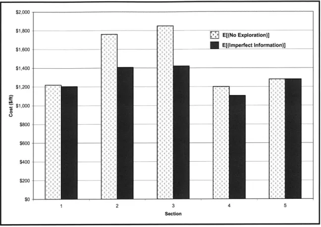
Figure 2.22: Expected Costs of "No Exploration" and "Imperfect Information" for 51

Application Example 2

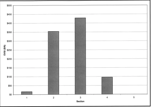
Figure 2.23: EVSI by Section for Application Example 2 52

Figure 3.1: Input Parameters 56

Figure 3.2: Decision Tree for No Exploration 57

Figure 3.3: Matrix Solution for the "No Exploration" Alternative 57

Figure 3.4: Decision Tree for "Imperfect Information" 59

Figure 3.5: Left-Most Branches of the Tree for the "Exploration" Alternative 60

Figure 3.6: Posterior Probabilities Matrix 60

Figure 3.7: Expected Costs of Strategies Matrix 61

Figure 3.8: Expected Cheapest Strategies 62

Figure 3.9: Probability Density Function of 64

Figure 3.10: Input Parameters for Example in Chapter 2 66

Figure 3.11: Main Menu 67

Figure 3.12: Input Parameter Definitions 68

Figure 3.13: Geologic State Descriptions 69

Figure 3.14: "Geologic and Cost Parameters" Pop-Up 70

Figure 3.15: Construction Strategies Considered 71

Figure 3.16: "Geologic and Cost Parameters" Pop-Up 72

Figure 3.17: Main Menu/Define Prior Probability Matrix 73

Figure 3.18: Prior Probability Matrix Values 74

Figure 3.19: Construction Cost Matrix 75

Figure 3.20: Reliability Matrix 76

(7)

Figure 3.22: Decision Tree for "No Exploration" 78

Figure 3.23: Decision tree for "Exploration" 79

Figure 3.24: Decision-Driving Outcomes 80

Figure 3.25: Probabilistic Analysis/Construction Cost Matrix 81

Figure 3.26: Main Menu/Probabilistic Analysis 82

Figure 3.27: EVSI Distribution and P[Exploration will not be Beneficial] 83

Figure 4.1: Aerial view of North Kenmore Tunnel 85

Figure 4.2: Geologic Profile for North Kenmore Tunnel 85

Figure 4.3 Expected Costs of Tunnel Section for No Exploration, Perfect and 94 Imperfect Exploration

Figure 4.4 EVPI and EVSI 94

Figure 4.5: EVSI and Cost of Exploration for North Kenmore Tunnel 95

Figure 4.6: Geologic Profile showing Location where Exploration is expected to 96

be beneficial

Figure 4.7: Decision Tree for "No Exploration" in Section 7 for North Kenmore 97

Tunnel

Figure 4.8: Probability Distribution of Expected Costs 98

Figure 4.9: Probability distribution for EVSI 98

Figure 4.10: Probability that Exploration will be beneficial for the Uniform and 99

(8)

LIST OF TABLES

Table 2.1: Deterministic Phase Characteristics for Tunnel Exploration 24 Table 2.2: Influence of Construction Strategy Costs on EVSI (for positive region) 32

Table 2.3: Sensitivity Results for Prior Probability Matrix 35

Table 2.4: Sensitivity Analysis Results for Reliability Matrix Entries 37

Table 4.1: Definition of Geologic States 86

Table 4.2: Prior Probability Matrix for North Kenmore Tunnel 87

Table 4.3: Exploration Reliability for North Kenmore Tunnel 88

Table 4.4: Construction Cost Matrix for North Kenmore Tunnel 88

Table 4.5: Expected Costs for Different Construction Methods in Different 90

Tunnel Sections

Table 4.6: Minimum Expected Costs, EVPI, and EVSI in the different Tunnel 91

(9)

CHAPTER 1 INTRODUCTION

Tunnels are subsurface passages which are often constructed without removing the overlying rock or soil (Szechy 1961). It follows that the lack of a priori knowledge of subsurface conditions poses major challenges in their preliminary design and planning. While the tunnel's general location is governed by existing needs, the exact location is often determined by the prevailing geologic conditions in the area. Initial reliable information on the geologic conditions is therefore vital for predicting the loads acting on the tunnel and the choice of construction method(s) to be employed. In the absence of such information, conservative designs and choices of construction methods (assuming worst geologic conditions) are often assumed. These conservative assumptions lead to inflated costs. Considerable construction savings may therefore be achieved through the proper collection and interpretation of initial reliable information on the existing geologic conditions.

In this initial planning phase of a tunnel project, information on the existing subsurface conditions is obtained from experts and geologists. Based on their experience, existing geologic maps, and their intuition, they may indicate with some certainty existing geologic formations, or geologic conditions that may render construction work difficult or sometimes even impossible. Consequently, the progress and construction costs of a tunneling project depend highly on the engineer's choice of construction strategies to suit the predicted subsurface conditions and on the reliability of the initial information obtained from experts. In addition, the linear nature of tunnels requires linear construction sequencing that highly restricts the flexibility to changes in construction

(10)

strategies. In fact, nearly any small variation in construction strategy may affect the progress and construction costs of a tunnelling project.

Construction strategies that are the best alternative for tunneling through a particular geologic state given cost, time, resource, plant, and material constraints, may prove to be unsuited in other states. The engineer thus faces the major challenge of matching construction strategies to the uncertain subsurface conditions. For a given geologic profile, the optimal choice of construction strategy/strategies depends on:

1. The extent of the geologic states in which each construction strategy is technically feasible.

2. The associated impact (cost and time) of employing each strategy/strategies in each geologic state.

3. The impact (cost and time) of changing from one construction strategy to

another.

Following the initial gathering of information and devising the corresponding construction strategy/strategies, the engineer must decide whether he feels confident enough to begin construction or whether gathering further information on the existing subsurface conditions would be more beneficial. Site exploration allows one to collect further information on the existing geologic states. However, exploration results provide information about the geologic states in the vicinity of the area being explored only; predictions about neighboring states have to be inferred subjectively by experts based on the exploration results. It should be noted that exploration results are not always indicative of the true nature of the existing subsurface conditions. Exploration results may therefore be uncertain in themselves. Moreover, exploration itself involves a cost. The aim of exploration planning is therefore to minimize total costs of construction plus

(11)

exploration. This cost constraint on exploration restricts the extent of desired exploration planning, boiling it down to a matter of maximizing the value of information obtained through exploration. Specifically, given initial information on the geologic states, exploration planning should determine:

1. Whether it would be beneficial to explore, and if so, 2. Where along the tunnel alignment should one explore.

1.1 PROBLEM STATEMENT/SCOPE

Present approaches to the tunnel exploration problem are mostly based on intuition, experience, and conservative assumptions that may lead to inconsistencies affecting decisions in the planning phase of a tunnel project. These assumptions may lead to decisions that result in inflated project costs on the one hand or underprediction cost and time on the other hand. Significant cost savings may be achieved through the application of decision theory to the tunnel exploration problem (Einstein et al 1978). Based on the model proposed by Einstein et al (1978), this thesis presents analytical and practical techniques for tunnel exploration planning; specifically, these techniques help in deciding:

1. Whether it would be beneficial to explore, and if so,

(12)

1.2 DEFINITIONS

The key terms that are used in the context of this thesis are defined in this section.

1.2.1 CONSTRUCTION STRATEGY

The term construction strategy in the context of this thesis refers not only to the excavation method and support procedure implemented, but includes also the type of equipment and the material used for the initial support.

1.2.2 GEOLOGIC STATE

Each geologic state represents a particular combination of geological parameters such as rock or soil type, jointing, foliation, gas, and groundwater conditions. Therefore, for a given geologic state, there can be more than one technically feasible construction strategy with some strategies being more conservative than others.

1.3 OUTLINE

Chapter 2 first reviews the decision analytical procedure for tunnel exploration as proposed by Einstein et al (1978) through two examples; one involving a single-section tunnel, and the other involving a multiple-section tunnel. In Chapter 3, numerical techniques for implementing the model in a programming package are outlined, and an application in Visual Basic for Applications that implements the model for a generic tunnel is described. The North Kenmore Tunnel will serve as a case study for the model in Chapter 4. Finally, Chapter 5 will highlight the major conclusions and provides recommendations for future work.

(13)

CHAPTER 2 DECISION ANALYSIS for TUNNEL EXPLORATION (DATE)

2.1 THE DECISION CYCLE

Figure 2.1 represents the decision-making process under uncertainty for engineering applications as proposed by Karam and Einstein (2005). In the deterministic phase, one selects the initial parameters and relates them to decision-driving outcomes through a model(s). Initial parameters are decision variables that can be controlled by the decision maker, and state variables representing the uncontrollable environment. The decision-driving outcomes may be related to one another through an objective function often involving cost or time criteria. Sensitivity analyses allow one to identify the most influential input variables; those variables with minimal influence can be left constant in the rest of the analyses.

In the probabilistic phase, uncertainties are incorporated into the analyses while maintaining the same relationships as in the deterministic phase. Decision-driving outcomes, such as cost, will then be in the form probability distributions. Decisions are made based on these outcomes. The decision on whether the collection of further information would be beneficial is done in the information phase (refer to Figure 2.1).

(14)

... ... UpdatinG ...---.. Probabilistic (Model) Phase

- Express probabilities and create probabilistic models

" Conduct probabilistic analyses

" Rank input parameters

Decision ... ... Information... Information (Model) Phase - Create information models

- Find expected values of information

- Conduct probabilistic sensitivity analyses

----.-.---...

Figure 2.1: The Decision Cycle

2.2 DECISION ANALYSIS for TUNNEL EXPLORATION

Exploration planning is a classic problem of decision making under uncertainty. The application of decision analysis to tunnel exploration is well established (Einstein et al,

1978) and will be described in the following sections through examples. First, an

example for a single-section tunnel is presented, followed by an example that extends the analysis to a multiple-section tunnel.

Collect Information

Deterministic (Model) Phase

- Select input parameters

" Relate input parameters to decision-driving outcomes

(15)

2.3 SINGLE-SECTION TUNNELS 2.3.1 DETERMINISTIC PHASE

The aim of exploration planning is to determine:

1. Whether it would be beneficial to explore, and if so,

2. Where along the tunnel alignment should one explore.

The model devised by Einstein et al (1978) will be demonstrated through an example. Consider a proposed single-section tunnel as shown in Figure 2.2. Based on their previous local experience, their intuition, and local geologic maps, geologists and engineers predict that the existing geologic states in this section can be either 1 G, 2G, or 3G. The model assumes that only one of these geologic states may actually exist in the

section. A: Start of B: End of Tunnel Tunnel 1G Tunnel Alignment .2 --- i_ _ __ _ __ _ _ L

1G Predicted Geologic State in Section I

Figure 2.2: Proposed Single Section Tunnel Alignment

Probability values are assigned to each of the geologic states (1G, 2G, and 3G) reflecting the likelihood of their existence in the section based on the geologists' and

(16)

engineers' assessment. These values can be organized in matrix form. This matrix will be referred to as the Prior Probability Matrix and is shown in Figure 2.3. The entries in the matrix are the probabilities that the true geologic state in the section is the one indicated by the matrix columns. Namely, P1G is the probability that the true geologic state is 1 G in the section; p2G is the probability that the true geologic state is 2G in the

section; and p3G is the probability that the true geologic state is 3G in the section. These probabilities are determined by the geologists'/engineers' assessment.

Note that the summation of P1G, p2G, and P3G must always equal 1 based on the assumption that none of the geologic states can coexist in the section.

True Geologic State

1G 2G 3G

Prior Probability Matrix = Section 1 [p1G P2G p3G] Figure 2.3: Prior Probability Matrix

Alternative construction strategies to suit each of the possible geologic states 1G, 2G,

and 3G given cost, time, resource, and material availability constraints are then considered. In this example, three construction strategies denoted by S1, S2, and S3

are considered. The construction costs of employing each of these strategies (S1, S2, and S3) in each of the geologic states (1G, 2G, and 3G) can also be represented in

matrix form. This matrix will be referred to as the Construction Cost Matrix and is shown in Figure 2.4. The entries in the matrix are the construction costs of employing each of the considered strategies (matrix rows) in each of the geologic states (matrix columns).

(17)

True Geologic State

1G 2G 3G

S1 CS1,1G CS1,2G CS1,3G

Construction Cost Matrix = Construction Strategy S2 CS2,1G CS2,2G CS2,3G

S3 [CS3,1G CS3,2G _{CS3,3G_}

Figure 2.4: Construction Cost Matrix

The exploration reliability is represented in matrix form as well. This matrix will be referred to as the Reliability Matrix and is shown in Figure 2.5. The probability values in the matrix are the result of subjective assessment of the performance of the exploration method in the geologic states. For example, P2G,1G is the probability that the chosen exploration method indicates 2G given that the true geologic state is 1 G.

Exploration Method Indicates

1G 2G 3G

1G P1G,1G P2G,1G P3G,1G

Reliability Matrix = True State 2G P1G,2G P2G,2G P3G,2G

3G [PG,3G P2G,3G P3G,3G_

Figure 2.5: Reliability Matrix Note that the rows in the Reliability Matrix have to add up to 1.

The Prior Probability Matrix, the Construction Cost Matrix, and the Reliability Matrix are the input parameters for the model through which decisions are made.

In essence, one is faced with two alternatives when deciding on whether to explore: 1. Explore and use the information obtained from exploration before proceeding with construction (from now on referred to as the "Imperfect Information" alternative) and 2. Proceed with construction without exploring (from now on referred to as the "No Exploration" alternative). To decide between these two alternatives, one has to compare the expected benefits of exploring and compare them to the expected benefits of not

(18)

exploring. If exploring provides information on the geologic conditions that ultimately leads to a reduction in the total expected costs plus the cost of exploration (when compared to the expected cost of "No Exploration"), then exploring is beneficial. If on the other hand exploring provides information on the geologic conditions that doesn't ultimately reduce the expected total costs plus the cost of exploration (when compared to the expected costs of "No Exploration") then exploring is not beneficial losing the cost of exploration in the process.

Quantitatively, the value of information obtained through exploration is evaluated by finding the difference between the expected costs of the "No Exploration" alternative and the expected costs of exploring (denoted by the "Imperfect Information" alternative). This difference is known as the Expected Value of Sample Information (EVSI) and is

defined in Equation 2.1.

Equation 2.1

Expected Value of Sample _ Expected Cost of _ Expected Cost of Information (EVSI) - "No Exploration" "Imperfect Information"

If the EVSI is positive then one is expected to save the value of the EVSI by exploring.

However, since exploration comes with a cost as well the expected amount saved is actually the difference between the EVSI and the cost of exploration. If, on the other hand, the EVSI is less than the cost of exploration then one is expected to lose the difference between the EVSI and the cost of exploration as a result of exploring. In this case exploration is not beneficial.

(19)

Decision tree analysis is used to calculate the expected costs of not exploring ("No Exploration" alternative) and the expected costs of exploring ("Imperfect Information" alternative). For the preceding example, Figure 2.6 shows the decision tree for the "No Exploration" alternative.

Figure 2.6: Decision Tree for "No Exploration"

In this example, one has the choice between three construction strategies: S1, S2, and S3. If one chooses to employ S1, then there is a P1G (obtained from the Prior Probability

Matrix) chance of encountering geologic state 1 G, a P2G chance of encountering geologic state 2G, and a P3G chance of encountering geologic state 3G. In the case that one chooses to employ S1 and encounters the geologic state 1G, the corresponding

E["No Exploration"] = Min(E[Cost S1]), E[Cost S2], E[Cost S3])

Cost of S1 in 1G = CSlIG Cost of S in 2G = CS1,2G Cost of S1 in 3G = CS1,3G Cost of S2 in IG = CS2,IG Cost of S2 in 2G = CS2,2G Cost of S2 in 3G = CS2,3G Cost of S3 in 1G = CS3,IG Cost of S3 in 2G = CS3,2G Cost of S3 in 3G = CS3,3G P[1G] =P1G E[Cost S1] PI S-1 [3G] =p3G P[1G] =P1G E[Cost S2] P[G I S-2 P2]=p2G 0-% P[322G] =P3G E[Cost S3] P[1G] =p1G P[2G] =p2G P[3G] =p3G E[Cost S3]

**=P1GCS3,1G+P2GCS3,2G+P3G*CS3,3G**

(20)

construction cost is given by CS1,1G (obtained from the Construction Cost Matrix). In the case that one chooses to employ S1 and encounters geologic state 2G, the corresponding cost is given by CS1,2G, and so on. The expected cost of employing S1 is then given by Equation 2.2:

Equation 2.2

E[Cost S1] = PIG * CS1,1G +P 2G *CS1,2G + P3G * CS1,3G

The expected costs of employing strategies S2 and S3 can be calculated in a similar manner. These expected costs are evaluated as shown in Figure 2.6. The expected cost of "No Exploration" is then the minimum of E[Cost SI], E[Cost S2], and E[Cost S3].

By identifying the minimum expected construction costs, the corresponding strategy is

the least costly in the section and is likely to be employed based on the available information prior to exploration.

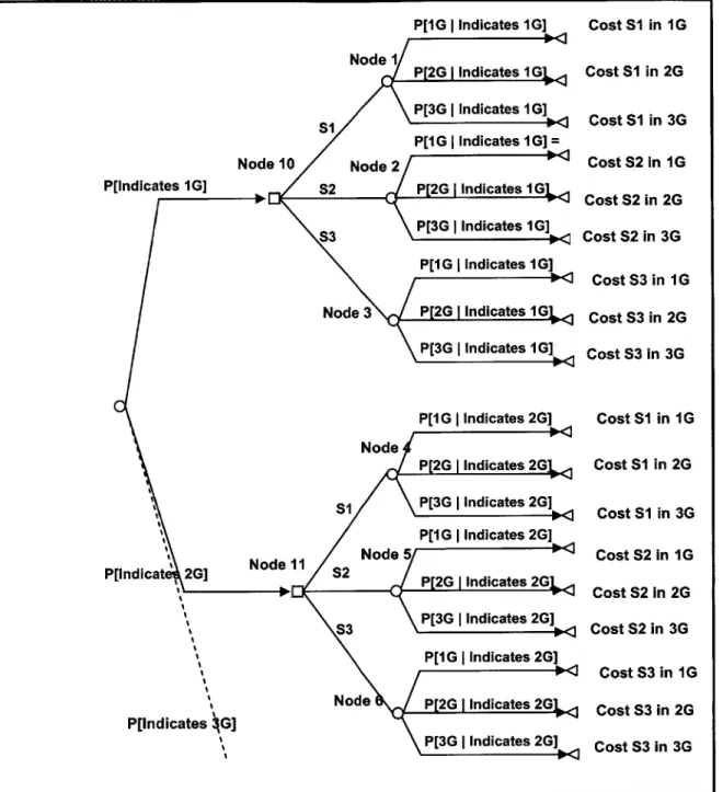
The tree for the "Imperfect Information" alternative is shown in Figure 2.7. In this case, one makes decisions based on the exploration results. The exploration results will indicate the existence of either one of the three geologic states in the section. They will either indicate that geologic state 1 G, or that geologic state 2G, or that geologic state 3G exists in the section (based on the assumption that no two geologic states can coexist in a given section). The probability that the exploration results indicate any one of the three geologic states is obtained from the Total Probability Theorem. Equation 2.3 shows this for the exploration results indicating 1 G:

Equation 2.3

P[Indicates 1 G] = P[lndicates 1 G 11 G] * P[I G] + P[Indicates 1 G |2G]* P[2G] +

P[Indicates 1 G |3G] * P[3G]

P[lndicates 1G|1G] is the probability that the exploration results indicate 1G given that the actual geologic state is 1G, and P[lndicates 1G|2G] is the probability that the

(21)

exploration results indicate 1G given that the actual geologic is 2G, etc. These values are obtained from the Reliability Matrix (Figure 2.5). For example, P[Indicates 1Gl1G]

corresponds to P1G,1G in the Reliability Matrix, and P[Indicates 1G|2G] corresponds to P1G,2G in the reliability matrix etc. The probability that the exploration results indicate 2G

(22)

r-Lu C11

C12

uSL 0 Ij = P[1G I Indicates 1G]

'[1G Ind IG]]+C12P[2G I Indicates 1G]+ n G

P[3G | Indicates 1G] Node 1 P[2G I Indicates 1G = P[3G | Indicates 1G] P[1G I Indicates IG] = P[Indicates 1G] S2 P[2G I Indicates 2G = Node 2 P[3G | Indicates 1G] = S3 P[1G | Indicates 1G] = No < P[2G _I_{Indicates 2G} =G P[3G I Indicates 2G] = P[1G I Indicates 2G] = 10 < P[2G | Indicates 2G]L= S1 P[3G I Indicates 2G]= P[1G IIndicates 2G] = 10 < P[Indicate 2G] _S2 _{P[2G I}_Indicates_2G1= P[3G|IIndicates 2G] = S3 ₀. P[1G I Indicates 2G] = P[2G I Indicates _{2G ;=-<} P[3G | Indicates 2G] = E[Cost "Imperfect Information"] =

P[Indicates 1G]*(Min(E[Cost SI], E[Cost S2], E[Cost S3])+P[Indicates 2G]Min(E[Co E[Cost S2], E[Cost S3]) Cost S1 in 1G = C11 Cost S1 in 2G = C12 Cost S1 in 3G = C13 Cost S2 in 1G = C21 Cost S2 in 2G = C22 Cost S2 in 3G = C2 3 Cost S3 in 1G = C31 Cost S3 in 2G = C32 Cost S3 in 3G = C33 Cost S1 in 1G = C₁₁ Cost S1 in 2G = C12 Cost S1 in 3G = C13 Cost S2 in 1G = C21 Cost S2 in 2G = C₂₂ Cost S2 in 3G = C23 Cost S3 in 1G = C₃₁ Cost S3 in 2G = C32 Cost S3 in 3G = C33 t S1],

Figure 2.7: Decision Tree for "Imperfect Information"

The probabilities at the end of the tree are known as the posterior probabilities. These posterior probabilities are calculated using Bayes' theorem as shown in Equation 2.4

(23)

(where i represents the true geologic state, and

j

represents the geologic state indicated

by the exploration results):

Equation 2.4:

P[iG I Exploration Indicates jG] = P[Exploration Indicates jG I iG]P[iG] Reliability Matrix P[Exploration Indicates jG] Total Probability

These are the probabilities of actually finding each of the geologic states in the section given that the exploration results indicate the presence of a geologic state. Solving the tree is then analogous to that for "No Exploration," as shown in Figure 2.7. Finally the expected cost of "Imperfect Information" is calculated as follows:

Equation 2.5 E[Cost "Imperfect Information"] =

P[lndicates 1G]*Min(E[Cost S1],E[Cost S21,E[Cost S3])+P[Indicates 2G]*Min(E[Cost S1], E[Cost S2], E[Cost S3]) +P[lndicates 3G]*Min(E[Cost S1], E[Cost S2], E[Cost S3])

The EVSI (Equation 2.1) can then be used to determine whether exploration is beneficial. If the EVSI is greater than the cost of exploration then exploring is expected to be beneficial with expected savings equal to the difference between the EVSI and the cost of exploration. If on the other hand the EVSI is less than the cost of exploration then exploring is not expected to be beneficial with expected losses equaling the difference between the EVSI and the cost of exploration.

Table 2.1 summarizes the aspects of the deterministic phase for the tunnel exploration problem.

(24)

Table 2.1: Deterministic Phase Characteristics for Tunnel Exploration

Decision Problem Determine:

1. If exploration is beneficial, and if so,

2. Where along the tunnel alignment should one explore

Alternatives 1. Explore

2. Don't Explore

Outcomes 1. Expected Value of Sample

Information (EVSI)

Decision Input Variables 1. Exploration Cost

2. Prior Probabilities

3. Exploration Reliability

4. Construction Strategy Costs

5. Geologic States

Relationship between Variables Decision Tree Analysis

Value of Outcomes Expected Costs

Source: Einstein et al (1978)

In the next section, a numerical example for a single section tunnel is presented.

2.3.2 APPLICATION EXAMPLE 1 (SINGLE SECTION TUNNEL)

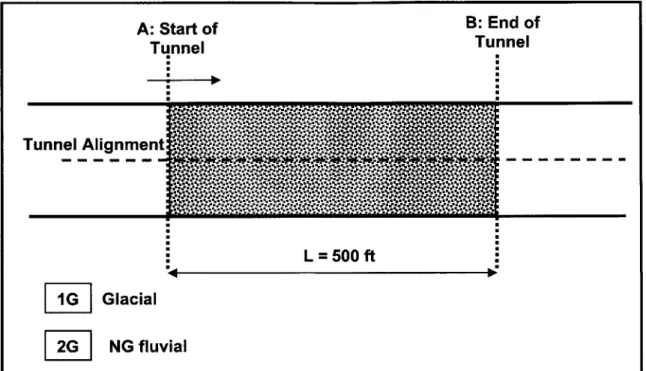
Consider the proposed single section tunnel alignment of length 500 ft depicted in Figure

(25)

A: Start of B: End of Tunnel Tunnel Tunnel Alignment L = 500 ft 1G Glacial

W

NG fluvial

Figure 2.8: Proposed Single Section Tunnel Alignment

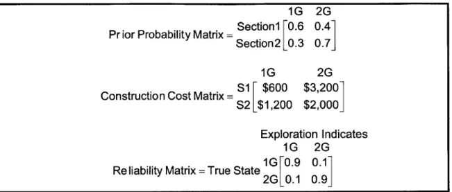
Geologists'/engineers' assessments indicate that there is a probability of 0.6 that the true geologic state in the section is 1 G, and therefore a probability of 0.4 that the true

geologic state in the section is 2G. This is summarized in the Prior Probability Matrix shown in Figure 2.9. The two considered construction strategies for this tunnel are: 1. SI: Slurry Shield, and 2. S2: EPB machine. The costs (per ft) of employing S1 and S2 in

geologic states 1G and 2G are summarized in the Construction Cost Matrix shown in Figure 2.9. The reliability of the exploration method used is also summarized in Figure

(26)

1G 2G

Pr ior Probability Matrix = [0.6 0.4]

1G 2G

Construction Cost Matrix = Slurry Shield $600 $3,200

EPB [$1,200 $2,000] Exploration Indicates

1G 2G

Reliability Matrix = True State IG[0.9

0.11

2G 0.1 0.9

Figure 2.9: Prior Probability, Construction Cost, and Reliability Matrices

The decision tree for "No Exploration" is shown in Figure 2.10. Prior to exploration, the expected cost of employing strategy S1 is $1,640/ft and the expected cost of using strategy S2 is $1,520/ft in the section (calculations are shown in Figure 2.10). One therefore decides to use the cheaper strategy S2 since S2 is expected to be $120/ft cheaper than using strategy S1 in the section.

E[Cost S1] = 0.6*600 + 0.4*3,200

=$1,640/ft P[1G] 0.6 $600

E[Cost "No Exploration"]=

_S1

Min(E[Cost S1], E[Cost S2]) $3,200 = $1,520/ft P[IG] = 0.6 $1,200 S2 E[Cost S2] = 0.6*1,200 + 0.4*2,000 ...-- P[2G] = 0.4 $2,000 = $1,520/ft

Figure 2.10: Decision Tree for "No Exploration" (Application Example 1)

(27)

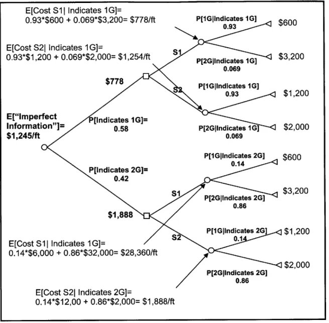
E[Cost S1 I Indicates 1 G]= 0.93*$600 + 0.069*$3,200= $778/ft P[lGjIndicates _0.93 1G] $600 E[Cost S21 Indicates 1G]= 0.93*$1,200 + 0.069*$2,000= $1,254/ft P[2Glindicates 1G] $3,200 0.069 $778 _{P[1G|Indicates 1G]} 0.93 $1,200

E["Imperfect _{[Indicates IG]=}

Information"]= 0.58 P[2GIndicates IG] $2,000

$1,245/ft 0.069 P[1GlIndicates 2G] $600 P[lndicates 2G]= 0.14 0.42 S1 P[2GlIndicates 2G] $3,200 0.86 $1, 888 P[1Glindicates 2G] $1,200 E[Cost S11 Indicates 1G]= S 01 0.14*$6,000 + 0.86*$32,000= $28,360/ft $2,000 P[2GIlndicates 2G] 0.86 E[Cost S21 Indicates 2G]= 0.14*$12,00 + 0.86*$2,000= $1,888/ft

Figure 2.11: Decision Tree for "Imperfect Information" (Application Example 1)

The probability that exploration indicates 1G or 2G can be calculated using the Total Probability Theorem as follows:

P[Indicates 1 G] = P[Indicates 1 G 11 G] * P[1 G] + P[Indicates 1 G I 2G] * P[2G] = 0.9 * 0.6 + 0.1* 0.4 = 0.58

(28)

P[Indicates 2G] = P[Indicates 2G I1G] * P[1G]+ P[Indicates 2G 12G] * P[2G] = 0.1* 0.6 + 0.9 * 0.4

= 0.42

Posterior probabilities (probabilities of encountering the true geologic state given that the exploration results indicate the same or another geologic state) are calculated using Bayes' Theorem as follows:

P[1GIndicates 1 G] = P[Indicates 1G|1G] * P[1G] 0.9 * 0.6 P[Indicates 1 G] 0.58 = 0.93 P[2G|Indicates 1G] = P[Indicates 1 G 12G] * P[2G] 0.1 * 0.4 P[lndicates 1 G] 0.58 = 0.069

(Note: as a check these two values have to add up to one).

P[1G|Indicates 2G] =P[Indicates 2Gl1G]*P[1G] 0.1*0.6 P[Indicates 2G] 0.42 =0.14 P[2G Indicates 2G] =P[Indicates 2G

I

2G] * P[2G] 0.9 * 0.4 P[lndicates 2G] 0.42 = 0.86

(Note: as a check these two values have to add up to one).

The decision tree is then solved in an analogous manner to the "No Exploration" alternative. The expected cost of "Imperfect Information" is $1,245/ft.

Recalling that the EVSI for the section is given by,

Expected Value of Sample _ Expected Cost of - Expected Cost of

Information (EVS)~ "No Exploration" "Imperfect Information" the EVSI for this single section tunnel is then:

(29)

Prior to including the cost of exploration, it follows that as a result of exploring further the total expected savings for the 500 ft single section tunnel would be $137,500

(500ft*$275/ft). Assume that the cost of exploration amounts to $100,000. The savings

would then be $37,500 (Total Savings due to Exploration - Cost of Exploration). Based on this initial deterministic analysis exploration is expected to be beneficial in this

section.

SENSITIVITY ANALYSES

Sensitivity analyses allow one to determine the influence of the input parameters on the

EVSI and therefore on the decisions of whether exploration will be beneficial and of the

optimal location of exploration along the tunnel's alignment. The parameters that do not have much influence can then be left constant for the rest of the analyses.

CONSTRUCTION COST MATRIX

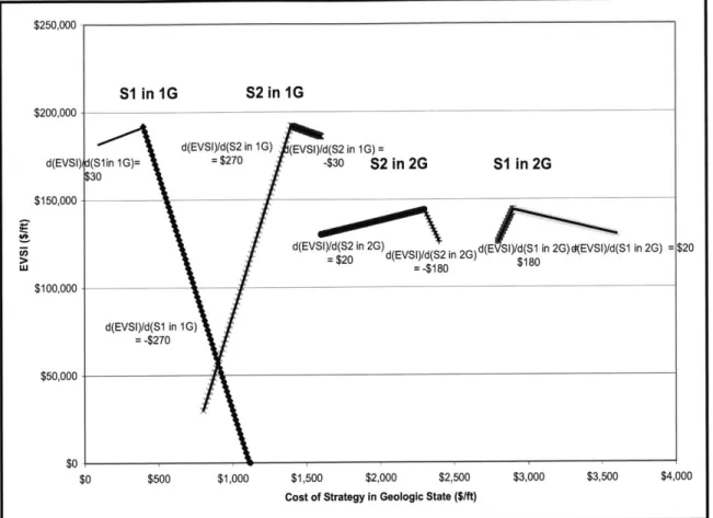
Consider the Construction Cost Matrix in Figure 2.9. The construction costs for the two construction strategies (S-1 and S-2) in the different geologic states (1 G and 2G) are varied independently, and so sensitivity analyses on each parameter is performed while holding the others constant. This is a one parameter sensitivity analysis, as all other input parameters are held constant. The results are shown in Figure 2.12.

(30)

$250,000 SI in IG S2 in 1G $200,000-d(EVSI)/d(S2 in 1G) (EVSI)/d(S2 in 1 G)= d(EVSI)d(Slin 1G)= $270 -$30 S2 in 2G SI in 2G $30 $150,000

d(EVSI)/d(S2 in 2G) i n 2G) d(En VSId(S1 in 2G) = $20

d(VI)/d(S2 n2~( $100,000 d(EVSI)/d(S1 in 1G) $50,000 -$0 $0 $500 $1,000 $1,500 $2,000 $2,500 $3,000 $3,500 $4,000

Cost of Strategy in Geologic State ($/ft)

Figure 2.12: Sensitivity of EVSI to Construction Costs per Unit Length (Application

Example 1)

As seen in Figure 2.12, the influence of varying the construction costs within a particular geologic state on the EVSI can be characterized by curves with these three properties:

1. A singular point at which the slope changes abruptly from being positive

to negative.

2. For construction costs lower than those corresponding to the singular points, an increase in construction costs per unit length results in an

increase in the EVSI (positive slope).

3. For construction costs per unit length higher than those corresponding to

the singular point, an increase in construction costs per unit length results in a decrease in the EVSI (negative slope).

(31)

Consider, for example, the entry S2 in 1 G of the Construction Cost Matrix ($1,200).

1G 2G

Construction Cost Matrix=SI[$600 $3,200] S2 $1,200 $2,000

The construction cost of S2 in 1G is varied linearly between $800 and $1600 (keeping all the other entries constant). The singular point corresponds to a cost of $1,400 (as can be seen in Figure 2.12). For construction costs below this value, an increase of one dollar in construction costs yields an increase of $270 in the EVSI. For construction costs above this value, an increase of one dollar in construction costs yields a decrease of $30 in the EVSI. This abrupt change occurs because of switching of construction strategies. For values below that corresponding to the singular point ($1,400), employing strategy S2 is cheaper than employing strategy S1 in geologic state 1-G. As the construction cost values for S2 in 1 G are increased exploration becomes

increasingly beneficial (reflected in an increasing EVSI) because the construction costs of employing S2 becomes comparable to employing strategy S1 in the section. Increasing the costs of S2 in 1G beyond that corresponding to the singular point ($1,400) makes exploration decreasingly important (decreasing EVSI) because it becomes increasingly apparent that S1 in 1G is cheaper than S2 in 1G. At the singular point, the "switch" between S2 and S1 occurs, and the sensitivity analysis on construction costs beyond this point actually corresponds to the influence of S1 in 1G

(as opposed to the intended S2 in 1G) on the EVSI as indicated by the slopes in Figure 2.12:

d(EVSI) _{(less than its singular point)}.d(EVSI) ₌ _- _{(greater than singular its point)}

(32)

In other words, beyond the cost corresponding to the singular point of S2 in 1G the influence of the cost of S1 in 1G on the EVSI is being examined. The same can be said about S1 and S2 in 2G (see Figure 2.12).

The magnitude of the positive slopes of the lines determines which construction strategy costs have the most influence on the EVSI. In the example, the ranking of the influence of the strategy costs in the geologic states on the EVSI is summarized in Table 2.2 (with

1 corresponding to the most influential).

Table 2.2: Influence of Construction Strategy Costs on EVSI (for positive region)

1. S2 in 1G d(EVSI)/d(S2 in 1G) = $270

2. S1 in 2G d(EVSI)/d(S1 in 2G) = $180 3. S1 in 1G d(EVSI)/d(S2 in 1G) = $30

4. S2 in 2G d(EVSI)/d(S2 in 1G) = $20

CONSTRUCTION COST SENSITIVITY ANALYSIS CONCLUSIONS

The above analysis yields the following conclusions:

1) The construction cost of S2 in 1G has the largest influence on the EVSI: a one dollar change in the cost of S2 in 1G yields a $270 change in the EVSI.

2) The construction costs of S1 in 1G and S2 in 2G have a minimal effect on the

EVSI and will therefore be left constant throughout the rest of the analysis.

3) When conducting sensitivity analyses on the construction costs, only the

(33)

4) The maximum possible EVSI is reached when all entries in the Construction Cost Matrix are equal to the values that correspond to their singular points. The EVSI is greatest when all the entries assume these values and exploration is therefore most beneficial at this point.

PRIOR PROBABILITY MATRIX

Performing sensitivity analysis on the prior probability matrix is not straightforward in that one cannot simply vary one (or more) probability entries of these matrices. This is because the probabilities are not independent. The sum of the probabilities in each row of the Prior Probability Matrix must equal to one because these events are mutually exclusive and collectively exhaustive. Therefore, when performing sensitivity analyses and one parameter is varied, e.g. P1G, we need to ensure that the second dependent

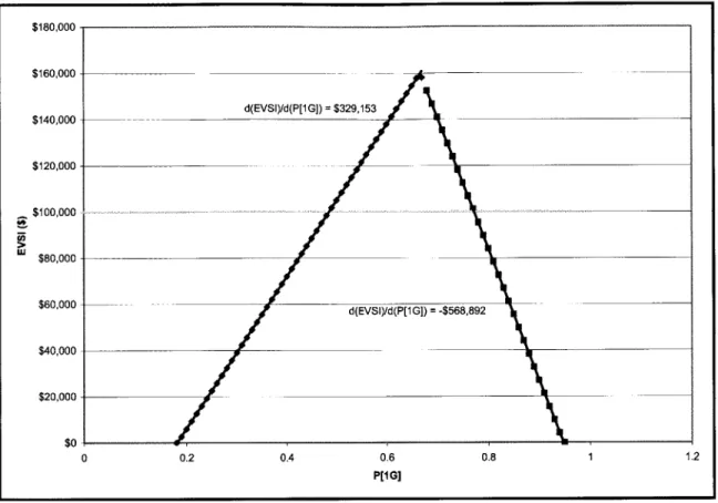
parameter, P2G in this example, is varied as well. The results of sensitivity analyses for

the P1G entry in the Prior Probability Matrix shown in Figure 2.9 are shown in Figure

(34)

$180,000 $160,000 d(EVSI)/d(P[1G]) = $329,153 $140,000 $120,000-$100,000 .... .= $80,000 $60,000 _{d(EVSI)/d(P[1G])}₌_-$568,892 $40,000 -$20,000 $0 0 0.2 0.4 0.6 0.8 1 1.2 P[1G]

Figure 2.13: Sensitivity of EVSI to PIG (Application Example 1)

Since the geologic states 1G and 2G cannot coexist in the section one is almost certain that geologic state 2G exists in the section when PIG is close to zero, and therefore exploration is not beneficial (reflected in the small EVSI value). At this point, construction strategy S2 is the cheaper strategy. As PIG is increased, one becomes increasingly uncertain about whether geologic state 1 G or geologic state 2G exists in the

section and therefore exploration is beneficial for this determination (reflected in the increasing EVSI). A singular point is reached when one is approximately 70% certain that geologic state 1G exists in the section. The switching event described in the previous section occurs again at this point. Beyond this singular point construction strategy S1 becomes the cheaper strategy. There are therefore two distinct regions in which sensitivity analysis should be conducted: 1. Probabilities below that corresponding

(35)

to the singular point, and 2. Probabilities above that corresponding to the singular point. These values are summarized in Table 2.3:

Table 2.3: Sensitivity Results for Prior Probability Matrix

P1G< 0.7 $329,153

0.7<P1G<1 $568,892

PRIOR PROBABILITIES SENSITIVITY ANALYSIS CONCLUSIONS

1) A 0.1 change in the prior probability values yields a change of $32,915.3 in the EVSI when P1G < 0.7.

2) A 0.1 change in the prior probability values yields a change of $56,889.2 in the

EVSI when 0.7 < P1G

<1-3) When conducting sensitivity analysis on the entries in the Prior Probability Matrix,

the singular point must be determined and the analysis be conducted in the regions below and above the singular point independently.

4) The EVSI takes on its maximum possible value when P1G is approximately 70% (at the singular point). Exploration is most beneficial at this value.

RELIABILITY MATRIX

Four scenarios were considered in the sensitivity analysis for the Reliability Matrix entries: 1. Varying P[lGllndicates 1G] between 0.5 to 1 (completely unreliable to completely reliable) when P[2G|Indicates 2G] = 1 (completely reliable), 2. Varying P[2GIlndicates 2G] between 0.5 to 1 when P[lGllndicates 1G] = 1, 3. Varying

(36)

P[lGllndicates 1G] between 0.5 to 1 when P[2G|Indicates 2G] = 0.5 (completely unreliable), 4. 2. Varying P[2G|Indicates 2G] between 0.5 to 1 when P[lGjlndicates 1G]

= 0.5. The results are summarized in Figure 2.14.

$200,000 $180,000 $160,000 _{d(EVSI)/d(P[Ind 1G|1G]} $180,000 $140,000 $120,000 - PA GI G] for. P[lnd 2G12G1 = 1 d(EVSI)/d(P(Ind 2G12G) $100,000--$4,0 d(EVSI)/d(P[Ind 2G12G]) LU _$240,00 $80,000 $60,000 G forrPnd2Gd2G]

Ptlfld IGIIGI =1 P[Ind 2G12G] for

$4,000- Ptlfld IGIIG) 0. d(EVSI)/d(P[Ind 1GI1G] = $180,00 $20,000 _{Pind 111Gj}_tor $0 P[Ind 2G12G] = 0.5 0.5 0.55 0.6 0.65 0.7 0.75 0.8 0.85 0.9 0.95 1 Probability Value

Figure 2.14: Sensitivity Analysis for Exploration Reliability (Application Example 1)

Note that the influence of the entries on the EVSI are independent of one another, reflected by the fact that P[Ind 1G|1G] has the same slope no matter what value P[lnd

2G12G] takes (except for the region when they are both very unreliable 0.5-0.66 in which

case exploration is clearly not beneficial reflected by the small EVSI values). Table 2.4 summarizes the results of the sensitivity analysis:

(37)

Table 2.4: Sensitivity Analysis Results for Reliability Matrix Entries

P[Indicates 2G12G] $240,000

P[Indicates 1GilG] $180,000

EXPLORATION RELIABILITY SENSITIVITY ANALYSIS CONCLUSIONS

1) A 0.1 change in the Reliability Matrix entries yields a change of $24,000 for

P[lndicates 2G12G] and a change of $18,000 for P[lndicates 1GilG].

2) The effects of entries indicating a geologic state on the EVSl are independent of the entries indicating other geologic states in the matrix.

3) When one entry is reliable and the other is completely unreliable(P[lnd iGjG] =

0.5), exploration may still be beneficial (see Figure 2.14).

4) When both entries are unreliable (0.5 - 0.66 in this case) exploration is never beneficial.

5) Exploration is most beneficial when the exploration results are completely

reliable.

GENERAL CONCLUSIONS FOR SENSITIVITY ANALYSES

The following general remarks can be concluded based on the sensitivity analysis for this example:

1) The entries in the Prior Probability Matrix seem to have the most influence on the EVSI (for small uncertainties in the Construction Cost Matrix).

2) The entries in the Reliability Matrix seem to have a significant influence on the

EVSI.

(38)

3) The collection of further information should be concentrated on information

leading to a better prediction of the subsurface geologic states.

4) Exploration is most beneficial when the EVSI is a maximum. The maximum possible value of EVSI occurs when the entries in the Construction Cost Matrix correspond to those indicated by their singular points, and the entries in the Prior Probability Matrix correspond to those indicated by their singular point, and when the exploration methods used are completely reliable. Intuitively, these findings make sense.

2.3.3 PROBABILISTIC PHASE

Uncertainty in the input variables is introduced in the Probabilistic Phase. The entries in the Prior Probability Matrix, the Construction Cost Matrix, and the Reliability Matrix are now assumed to be random variables with assigned probability distributions characterized by their respective parameters (mean, variance, etc.). The decision-tree model relating the input variables to the decision-driving outcomes derived in the Deterministic Phase remains the same for the Probabilistic Phase. Outcomes in the Probabilistic Phase are therefore in the form of probability distributions.

In practice, Monte Carlo techniques can be used to simulate the generation of probabilistic distributions and relate them to outcomes through a model.

The EVSI for each tunnel section then becomes a function of random variables that can be approximated by a normal distribution characterized by a mean and standard deviation (as per the Central Limit Theorem). In the deterministic phase, prior to considering uncertainties in the input parameters, exploration in a given section was deemed beneficial if the EVSI was greater than the cost of exploration in that section.

(39)

After the incorporation of uncertainty in the input parameters simulation may yield values of EVSI that are less than the cost of exploration and other values of EVSI that are greater than the cost of exploration in the same section, as shown in Figure 2.15. The decision-maker may not want to accept the assertion that exploration is beneficial unless and until simulation provides strong support for this assertion. Probabilities indicating the likelihood of exploration being beneficial can be determined by the area under the

normal curve as shown in Figure 2.15.

EVSI for Section 1

Cost of Exploration

--i P[No Exploration --- -~-- P[Exploration is is Beneficial] -Beneficial]

EVSI

Figure 2.15: EVSI for Section

It is then up to the decision-maker to determine the desired level-of confidence before taking the decision to explore depending on his risk-attitude. EVSI of a particular section is assumed to be a normal distribution with a known mean and variance, that is to say EVSI ~ N(X, 02). The Z-statistic is used to measure the distance between the mean value of the EVSI and the cost of exploration. This is given in Equation 2.6:

(40)

Equation 2.6

Z =X-o S

X - Mean of EVSI distribution (obtained through simulation) po - Cost of Exploration

S - Standard deviation of EVSI distribution (obtained through simulation)

The standardized variable Z reflects the distance between X and po in "standard deviations units." Larger positive values of Z (small S or/and large (X - po)) indicate that exploration is beneficial. The decision-maker could then specify the level of Z at which he feels confident enough that exploration would be beneficial.

2.3.3.1 POSSIBLE DECISION ERRORS AND THEIR CONSEQUENCES

Choosing confidence levels by which the decision-maker feels confident that exploration would be beneficial (or not) depends on an understanding of the errors and their consequences that he may inadvertently face when taking certain decisions. There are in essence two main possible types of errors in exploration planning. The first type of error occurs when the decision-maker decides to explore when in reality he was better off not exploring at all; while the second type of error occurs when the decision-maker decides not to explore when in reality he was better off exploring. If through exploration, the expected construction costs are not less than those expected prior to exploration then exploring further was unnecessary.

Consider for example a 2-section tunnel with 2 possible alternative construction strategies: 1. S1, and 2. S2. Prior to exploration, employing S1 in the first section followed by S2 in the second section is expected to yield the cheapest construction costs. Assume further that exploration is most beneficial in section 2. There are now 2 scenarios that could occur after exploring in section 2:

(41)

1) Exploration shows that employing S1 in section 1 followed by S2 in section 2 is the expected cheapest strategy (same as "No Exploration" alternative). 2) Exploration shows that employing S1 in section 1 followed by S1 in section

2 is the expected cheapest strategy (different from the "No Exploration" alternative).

In the first scenario, exploration did not lead to a reduction in the construction costs when compared to the "No Exploration" alternative, and the decision-maker was in retrospect better off not exploring at all. In fact, by exploring, the decision-maker lost the cost of exploration in the process. In the second scenario, exploration is expected to save the cost of switching from strategy S2 to strategy S1, because if one does not explore, one would eventually realize that employing S1 is cheaper than S2 in section 2 and may switch to S1 then.

Another type of error lies in the reliability of the exploration methods used. Consider the second scenario in which exploration showed that employing S1 in section 1 followed by

S1 in section 2 is the cheaper strategy. Since the exploration methods employed are not completely reliable, in reality, employing S1 in section 1 followed by S2 in section 2 may still be the cheapest strategy even after exploring. In this case, the decision to explore would yield expected losses that amount to the cost of exploration plus the cost of switching from construction strategy S1 to construction strategy S2. These risks are inherent in the problem and alleviating them is practically impossible. However, they can be assessed through probabilistic analyses. In the next section probabilistic analysis will be applied to Application Example 1.

(42)

2.3.4 APPLICATION EXAMPLE 1 (REVISITED)

Application example 1 assumed the values depicted in Figure 2.16 for the Prior Probability Matrix, the Construction Cost Matrix, and the Reliability Matrix. The EVSI was determined to be $137,500 and therefore exploration was beneficial and expected to yield an expected savings of $37,500 ($137,500 - Cost of Exploration = $100,000)

after considering the cost of exploration.

1G 2G

Prior Probability Matrix = [0.6 0.4]

1G 2G

EPB Machine

F$600

$3,200]

Construction Cost Matrix = I

EPB Machine with Dewatering L$1_,2 0 0 _$2,000]

Exploration Indicates

1G 2G

Reliability Matrix = True State IG[p.9

0.11

2G [0.1 0.9]

Figure 2.16: Input Parameters for Application Example I

One way to incorporate uncertainty on subjectively assigned probabilities is to specify a range of possible values, and assume a uniform distribution. Let X be a random variable that takes values between a and b according to a uniform distribution: X - U(a,b). The

probability density function of X is given by:

Equation 2.7 a<X<b

fX(x)= (b-a)

0; everywhere else

(43)

Equation 2.8

x-a _{; a<X<b} FX(x)= (b-a)

10; everywhere else

Figure 2.17(a) shows the probability density function of X and Figure 2.17(b) shows the cumulative distribution function of X.

fx(x) FX(x) AL

1

.---(b - a)

a (a+b) b X a b X

2

Figure 2.17(a) Probability Density Function of Figure 2.17(b) Cumulative Distribution

X Function of X

The expected value and variance of X are given by Equation 2.9:

Equation 2.9

E[X] = (a+ b)

2

Var[X] = 1 (b - a)2

12

INPUT PARAMETERS HAVING UNIFORM DISTRIBUTIONS

The effects on the EVSI of varying the input parameters according to uniform distributions are first considered. As a first step, probabilistic analysis is run on all three of the input parameters simultaneously. If the corresponding EVSI distribution clearly indicates that exploration is beneficial (or not) then further analysis of the individual input

(44)

parameters is not necessary. On the other hand, if the resulting EVSI distribution indicates an indecisive decision as to whether exploration is beneficial in the section, then each of the input parameters should be analyzed separately to determine which one has the most influence on the EVSI values.

A 20% error in the initial cost estimates is assumed. Consequently, each element in the

Construction Cost matrix is a uniformly distributed random variable with a minimum value that is 20% less than the value estimated in the deterministic phase and a maximum value that is 20% more than the value estimated in the deterministic phase. This is summarized in Equation 2.10:

Equation 2.10:

Cost of S1 in 1G- U($480,$720)

Cost of S1 in 2G - U($2,560,$3,840)

Cost of S2 in 1 G - U($960,$1,440)

Cost of S2 in 2G - U($1,600,$2,400)

The exploration method employed was assumed to be correct with a probability of 90% in the deterministic phase. That is to say that the method is expected to detect the true geologic state 90% of the time. In the probabilistic phase, the exploration method is assumed to be correct with a probability anywhere between 80% and 90% according to a uniform distribution.

Initial information predicting the true geologic states is now assumed to be completely unreliable, that is to say that there is a 50% chance of finding either geologic state 1-G

(45)

the Reliability Matrix, and the Prior Probability Matrix for the probabilistic phase are summarized in Figure 2.18.

1G 2G

Pr ior Probability Matrix = [0.5 0.5]

1G 2G

Construction Cost Matrix = SiU - ($480,$720) U -

($2,560,$3,840)

S2 U -

($960,$1,440)

_U- ($1,600,$2,400)]

Exploration Indicates

1G 2G

Re.liability Matrix = True State 1G

[

U - (0.8,0.9) 1- [U - (0.8,0.9)]] 2G

Li

- [U - (0.8,0.9)] 1- [U - (0.8,0.9)]]

Figure 2.18: Input Parameters for Probabilistic Phase

Based on the values and distributions in Figure 2.18, Monte-Carlo simulations for 10,000 trials resulted in a normally distributed EVSI distribution with a mean of $172,000 and a standard deviation $68,000 as shown in Figure 2.19. The Z-value suggests that the

EVSI distribution is 1.05 standard deviations away from the cost of exploration ($100,000). The positive Z-value sign indicates that the EVSI is likely to be greater than

the cost of exploration. A value of 1.05 indicates that there is an approximately 85%

(85.08 % to be exact) chance that the EVSI is greater than the cost of exploration and

(46)

0.000007 -0.000006 -0.000005 -0.000004 -0.000003 -0.000002 0.000001 --$200,00 -$100,00 $ 0 0 _CCost of Exploration ($100,000) EVSI Mean: $171,200 EVSI Std: $75,200 Z-Value: 1.05 14.92%/ 0 $100,000 $200,000 $300,000 $400,000 $50

Figure 2.19: EVSI Distribution [All Input Parameters Uniform Distributions]

It is therefore not so clear whether exploration is beneficial in the section. If one explores then there is an approximately 15% chance that exploration would not be beneficial in which case he is expected to lose $100,000 (cost of exploring). If on the other hand one does not explore then there is an approximately 85% chance that one will lose on potential savings that could amount to approximately $300,000 (maximum value of EVSI - Cost of Exploration). One is expected to lose $71,500 in savings (mean value of EVSI - Cost of Exploration) by not exploring.

Therefore, based on the results of the probabilistic analyses, one can set acceptance (or hazard) criteria. One such criterion can be the probability that exploration is beneficial (denoted by the area under the curve to the right of the cost of exploration). If the

.-0 0 1.1 1 0.9 0.8 0. 7 0.6 0.5 0.4 0.3 0.2 0.1 0 ),000 f, -0 0 -E U