HAL Id: hal-00942627
https://hal.inria.fr/hal-00942627
Submitted on 23 May 2014
HAL is a multi-disciplinary open access
archive for the deposit and dissemination of
sci-entific research documents, whether they are
pub-lished or not. The documents may come from
teaching and research institutions in France or
abroad, or from public or private research centers.
L’archive ouverte pluridisciplinaire HAL, est
destinée au dépôt et à la diffusion de documents
scientifiques de niveau recherche, publiés ou non,
émanant des établissements d’enseignement et de
recherche français ou étrangers, des laboratoires
publics ou privés.
ExaViz: a Flexible Framework to Analyse, Steer and
Interact with Molecular Dynamics Simulations
Matthieu Dreher, Jessica Prevoteau-Jonquet, Mikael Trellet, Marc Piuzzi,
Marc Baaden, Bruno Raffin, Nicolas Férey, Sophie Robert, Sébastien Limet
To cite this version:
Matthieu Dreher, Jessica Prevoteau-Jonquet, Mikael Trellet, Marc Piuzzi, Marc Baaden, et al..
Ex-aViz: a Flexible Framework to Analyse, Steer and Interact with Molecular Dynamics Simulations.
Faraday Discussions of the Chemical Society, Royal Society of Chemistry, 2014, Molecular
simula-tions and visualization, 169, pp.119-142. �10.1039/C3FD00142C�. �hal-00942627�
ExaViz: a Flexible Framework to Analyse,
Steer and Interact with Molecular
Dynam-ics Simulations
Matthieu Dreher
i, Jessica Prevoteau-Jonquet
c, Mikael Trellet
l, Marc Piuzzi
n, Marc Baaden
∗c, Bruno Raffin
∗i, Nicolas Ferey
l
, Sophie Robert
o, S´ebastien Limet
o,
Received Xth XXXXXXXXXX 20XX, Accepted Xth XXXXXXXXX 20XX First published on the web Xth XXXXXXXXXX 200X
DOI: 10.1039/c000000x
The amount of data generated by molecular dynamics simulations of large molec-ular assemblies and the sheer size and complexity of the systems studied call for new ways to analyse, steer and interact with such calculations. Traditionally, the analysis is performed off-line once the huge amount of simulation results have been saved to disks, thereby stressing the supercomputer I/O systems, and making it increasingly difficult to handle post-processing and analysis from the scientist’s office. The ExaViz framework is an alternative approach developed to couple the simulation with analysis tools to process the data as close as possible to their source of creation, saving a reduced, more manageable and pre-processed data set to disk. ExaViz supports a large variety of analysis and steering scenarios. Our framework can be used for live sessions (simulations short enough to be fully followed by the user) as well as batch sessions (long time batch executions). During interactive sessions, at run time, the user can display plots from analysis, visualise the molecular system and steer the simulation with a haptic device. We also emphasise how a Cave-like immersive environment could be used to leverage such simulations, offering a large display surface to view and intuitively navigate the molecular system.
1
Introduction
Molecular dynamics (MD) simulations are nowadays routinely used to study the dynamics of biological complexes in structural biology. The complexity of the biological objects is increasing, involving multiple macromolecules, membranes, the cytoplasm and many other biologically relevant molecular components. The iINRIA, LIG France
nINRIA, LJK France
cLaboratoire de Biochimie Th´eorique, CNRS, UPR9080, Univ. Paris Diderot, Sorbonne Paris Cit´e, 13
rue Pierre et Marie Curie, 75005, Paris, France
lUniversit´e d’Orsay, LIMSI, France
oUniv. Orl´eans, ENSI de Bourges, LIFO, EA 4022, F-45067, Orl´eans, France
corresponding system sizes can be tackled through simulation libraries with continuously improving parallelisation strategies and scalability. NAMD1and Gromacs2are two common packages able to use up to thousands of cores on large clusters. The data produced are massive and complex. For instance, the complete chemical structure of the capsid of the HIV-1 virus has recently been resolved3. The molecular model comprises a total of 64 million atoms. To
simulate this model, scientists used the Blue Water supercomputer, the simulation producing about 10 TB per run of 100 nanoseconds of simulated time. The traditional approach to analyse these results, by transferring the trajectory files on the scientist’s desktop computer is not adopted anymore. In this paper, we explore several alternative approaches to cope with this data deluge. We show that, by relying on a modular and flexible software infrastructure, the same application base can be used and adapted for different usages, building a continuum between these approaches.
A promising paradigm to reduce the amount of data to save to disk, while speeding up the data post-processing, is to immediately treat the data as they are produced by the simulation. This also enables the scientist to monitor and steer the simulation execution. This approach is often called in situ or live analytics. In this paper, we describe, evaluate and discuss two in situ scenarios.
The course of MD simulations can be altered using techniques such as steered molecular dynamics (SMD), where external forces are applied to an object (atom, residue, protein, etc ...) to probe its mechanical function or to accelerate a process that may be too slow to model otherwise. Such a system was proposed by4. External forces are defined a priori, and applied at run-time but without the
possibility for the user to change them. Interactive molecular dynamics simulations (IMD) enable more reactive adjustments of the forces applied. The scientist directly applies forces, usually with the help of a force feedback device5. Even though IMD can take benefit of parallel executions to speed-up the simulation6, strong forces need to be applied to enable the scientist to experience the expected behaviour in a reasonable time frame. We present here an early attempt to replay a previsously captured IMD session applying lower forces in an SMD mode.
Computational biologists are used to plot graphs from the results of their analysis on trajectories, and to visualise the spatial relationships in molecular systems in 3D. Visualisation is clearly a key component of the analysis process. In this article we explore several features to move from traditional graph plotting and 3D navigation in molecular systems towards visual analytics, ”the science of analytical reasoning facilitated by visual interactive interfaces.”7.
To date, none of the common software packages in the field of computational biology such as VMD or Pymol permits one to perform such fully integrated anal-yses, where results are intrinsically linked to the trajectory and can be acted upon. However this is a work flow that scientists follow on a regular basis. They assem-ble time consuming and cumbersome work flows, working on several trajectories, using several software libraries. We show that our framework complemented with features such as real-time graph plotting and direct trajectory frame selection in graphs, can simplify this process.
Immersive 3D visualisation environments are more and more accessible through 3D TVs, the emerging new generation of head mounted displays, as well as large displays like Caves that are more frequent in research environments.
During the navigation of abstract scientific data, where no implicit or explicit ori-entations exist, several issues have to be taken into account when considering the user experience and efficiency. Simple navigation tasks can trigger cybersickness8 significantly reducing the user comfort and his efficiency to perform a specific task in an immersive environment. Here we try to fill the gap between what a scientist aims for when exploring a molecular complex and the ways he has to reach his targets. We propose several navigation algorithms aiming at lightening the navigation process as well as to provide useful insights about the observed molecular complex. This can be achieved by basing our navigation algorithms on geometrical features that are present in large molecular assemblies.
2
Molecular Dynamics Use Case Scenarios
In this manuscript we focus on two use case scenarios inspired from ongoing research projects related to the study of membrane proteins in a lipid bilayer environment. Two bacterial systems are investigated 1) in the context of active iron transport and 2) related to ion permeation through channels.
2.1 The Bacterial Iron Transporter FepA
Iron is a scarce yet essential nutrient for bacteria such as Escherischia Coli. Iron transporter membrane proteins attract and transport iron captured by small iron carrier molecules called siderophores. The ferric enterobactin receptor FepA for instance secretes the enterobactin siderophore to capture iron. Intriguingly these transporters are 22-stranded beta-barrels with their N-terminus end folded within the barrel. Therefore no obvious passages from extra- to intracellular regions are present. The goal in the numerical experiments is to find suitable paths for an iron-siderophore complex to go through the FepA channel. For this purpose and to mimic active transport we guide the siderophore through the barrel lumen using steering forces. How such forces are monitored and adjusted will be described later on in this article. The FepA channel with the lipid bi-layer and the iron/enterobactin complex is made of 69953 atoms. It has been setup using the ffgmx force field9, SPC water model10with an ion concentration equivalent to 0.1M NaCl and a DMPC lipid bilayer. The enterobactin param-eters and details on its parametrization are available for download at the URL http://www.baaden.ibpc.fr/pub/other/ebact.zip. We used a rectangular box shape with regular periodic boundary conditions. Long range electrostatics is handled with the particle mesh Ewald (PME) technique. Simulation temperature and pressure is controlled by the Berendsen algorithm at 310 K and 1 bar with 1.0 ps coupling constants11. A 2 fs integration timestep was used. Globally, the
simulation protocol was similar to that used in previous studies of related iron transporters such as FhuA12 13.
† Electronic Supplementary Information (ESI) available: [details of any supplementary information available should be included here]. See DOI: 10.1039/c000000x/
2.2 The Pentameric Ligand-gated Ion Channel GLIC
Signal neurotransmission in the brain is an essential biological process whose molecular basis remains to be fully understood. In particular the family of pen-tameric ligand-gated ion channels plays a central role and their computational study has been enabled by recent crystal structures of prokaryotic members of the family. GLIC from the Gloeobacter violaceus bacterium is the best characterized system to date. It is an ion channel with a central pore formed by its five identical subunits. The channel lets ions flow through when it is in an open state. Its passage to a closed state is called gating and inhibits ion flow. The molecular mechanism of gating remains elusive. We recently observed a link between the orientation of the pore-lining M2 helices of the channel and the number of water molecules in the channel lumen. Here we characterize these phenomena as use cases for the ExaViz framework. The simulation setup of the full 143000 atom system uses the AmberGS forcefield14with a 5 fs time step. We used a rectangular box shape and regular periodic boundary conditions. Electrostatic interactions were computed using fast smooth PME. Constant temperature and pressure are maintained using Berendsen’s algorithm. This setup follows a protocol used in previous studies6.
3
ExaViz Framework Overview
Fig. 1 ExaViz architecture overview.
We introduce a unified and flexible framework to interactively explore and analyse big scientific data sets from molecular dynamics simulations. We use this framework to evaluate several strategies in terms of feasibility, efficiency and overall interest for dealing with large scale molecular dynamics simulations of biological systems. The ExaViz framework relies on a component-based software architecture that enables flexibility, re-usability and efficiency. Fig. 1 illustrates the ExaViz framework, centered on both the trajectory of the atoms and the user interactions. ExaViz reads trajectories from files or in-situ while the simulation is running. The 3D visualisation allows to display the molecular system on various display devices, from desktop computers to Virtual Reality (VR) environments, including camera path computations to assist the user in exploring cluttered systems. The modularity of the framework makes it straightforward to support and
integrate existing analysis libraries, to process multiple trajectories or time steps in parallel and to plot the results while the simulation and analyses are computed. The user can interact with the analysis through selections in the analysis graphs or with the simulation by applying forces on atoms through a haptic device. The same base application can be used to explore and refine the comprehension of an MD simulation through interactive, in-situ and postmortem analysis.
3.1 A Dataflow Oriented Framework Using the FlowVR Middleware ExaViz relies on the FlowVR middleware that offers a flexible yet efficient envi-ronment for designing, deploying and executing distributed analytics workflows on parallel computers. We briefly present this framework. Refer to15for more details.
A FlowVR application is described as a dataflow graph where edges are First In First Out (FIFO) communication channels, and vertices, called modules, are codes processing data received on input channels and producing results sent on output channels.
A module is a process or thread running an infinite loop. A module has input and output ports it relies on to send and receive messages in the FlowVR world. A module has no further view of the application. This componentisation enables the reuse of the same modules in different graphs without having to recompile them. A communication channel is a link between an input port and an output port.
The user assembles his application through a Python script. This consists in listing the modules involved and how they connect their ports. Note that a change in the Python script does not require any recompilation, allowing fast prototyping of complex applications.
The application is instantiated for a given target machine by assigning modules to compute nodes and optionally by specifying the cores where to pin them. The execution of the Python script generates various XML files that list the command lines to start the various modules and configure routing tables. To run the application, the user simply calls the flowvr command with the application name. The runtime takes care of the application deployment, module coordination and data exchanges, with various levels of optimisation. Because we tried to make FlowVR as unintrusive as possible, the user keeps a strong control and good understanding of the application behaviour.
Modules never communicate directly with each other, the FlowVR logic being implemented outside modules to enforce componentisation and to limit the intrusion into the module executables. A special process called the FlowVR daemon runs on each node hosting a module. Daemons take care of message exchanges between modules.
3.2 In Situ and In Transit Live Analysis Modules
The goal of performing live analysis is to reallocate part of the simulation resources to perform analysis while the simulation is running. Instead of saving raw data to disks for further post-processing as classically done, the live analysis paradigm proposes to perform data processing as closely as possible to where and when the data are produced16. The goal is first to reduce the amount of data to be
it also appears that, by properly interleaving the simulation and analysis steps17,18, this approach enables to better use the available resources of the machine. By reallocating part of simulation resources to run live analysis, the simulation performance may be affected, but with an overall significant time saving when considering both the simulation and postprocessing steps. Furthermore, this approach enables monitoring the simulation state, and, if necessary, to take early measures to stop the simulation or change some parameters19. This feedback can
be used to produce a periodic light report of the current state of the simulation. We distinguish different mappings on resources for the processes of the analy-sis workflow: in situ running asynchronously on the same nodes as the simulation but often on dedicated helper cores; in transit on staging nodes dedicated to analysis.
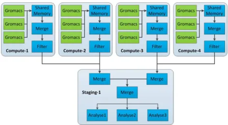
A typical scenario consists in extracting the data from each of the simulation processes, merge them locally on each node and perform some filtering and analy-sis computations in situ on a node-local helper core (Fig. 2). These computations are constrained to work on data from the local simulation processes unless they explicitly exchange data between nodes. For more global computations, the results are usually gathered on dedicated staging nodes (Fig. 3). Typically a ratio of 1/64 is applied between the staging nodes and the simulation nodes. Once the data are on the staging nodes, any kind of treatment can be performed without perturbing the simulation.
Our framework enables to map modules on helper cores or staging nodes simply by specifying a host name and a core in the Python script. The FlowVR daemon takes care of transparently moving the data to where they are expected.
Fig. 2 A node running simulation and in-situ processes. Each MPI process of the simulation (here Gromacs) is pinned to one core and the external analytics processes (filter and merge) and the FlowVR daemon share the dedicated helper core.
3.3 Coupling to the Gromacs Molecular Dynamics Simulation Engine Our scenarios currently rely on MD simulations executed with Gromacs. Gro-macs runs in parallel with MPI. It also supports other parallelisation paradigms (OpenMP, GPUs), not used in this paper. Gromacs20follows a master/slave organ-isation. The first MPI process (the master) loads the simulation, configures it and propagates all necessary information to the slaves. During the simulation, only the master can access the global state of the simulation. Each process is responsible only for the atoms contained inside its domain (called the home atoms). To write the trajectory and other backup files, a global state of the molecular system is gathered on the master node. This operation involves costly communications and synchronisations.
Fig. 3 Example of a simple yet classical live analysis deployment scenario using 4 compute nodes and 1 staging node. Data are first filtered at the node level (in situ), then they are sent to a staging node for further treatments (in transit). The output can be saved to disk or sent to a visualisation node to display the result.
We instrumented each MPI process of Gromacs with FlowVR. Every x it-eration each Gromacs process assembles a message containing the home atom positions and puts it on an output port. When data are extracted with FlowVR, the native Gromacs communications to gather data on the master before being written to files are suppressed. We also set an input port per process to retrieve external forces to be imposed to a selection of atoms. This port is activated only for the scenarios requiring steering.
3.4 Trajectory Analysis with MDAnalysis and Gromacs Tools
Software packages, such as VMD21, MDAnalysis22 or the built-in Gromacs tools20, enable the analysis of molecular systems and simulation trajectories. MDAnalysis is a Python library providing various classical algorithms to analyse structural and dynamic properties as well as membrane parameters. It provides a powerful selection language inspired by the CHARMM syntax. The Gromacs tools are small executables mainly designed to perform stream style post-treatments on a trajectory. It is possible for instance to filter a trajectory, recenter it on a particular residue or reconstruct a split system divided by the boundary conditions. We turned the MDAnalysis and the Gromacs tools into FlowVR modules, to be able to use these tools in an ExaViz application. Both libraries read trajectories from files and write results in output files. We extended their respective file formats with a new format able to read and write data from/to a FlowVR input/output port. To do so, we mapped the FlowVR module API to the traditional file I/O scheme. For live analysis we map these modules on staging nodes where all data are gathered as these tools expect to work on trajectories of the full molecular system.
3.5 Visual and PostMortem Analysis
Live processing is well suited for analysis that can be performed on a stream of time steps. For more general computations, it makes more sense to save the results to disk and post-process the data in a classical way. Postmortem processing is, of course, particularly useful to execute analysis that the scientist did not anticipate.
The ExaViz framework can actually be used for such computations. A trajec-tory reader module has been developed to read trajectories from file and output the needed time steps as FlowVR messages, these messages being processed by downstream analysis modules from the MDAnalysis or Gromacs tools for instance. The trajectory reader is responsible for navigating efficiently through the trajectory as well as filtering the information it delivers for the analysis modules. Its behaviour is controlled from outside by other modules that can send orders. For now, the reader is able to read compressed XDR files. Its efficiency relies on an index for all trajectory frames. This index is built once, the first time the trajectory is loaded into the reader. Several trajectories can be analysed simultaneously, enabling direct comparisons. The results from analysis modules are plotted and displayed in real-time.
3.6 Access to Multiple Interchangeable Visualisation Environments Visualisation and navigation are two essential components that cannot be dis-sociated from any analytical process.We developed our own 3D visualisation component based on the HyperBalls algorithm23, but other 3D viewers could be supported, taking advantage of ExaViz modularity. Rapid prototyping of original visualisation algorithms can be performed within our UnityMol framework24.
We primarily target desktop environments. But we also developed a 3D viewer for immersive environments, from stereoscopic devices to Cave-like systems. Navigating into complex molecular systems is cumbersome. We propose cam-era positioning and path planning algorithms taking into account the geometric features of molecular complexes (see section 4.1).
4
Immersive and Interactive Simulations
In order to perform the scenarios presented in the previous section, especially during IMD experiments, providing assisted navigation into a complex 3D molec-ular system is a crucial point before steering a target. In this part we present our contribution about navigation paradigms for molecular content exploration, that we experimented with in a desktop as well as in a Cave-like virtual environment25. Next we especially point out the advanced techniques we applied to provide an immersive collaborative context for simulation analysis, and the methodological and technical aspects underlying the steering of a simulation in progress.
4.1 Content-aware/Task-aware Navigation
Many large biological 3D structures are constructed around specific symmetry layouts26. Symmetry is not only a spatial feature of molecular complexes but it also plays a significant role for the stability and the function of such complexes. Symmetries found among large molecular complexes can be used as guidelines
to extract pertinent navigation paths. A few examples of symmetric complexes found in the cell are illustrated in Figure 4.
Fig. 4 Several types of symmetries found in molecular complexes. (A) GLIC, transmem-brane protein composed of 5 components with a single central symmetry axis. On the left, top view of the protein, on the right, side view. (B) Virus capsid with two types of components presenting a symmetry center overlaying the gravity center of the virus. (C) Tubulins assembling to shape a microtubule with a screw-like symmetry.
From these geometric features, we can anticipate certain specific navigation paths that would drive the user during the exploration of a molecular structure. The symmetry information we use all along our navigation paradigms are provided as a mandatory step right before any initiation of the visualisation process. It consists of a center or symmetry axis and a list of angles/translations linking each symmetry-related monomer of the molecular system studied. Symmetry information can be manually extracted or calculated by off-line analysis tools such as SymD27.
4.1.1 Camera Path for Molecular Exploration. To maintain a uniform and coherent point of view for the user, the symmetric nature of the complex is used. More particularly, a symmetry axis (or center for specific cases) is extracted from the 3D structure of each complex, in a manual or automated way. The symmetry axis is considered as the link between the ”floor” and the ”roof” of the virtual scene and the protein of interest is observed and explored following the metaphor of a tower28.
Circular paths around the structure are set up based on the symmetry axis and the bounding box of the protein. The up vector of the camera stays parallel to the symmetry axis all along the navigation and always faces the symmetry axis/center. Camera orientations and movements are then directly set with respect
Fig. 5 View of navigation paths when a symmetry axis (in red) has been detected. The molecular complex is coloured by chain and several examples of possible paths are rendered in light grey. When constrained, the camera follows these paths for which the radius is changing according to the camera distance to the symmetry axis. At any moment, the camera is facing either the center of the symmetry axis or one of its end points when the camera reaches the upper or lower parts of the navigation area (semi-circular paths).
to the relative position of the camera and the symmetry axis/center. Additional exploration paths along the symmetry axis may exist when a pore or a tunnel are present in the molecular complex. The GLIC pore example is illustrated in Figure 5.
4.1.2 Semi-Automatic Point of View Extraction. We developed an algo-rithm to compute the least occluded position to place the point of view and observe a given region of interest. Starting with the center of an area identified by the user, a sphere is created around this point with a radius matching a configurable distance between the camera and the target. From each element of the sphere surface, a ray is cast toward the target. If a ray crosses a cell of the grid with an atom in it, the grid element corresponding to a surface starting point is considered as occluded. At the end, each element of the surface is associated to a 2D table and we extract the area with less occluded neighbours (Figure-6(a)). The centers of these areas, once re-transformed into 3D coordinates, yield the observation points with the least occlusions to observe the target (Figure-6(b)). The user is then able to choose among the optimal points of view by modifying the position and the orientation of the camera.
4.1.3 Navigation Jumps between Symmetry Related Equivalent Positions. A frequent exploration task is to visualise a specific region of a molecular system, repeated along symmetry-related positions, for example the five monomers of the GLIC receptor. The movements to reach these regions involve quick and precise motions to be performed in order to simultaneously keep some spatial landmarks and reach the appropriate point of view in the middle of thousands of particles. The possibility to jump from one monomer site to another in a smooth and quite instantaneous way is particularly interesting for the comparison of binding sites or dynamic structures involved in complex stability. Targeting a specific region of a monomer includes four steps implemented in our navigation paradigm: face
Fig. 6 View of the rendering process used to extract the best point of view when targeting a precise atom (in red) in a molecular system. (a) In white, all the points that belong to a sphere of a radius matching the distance between the target and the future camera position. The center of the largest cluster (white sphere) is output as the best point of view to visualise the target. (b) Camera view when its position is brought to the white sphere location shown in (a).
the region of interest using guided navigation features (Figure 4), selection of the interesting area before computing the best point of view (as presented in the previous section), save the point of view, and jump to the next monomer thanks to the available symmetry information.
4.2 Immersive and Collaborative Exploration
Most of the navigation features evoked in the previous section were motivated by the immersive context offered by virtual environments. These are especially adapted for interactive simulations and for postmortem simulation analysis for sev-eral reasons. The stereoscopic 3D rendering allows to explore complex biological structures that are intrinsically 3D objects. Moreover head-tracked stereoscopy allows the user to turn around the 3D object and explore it from different points of view just by natural walking in the immersive system, as in real context. When navigation is not required, head-tracked stereoscopy features allow the user to fo-cus his molecular structure without being disturbed by interaction devices required to navigate within a virtual scene. We highlight the fact that these navigation features were designed to be independent from the nature of the control device. In this way, mouse and keyboard used as input devices to control navigation in a desktop context are substituted by virtual reality devices such as 3D mouse, Joystick and advanced head-tracking techniques to control navigation features in an immersive context.
It is important for a scientist to easily share an experimental result or obser-vation. Immersive environments address this question by implementing multi-collaborative techniques that allow to share a working space between two users with their own point of view. To do so the active and passive filtering capability of a Cave-like system has been used and developed in order to provide the col-laborative capacity while gathering the best navigation conditions to a group of users. Like the advanced systems proposed by Froehlich29, our immersive system is able to provide two head-tracked stereoscopic points of view, with each user having his/her own molecular representation of the same structure. This setup
provides the first basic features for collaborative work where the real hands of the users are co-localised with the 3D pointed virtual object, and then the pointing place is coherent for the two users’ points of view.
We can also extend our immersive environment with specific haptic devices for 3D interactive picking of atoms. A test case is shown in section 5.1.1 focusing on an interactive simulation. This provides proprioceptive feedback of the force that steers the simulation which in turn can drive user interaction with the simulation. We integrated an advanced haptic device that allows the user to access the whole workspace of the immersive environment, automatically following the user during the haptic picking of an atom (see Figure 7(b)).
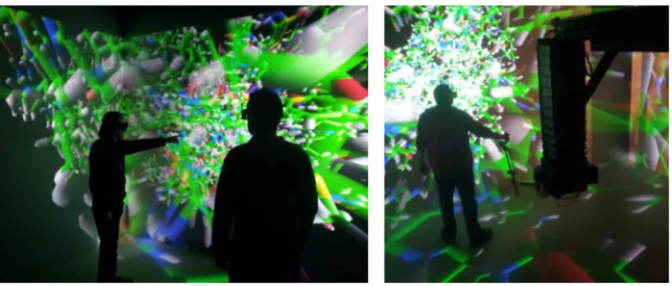
Fig. 7 (a) Two users in our collaborative Cave-like system, each with their own head-tracked 3D point of view, allowing pointing to discuss about a shared 3D object. (b) Our advanced haptic device allows users to access the whole workspace of the immersive system.
4.3 Human Steering
A convenient task to perform interactively is to steer a system, possibly in an immersive context (see Figure 7(b)). This allows the user to immediately adapt and react to the behaviour of the molecular system and draw benefit from human intuition and instantaneous decision-making. Hence even very complex manip-ulations can be carried out. However, the concept of IMD5,30 is limited by the simulation speed and human time. Typically, with a simulation running at 500 Hz and an integration step of 2 fs, we can only simulate about 1ns in a 15 min interactive session. This considerably limits the range of possible applications since most biologically relevant phenomena require at least several hundreds of nanoseconds or even much longer timescales to occur. To mitigate this problem, significant forces are sometimes applied to speed up the biological process with the risk to affect the correctness of the simulation. This important issue will be discussed in more detail in subsequent paragraphs about in situ steering.
From a technical point of view, traditionally, an IMD system sends forces to one process of the simulation (called the master node) and retrieves the atom positions for visualisation. This scheme implies that the simulation broadcasts the user forces to all the other processes and gathers the atom positions at each step,
which are two costly operations. Experiments have shown that this scheme does not scale up to large systems and/or high levels of parallelism. In previous work6, we used the coupling method described in section 3.3. The key feature of this method is that the broadcast of the forces and the gathering of the atom positions are done asynchronously outside of the simulation. This ensures a minimal impact on the simulation performance by avoiding costly blocking operations during the simulation execution and a severe bottleneck on the master node. With this system, we were able to steer molecular systems up to 1.7 million atoms at about 25 Hz using 384 cores for the simulation with a cost of 17% on the simulation performance (compared to Gromacs at equal core count without IO).
In contrast to human IMD steering, the SMD approach4uses a similar concept but the forces are described by a script or algorithm. This allows to run long simulations in batch mode on a cluster. However, scripting complex paths can be very tedious compared to a direct interactive steering.
5
In Situ Steering, Reporting and Analysis
We present two live analysis scenarios. The first one draws a continuum between IMD and SMD approaches. We propose to automatically steer a molecular system based on a user defined path captured through a preparatory IMD session. The second one is a more classical scenario. We show that it is possible to filter and save to disk a trajectory ready to use for postmortem analysis, with a significant performance gain compared to Gromacs’s native IO system. This step addresses the frequent tasks of either reducing the trajectory size or increasing the saving frequency for specific trajectories of subsystems of interest.
5.1 Live SMD Steering
5.1.1 Moving from IMD to SMD. Our method relies on three steps. First, the user performs an interactive session with our IMD system, most likely applying a level of force that is too high to be realistic. However, this session allows the user to already eliminate some possible paths. Our previous work6demonstrated that our IMD system is able to run large molecular simulations interactively allowing a wide variety of scenarios. Next, based on the trajectory extracted from this interactive session, the user defines a series of key points on the path called targets. Once these targets are identified, the user can relaunch his simulation in SMD mode. In this mode, the steered complex is pushed successively toward the targets.
To automatically push the steered complex, we add to our IMD system a component called TargetSystem. This component has three main functionalities: tracking the steered complex, tracking the position of the targets and emitting new forces. At each output step, the TargetSystem receives the atom positions from the simulation by the same communication channel as the visualization in the IMD system. The current position of the steered complex and the targets are extracted from the atom positions using the selection capabilities of MDAnalysis. The direction of the emitted force is then defined by the difference of positions between the current active target and the center of mass of the steered complex.
During the automated sessions, several measures are displayed to provide a quick overview on the state of the steering process. Information such as the current
level of applied forces, distance to the next target or the estimated time remaining until completion allow the user to see easily the behavior of the steering process and to decide quickly if the system can continue on its own. The guiding system also forces Gromacs to produce a checkpoint file when the steered particles reach a target making it easily possible to resume an automated session at a certain point. In a batch mode session, this information is gathered inside a simple report file accessible by the scientist at any time of the simulation.
Note that this application can run both in batch mode or during an interactive session. In an interactive session, the system behaves like a traditional IMD system with visualisation and the use of a haptic device in addition to the TargetSystem component. The user has the possibility to activate the automatic steering or not, depending on his needs. In the case where the automatic steering is activated, the user still has the possibility to apply forces by himself, as the forces emitted by the haptic device are prioritised over the automated forces. This feature is very useful in case the steered complex gets stuck on its path. Manual guidance allows the user to complement the automated system and reposition the complex in the proper path, or find an alternative possible path. To run in batch mode, we simply disconnect the visualisation and haptic device from the application. The rest of the application can run without any intervention from the user.
5.1.2 Experiments on the FepA Channel. We run our system on the Grid-5000 testbed as computational cluster plus a visualisation node. The hardware used for the visualisation is a Xeon E5530 quad core CPU at 2.40 GHz with a GeForce 680 GTX graphics card. The computational cluster used is composed of 72 nodes, each node running 2 Xeon E5520 quad core CPU at 2.27 GHz, 24 Gbits RAM. Communications between the computational cluster nodes go through a QDR Infiniband fabric (40 Gbits/s) while we only have a DDR (20 Gbits/s) Infiniband interconnection between the computational cluster and the visualisation node.
As a use case we extend our previous experiments on the FepA channel. In6,
we found two possible paths with our IMD system, but those required a level of force considered too high to be realistic (2000 pN per atom). We tried interactively to follow a similar path with a lower amount of force, however this was difficult without a visual guide indicating the previously found path and because of the slow motion of the complex.
To run the simulation we used 16 nodes from the computational cluster with 7 cores per node for the simulation and 1 dedicated core. The dedicated core runs the FlowVR Daemon, a merger to aggregate the data from the 7 local Gromacs processes, an atom filter to avoid sending unwanted atoms to the visualisation such as the water molecules, and an iteration filter to send only one frame every
xframes. The combination of both filters at the node level ensures a minimum network traffic minimising our impact on the simulation performance. The other components (visualisation, haptics, targeting system) run on the visualisation node which is our staging node. With this setup we obtain a simulation running at 230 Hz with data sent every 10 frames to the staging node.
In our first experiments, we launched our system with the predetermined path and the same amount of force as in our IMD session (2000pN per atom). We have been able to reproduce this experiment multiple times automatically. Surprisingly the automatic system is faster than the human guided one to perform the same
experiment (3 minutes for the user against 2 min for the automated system). This is most likely due to the fact that the human constantly deviates from the path whereas the automatic system stays on target. As a second step, we launch the same setup with 1500 pN per atom, a level of force for which we could not complete the process in a reasonable time interactively. Our system was able to follow the same path as the interactive one. However the complete experiment took about 10 minutes to complete. During the experiment we saw that the complex was stuck at certain steps. After a period of time, the side chains reoriented in a way that allowed the complex to continue its path. As in the previous experiments, we were able to perform the same run multiple times without human intervention. We tried the same experiment with 1000pN per atom using the same setup as before. In this case, we encounter some problems related to the deformation of the channel over time. After 15 min, the channel starts to translate and slightly modify its shape. As our path definition is for now absolute in space, the path becomes irrelevant after these transformations. However we were able to push the complex inside the channel in the first period of the simulation where the channel is stable compared to its initial state. These observations tend to indicate that the complex could go through the entire path provided enough time.
5.1.3 Discussion. With long simulations arise two major problems in our guiding system: conformational changes and jumps of the molecule due to the periodic boundary conditions. These issues pose mainly technical challenges. A more fundamental issue relates to the correctness and repeatability of such experiments.
To solve the conformational problem, we are currently working on a way to describe the target positions relative to some reference atom positions in the system. In this way, the target position would follow the same transformation as the reference atoms. However, there is no obvious way to describe a relative position which would be robust enough in all cases. For instance, if we take as reference several residues of the backbone of the channel, our target will follow the global movement of the channel but will miss the local changes inside the channel. On the other hand, if we take local points only to describe the target, the target position might become unstable if one of the reference points moves significantly.
A mandatory condition to set up targets properly is to preserve the integrity of a reference structure. However the periodic boundary conditions of the sim-ulation can split this structure into one or several image boxes anytime during the execution. This raises two major problems for the targeting system : first the computation of the target position must take into account the various image domains of the simulation, second the emitted force direction must also take into account this periodicity. To solve this problem outside of Gromacs, extra information are required : the bounding box shape of the simulation to detect and undo the jump into image space, and topological information of the system to preserve the integrity of a reference structure. The trj conv tool from Gromacs is commonly used to post-process a trajectory based on these information. It possesses various useful functionalities to rearrange a trajectory like centering, correcting the jumps and splits due to periodic boundary conditions, filtering atoms, etc... A promising solution to our problem is to integrate this tool in our framework and to plug it with the correct options between the simulation and the
targeting system. This way, the targeting system can simply ignore the periodic boundary conditions since they are corrected by the trj conv module. Note that this is possible because trj conv only translates atoms but does not apply any rotation. Therefore the direction of the emitted forces can be directly sent to the simulation. Otherwise it would be necessary to undo the rotation of the emitted force before sending it to the simulation. This solution is currently tested on the FepA channel experiment. A fundamental question arises from the level of force applied to the simulation system. Although hundreds to a few thousands of pN have previously been used for similar experiments on ligand dissociation31,
peptide membrane penetration32, glucose transport33or substate entry into an active site34, the applied forces remain almost an order of magnitude higher than forces encountered in natural biological systems. Therefore the correctness of the results should be checked very carefully, for instance by carrying out numerical experiments with various levels of forces and by repeating an experiment several times. Repetition is particularly important for human guided experiments, and we typically carry out 3 to 10 replica to account for the inherent variability of the human intervention.
5.2 Post Treatment and Analysis with Gromacs and MDAnalysis Tools Handling of trajectory files is a major problem for long simulations. A trade-off must be found between the trajectory file size, the impact of I/O operations on the simulation performance and the timescale of the biological phenomena. With this application we propose a possible solution for these three points. The goal is to enable the scientist to output a complete trajectory at a common interval and at the same time much smaller filtered trajectories but with a higher output frequency.
5.2.1 Application Setup. In this experiment we use the GLIC ion channel as application example. One of the points of interest of this simulation is the presence or not of water inside the channel pore and the shape of the pore-lining M2 helices according to the presence of water. Based on this analysis, we would like to produce a lightened trajectory with only the M2 helices, the 1000 closest water molecules from the channel center and the ions in the system. The trajectory should be centered on a residue inside the channel to avoid shifting of the trajectory. Overall, each frame is reduced from 143k atoms to about 3k atoms. To filter this trajectory we use the Gromacs tools trj order and trj conv integrated within our framework. Simultaneously, a complete trajectory is produced at a normal output frequency since not all analyses could run with the light trajectory. We expect the
trj ordertool to run slower than the simulation output rate since heavy operations such as atom sorting are required to select the 1000 closest water molecules. To tackle this problem, we create multiple instances of the trj order module and add a rooting component. This rooting component dispatches incoming frames on the
trj ordermodules in a round robin fashion. A similar component is placed after the trj order modules to reorder frames and send them to the trj conv module.
The experiments ran on Froggy, a 138 compute nodes cluster from the Ciment infrastructure. Each compute node is equipped with 2 eight core processors Sandy Bridge-EP E5-2670 at 2.6 GHz, 64GB of memory. Nodes are interconnected through a FDR Infiniband network. FlowVR 2.1 and Gromacs 4.6 are compiled with Intel MPI 4.1.0. For all experiments Gromacs runs a simulation with the
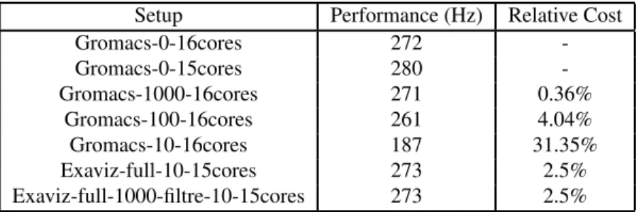
Setup Performance (Hz) Relative Cost Gromacs-0-16cores 272 -Gromacs-0-15cores 280 -Gromacs-1000-16cores 271 0.36% Gromacs-100-16cores 261 4.04% Gromacs-10-16cores 187 31.35% Exaviz-full-10-15cores 273 2.5% Exaviz-full-1000-filtre-10-15cores 273 2.5%
Table 1 Gromacs performance with native writing methods compared to our framework (higher is better). The GLIC model (143k atoms) is used with a fixed configuration of 16 nodes (256 cores max). gromacs-X -Y cores write every X step with the Gromacs native writing method using Y cores per node. exaviz-full-X -filtre-Y -Zcores writes a complete frame every X frames and a filtered frame every Y frames with our framework writing method using Z cores per node. Relative costs are given compare to the same cores counts.
GLIC model composed of about 143k atoms and with PME nodes activated. We use up to 32 nodes for the simulation as compute nodes and one extra node as staging node. On each compute node we set 15 Gromacs MPI processes and one dedicated core. The dedicated core runs the FlowVR daemon and a merger. The data are then aggregated toward the staging node. On the staging node, we run a
trj convinstance with no specific option to output a complete trajectory in XTC format. Another tjr conv instance and a trj order filter are set up to produce the filtered trajectory. Every 10 simulation steps, atom positions are extracted from the simulation and sent to the staging node. The pipeline generating the filtered trajectory receives each of the extracted frames and writes them. The trj conv module for the complete frame outputs a frame only every 100 received frames which corresponds to a usual output frequency of every 1000 frames in Gromacs.
5.2.2 Output frequency evaluation. Table. 1 shows the Gromacs running frequency for various configurations. 16cores (resp.
Gromacs-0-15cores) indicates the performance of Gromacs running on all the 16 cores
available per node (resp. 15 cores) and without performing any IO. These values set the upper performance bounds we should try to stay close to when activating data saving. When Gromacs writes the atom positions to disk every 10 steps the performance drops significantly (31% drop on Gromacs-10-16cores).
The line exaviz-full-10-15cores reproduces the Gromacs file writing pattern with FlowVR. Data are gathered on the staging node and written in an XTC file with the Gromacs trj order tool modified as described in section 3.4. The curve
exaviz-full-1000-filtre-10-15coresreproduces Gromacs file writing every 1000
steps and the writing of the filtered trajectory every 10 frames. Five trj order tools were created in parallel to absorb the production rate. Both exaviz tests have the same cost on the simulation, which is expected since the major cost is the data transfer that is the same in both cases. Overall, these results show that our writing method is very close to Gromacs-0-15cores (2.5% drop) despite the very high output frequency from the simulation (1 frame every 10 frames).
5.2.3 Scalability evaluation. In these experiments, we evaluate the scalabil-ity of our framework to write a trajectory at high frequency. Due to its relatively
Fig. 8 Gromacs performance with various writing methods. The benchmark model (2M1 atoms) is used. gromacs-X -Y cores write every X steps with the Gromacs native writing method using Y cores per node. exaviz-full-X -Y cores write a complete frame every X frames with our framework method using Y cores per node.
small size, the GLIC system is not suitable to scale well on a large number of cores. Instead we use a molecular system specifically designed to scale up to several thousands of cores. We run a Martini simulation35with a patch of 54000 lipids representing about 2100000 coarse grained particles. In the previous section, we demonstrated that our framework enabled to produce extra trajectories at no extra cost. In this experiment we produce one complete trajectory at high frequency.
Fig. 8 shows the Gromacs running frequency on our benchmark model. The curve notations follow the same conventions as previously. In this case, the curve
Gromacs-100-16coresscales poorly beyond 512 cores due to the very important
amount of global communication to write the trajectory. The curve
exaviz-full-100-15coresdemonstrates that our framework is able to scale up to 1664 cores
even with this size of molecular model and output frequency. We note a slight cost compare to Gromacs-0-16cores which is mainly due to the reserved dedicated core on each node and the extra network traffic to gather the data on the staging node.
5.2.4 Discussion. These experiments demonstrate two important features of our framework to help resolve the necessary tradeoff for trajectory writing. First, it is possible to write multiple trajectories with filtering at the same cost of writing one complete trajectory. This alleviates the trajectory size problem. Second, we are able to output trajectories at a high rate, even for the complete trajectory, at the cost of one dedicated core per node, considerably improving the Gromacs writing performance even on a high number of cores.
6
Visual and PostMortem Analysis
In addition to the 3D visualisation of the molecular system, the scientist can add several other windows to complement his visual analytics dashboard. The results of the analysis performed on staging nodes can be streamed to the visuali-sation node for on-line plotting. These features are available for live as well as postmortem analysis. For postmortem analysis, extra features enable to navigate
through or select frames on one or several trajectories. 6.1 Trajectory Player
The trajectory player module is a graphical interface that allows the user to navigate through the trajectory. The user interface resembles a DVD player where it is possible to go forward and backward, to accelerate, slow down or pause the reading. It is possible to loop on a selected part of the trajectory. This module mainly controls the behaviour of the trajectory reader described in Section 3.5. The trajectory reader is connected to analysis and visualisation modules and provides the same functionalities as in an in situ and interactive context for atom filtering. The quality of the postmortem analysis relies on the ability of the trajectory reader to quickly access the different trajectory frames. For now, we made experiments on trajectories ranging from hundreds of Megabytes to several Gigabytes and we obtained a random access to the frames ranging from 0.01s for small systems (about 10000 atoms) to 0.2s for several million atom systems. However, the current trajectory reader must be improved to handle very large trajectories of several Gigabytes. This can be achieved by using techniques such as those described by Stone et al36within our framework.
6.2 Real Time Plots
It is common to use families of function graphs in the visual analysis process37. Usually, when the scientist requests a trajectory analysis, he only gets the result at the end of the trajectory processing. If this may be acceptable for postmortem analyses, it does not enable to monitor the simulation during its execution. ExaViz enables to plot the streams of data received from analysis modules in real time. The scientist gets the results as soon as available, enabling him to make putative decisions for further analyses or re-parametrisation of the trajectory.
To implement this feature in the FlowVR layer, we connect a module for each analysis script and a module for displaying graphs called GraberStats.
GraberStatsis based on the Qwt library. Besides a framework for 2D plots, Qwt provides scales, sliders, dials, compasses, thermometers, wheels and knobs to control or display values, arrays, or ranges of type double. It is possible to display multiple plots on the same graph to superimpose the results and to compare them quickly. Note that this module is available in any context except batch mode. A future version will allow to write the graphs into images to be compatible with batch mode constraints.
An example was performed for the analysis of the GLIC ion channel. This structure has both open and closed states, the transition mechanism between different states is unknown. Understanding this transition is crucial as potentiating molecules such as anesthetics and alcohols are believed to affect transition barriers or the relative free energy of states. To investigate these dynamics, we have performed extensive simulations of GLIC. Pore hydration seems to be related to the pore organisation and mainly the pore lining helix M2. To characterise the conformation of this helix, we have implemented two MDAnalysis scripts.
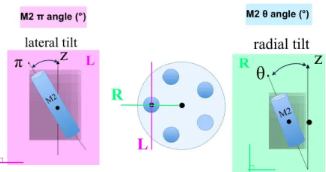
First, we have computed the tilt angles, and decomposed them in two angles: the radial (θ) and lateral (π) tilt angles of M2 around its center of mass with respect to the overall channel pore axis (Fig. 9(a)). These angles are useful to
(a) the radial (θ) and lateral (π) tilt angles of M2 around its center of mass with respect to the overall channel pore axis
(b) the number of water molecules in the pore zone between the two hydrophobic residues I9’ and I16’
Fig. 9 Analysis examples for the GLIC ion channel case which is an ion channel with a central pore formed by its five identical subunits as shown in Figure 4(a).
describe the state of the pore. Then, we counted the number of water molecules in the pore zone between the two hydrophobic residues I9’ and I16’ (Fig. 9(b)). This region was the most affected by the pore dewetting. These two scripts have been applied on a trajectory during the reading by the trajectory player. The results were displayed on three graphs shown in Fig. 10. In the former there is a curve for each M2 helix indicating the lateral angle around its center of mass. In the second it is the same for the radial angle. Finally on the last are the numbers of water molecules within the pore. To speed up the analysis process, we use the same strategy as in Section 5.2.1 and deploy multiple instances of the analysis modules if enough CPU resources are available. Note that these analyses are performed in a post-mortem context for this example however they can be computed in situ as well.
6.3 ”Smart” Selections Linking Analysis Data to Trajectory Frames To make the analysis process less cumbersome, it is common to investigate sub-groups of the full simulation dataset38. We integrated the possibility to select a pool of frames in a graph, and to trigger the computation of a new plot for this selection. Such selections can be repeated to refine the analysis. Selections
Fig. 10 ExaViz visual interface with the TrajReader and GraberStats modules, and two analysis scripts for the GLIC ion channel. The user selects several frames based on the frame numbers (x axis) and the analysis values (y axis).
can be done by choosing a range in the frame numbers (x axis) and/or in the analysis values (y axis) directly in a graph window (Fig. 10). Once the selection is made, zoom operates in all the graphs so that results are available only for the selection. The resulting frame numbers are sent back to the TrajReader to reduce the trajectory to the selected frames. This sub trajectory can be replayed without recomputing the analysis since the results do not change from the initial trajectory. To run new analysis on this sub trajectory, the scientist has to save the selected frame number and relaunch the application with a new analysis pipeline and the selected frames loaded.
In the GLIC example where we plotted the number of water molecules in the pore, the scientist could for instance select all the frames that do not have any water molecules in the pore. The resulting trajectory will therefore enable the visualisation of the protein in a closed and dewetted state, allowing to focus on any interesting features.
6.4 Concurrent Analyses on Multiple Trajectories
As shown on Fig. 10, the GraberStats module is able to display multiple curves in the same window. This allows an easy comparison between results. Based on this feature, we are able to provide a multi trajectory support. To do so, we simply duplicate the analysis pipeline segment from the TrajReader to the analysis modules and connect each output port of the analysis modules to the GraberStats instances. Then the scientist simply has to attach both data sources to the same window to obtain a comparative view of multiple trajectories.
Fig. 11 shows the application graph that computes the number of water molecules inside the Glic channel from N different trajectories. The full analysis
Fig. 11 Example of a multi trajectory application. The number of atoms in the Glic channel is counted for N simulations and sent to the GraberStats module. The analysis pipeline is simply duplicated to handle multiple trajectories.
pipeline is duplicated as many times as trajectories are available for analysis. To support the selection of frames from the GraberStats window, the developer has to reconnect each selection output associated to a data source to its rightful origin, i.e. to the correct TrajReader. Note that this application scheme would be exactly the same for the in situ analysis of multiple simulations, except for the TrajReader to be replaced by multiple simulations.
7
Conclusion
The ExaViz framework is dedicated to the extraction, analysis and visualisation of MD simulation trajectories. Modularity is the key concept ExaViz is built upon. The adopted dataflow, component oriented approach enables to reuse modules in different contexts, to distribute components at large scale to enable parallel executions, to encapsulate existing libraries or to couple to existing MD simulation codes. We developed MD specific modules for different levels of the analytics pipeline, from the trajectory reader or in situ data extraction, to analysis, real-time plotting, visual navigation in 3D molecular systems. From the same application base, we show that the scientist can set up different scenarios for interactive, live or postmortem trajectory analysis and steering.
To be productive, the analytics process requires a tight interaction between the expert and the application. The environment needs to be able to dynamically adapt itself to the user needs. ExaViz provides some dynamic behaviours, but it remains an active investigation topic to identify which ones are needed, and how to support them. We are also exploring how a semantics modeling of the manipulated data could enhance the analytics process, for instance by extending the concept of smart selection. We plan to publicly release the ExaViz code in the near future and hope it will foster the development of new scenarios and features.
8
Acknowledgements
This work was supported by the French Agency for Research (Grant ”ExaViz”, ANR-11-MONU-003) and the ”Initiative d’Excellence” program from the French State (Grant ”DYNAMO”, ANR-11-LABX-0011). Experiments were performed on the Grid’5000 experimental testbed (https://www.grid5000.fr), and the Froggy platform of the CIMENT infrastructure (https://ciment.ujf-grenoble.fr//). We
thank Dr. Samuel Murail and Benoist Laurent for stimulating discussions about the analysis of the GLIC system.
References
1 J. C. Phillips, R. Braun, W. Wang, J. Gumbart, E. Tajkhorshid, E. Villa, C. Chipot, R. D. Skeel, L. Kal and K. Schulten, Journal of Computational
Chemistry, 2005, 26, 1781–1802.
2 B. Hess, C. Kutzner, D. van der Spoel and E. Lindahl, Journal of Chemical
Theory and Computation, 2008, 4, 435–447.
3 G. Zhao, J. R. Perilla, E. L. Yufenyuy, X. Meng, B. Chen, J. Ning, J. Ahn, A. M. Gronenborn, K. Schulten and C. Aiken, Mature HIV-1 Capsid Structure
by Cryo-electron Microscopy and All-Atom Molecular Dynamics, 2013.
4 S. Izrailev, S. Stepaniants, B. Isralewitz, D. Kosztin, H. Lu, F. Molnar, W. Wrig-gers and K. Schulten, Computational Molecular Dynamics: Challenges, Meth-ods, Ideas, 1998, pp. 39–65.
5 J. E. Stone, J. Gullingsrud and K. Schulten, Proceedings of the 2001 sympo-sium on Interactive 3D graphics, New York, NY, USA, 2001, pp. 191–194. 6 M. Dreher, M. Piuzzi, A. Turki, M. Chavent, M. Baaden, N. F´erey, S. Limet,
B. Raffin and S. Robert, International Conference on Computational Science, ICCS 2013, 2013.
7 J. Thomas, Illuminating the Path: The Research and Development Agenda for
Visual Analytics, IEEE Computer Society Press, 2005. 8 J. J. LaViola, Jr., SIGCHI Bull., 2000, 32, 47–56.
9 E. Lindahl, B. Hess and D. van der Spoel, J Mol Model, 2001, 7, 306–17. 10 H. J. C. Berendsen, J. P. M. Postma, W. F. van Gunsteren and J. Hermans,
Intermolecular Forces, 1981, pp. 331–342.
11 H. J. C. Berendsen, J. P. M. Postma, W. F. van Gunsteren, A. DiNola and J. R. Haak, The Journal of Chemical Physics, 1984, 81, 3684–3690.
12 J. D. Faraldo-Gomez, G. R. Smith and M. S. P. Sansom, Biophys J, 2003, 85, 1406–20.
13 J. D. Faraldo-Gomez, L. R. Forrest, M. Baaden, P. J. Bond, C. Domene, G. Patargias, J. Cuthbertson and M. S. Sansom, Proteins, 2004, 57, 783–791. 14 A. E. Garcia and K. Y. Sanbonmatsu, Proc. Natl. Acad. Sci. U.S.A., 2002, 99,
2782–2787.
15 J. Allard, J.-D. Lesage and B. Raffin, Presence: Teleoperators and Virtual
Environments, 2010, 19, 142–162.
16 H. Yu, C. Wang, R. Grout, J. Chen and K.-L. Ma, Computer Graphics and
Applications, IEEE, 2010, 30, 45–57.
17 F. Zheng, H. Zou, G. Eisnhauer, K. Schwan, M. Wolf, J. Dayal, T. A. Nguyen, J. Cao, H. Abbasi, S. Klasky, N. Podhorszki and H. Yu, IPDPS’13, 2013. 18 M. Dorier, G. Antoniu, F. Cappello, M. Snir and L. Orf, CLUSTER - IEEE
International Conference on Cluster Computing, 2012.
19 W. Gu, G. Eisenhauer, K. Schwan and J. Vetter, In Ninth International Confer-ence on Parallel and Distributed Computing and Systems (PDCS’97), 1998, pp. 699–736.
20 S. Pronk, S. Pall, R. Schulz, P. Larsson, P. Bjelkmar, R. Apostolov, M. R. Shirts, J. C. Smith, P. M. Kasson, D. van der Spoel, B. Hess and E. Lindahl,
Bioinformatics, 2013, 29, 845–854.
21 W. Humphrey, A. Dalke and K. Schulten, Journal of Molecular Graphics, 1996, 14, 33–38.
22 N. Michaud-Agrawal, E. J. Denning, T. B. Woolf and O. Beckstein, J. Comput.
Chem., 2011, 32, 2319–2327.
23 M. Chavent, A. Vanel, A. Tek, B. Levy, S. Robert, B. Raffin and M. Baaden,
Journal of Computational Chemistry, 2011, 32, 2924–2935.
24 Z. Lv, A. Tek, F. Da Silva, C. Empereur-mot, M. Chavent and M. Baaden,
PLoS One, 2013, 8, e57990.
25 C. Cruz-Neira, D. J. Sandin, T. A. DeFanti, R. V. Kenyon and J. C. Hart,
Commun. ACM, 1992, 35, 64–72.
26 D. S. Goodsell and A. J. Olson, Annual review of biophysics and biomolecular
structure, 2000, 29, 105–153.
27 C. Kim, J. Basner and B. Lee, BMC Bioinformatics, 2010, 11, 1–16.
28 A. Hanson, E. Wernert and S. Hughes, Scientific Visualization: Dagstuhl ’97 Proceedings, IEEE Computer, 1997, pp. 95–104.
29 A. Kulik, A. Kunert, S. Beck, R. Reichel, R. Blach, A. Zink and B. Froehlich,
ACM Trans. Graph., 2011, 30, 188.
30 J. E. Stone, A. Kohlmeyer, K. L. Vandivort and K. Schulten, Proceedings ISVC’10, Berlin, Heidelberg, 2010, pp. 382–393.
31 D. Long, Y. Mu and D. Yang, PLoS ONE, 2009, 4, e6081.
32 S. Yesylevskyy, S. J. Marrink and A. E. Mark, Biophys. J., 2009, 97, 40–49. 33 A. Sheena, S. S. Mohan, N. P. Haridas and G. Anilkumar, PLoS ONE, 2011, 6,
e25747.
34 S. K. Ludemann, V. Lounnas and R. C. Wade, J. Mol. Biol., 2000, 303, 813– 830.
35 S. J. Marrink, H. J. Risselada, S. Yefimov, D. P. Tieleman and A. H. de Vries,
The Journal of Physical Chemistry B, 2007, 111, 7812–7824.
36 J. E. Stone, K. L. Vandivort and K. Schulten, ISVC (2), 2011, pp. 1–12. 37 Z. Konyha, K. Matkovic, D. Gracanin, M. Jelovic and H. Hauser, IEEE
Transactions on Visualization and Computer Graphics, 2006, 12, 1373–1385.
38 C. Turkay, A. Lundervold, A. Lundervold and H. Hauser, Visualization and