HAL Id: hal-01420311
https://hal.inria.fr/hal-01420311
Submitted on 20 Dec 2016
HAL is a multi-disciplinary open access
archive for the deposit and dissemination of
sci-entific research documents, whether they are
pub-lished or not. The documents may come from
L’archive ouverte pluridisciplinaire HAL, est
destinée au dépôt et à la diffusion de documents
scientifiques de niveau recherche, publiés ou non,
émanant des établissements d’enseignement et de
Metro Energy Optimization through Rescheduling:
Mathematical Models and Heuristic Algorithm
Compared to MILP and CMA-ES
David Fournier, Thierry Martinez, François Fages, Denis Mulard
To cite this version:
David Fournier, Thierry Martinez, François Fages, Denis Mulard. Metro Energy Optimization through
Rescheduling: Mathematical Models and Heuristic Algorithm Compared to MILP and CMA-ES .
[Research Report] Inria Saclay Ile de France. 2016. �hal-01420311�
Metro Energy Optimization through Rescheduling:
Mathematical Models and Heuristic Algorithm
Compared to MILP and CMA-ES
IDavid Fourniera,b, Thierry Martineza, Fran¸cois Fagesa, Denis Mulardb
aInria Saclay - EPI Lifeware - 1 rue Honor d’Estienne dOrves - Campus de l’cole
Polytechnique 91120 Palaiseau (France)
bGeneral Electric Transportation ITS Delta - Tour Europlaza 28D5, 20 avenue Andr´e
Prothin 92063 Paris La D´efense Cedex (France)
Abstract
The use of regenerative braking is a key factor to reduce the energy consump-tion of a metro line. In the case where no device can store the energy produced during braking, only the metros that are accelerating at the same time can ben-efit from it. Maximizing the power transfers between accelerating and braking metros thus provides a simple strategy to benefit from regenerative energy with-out any other hardware device. In this paper, we use a mathematical timetable model to classify various metro energy optimization problems studied in the literature and prove their NP-hardness by polynomial reductions of SAT. We then focus on the problem of minimizing the global energy consumption of a metro timetable by modifying the dwell times in stations. We present a greedy heuristic algorithm which aims at locally synchronizing braking trains along the timetable with accelerating trains in their time neighbourhood, using a non-linear approximation of energy transfers. On a benchmark of the litterature composed of six small size timetables, we show that our greedy heuristics per-forms better than CPLEX using a MILP formulation of the problem with a linear approximation of the objective function. We also show that it runs ten times faster than a state-of-the-art evolutionary algorithm, called the covariance matrix adaptation evolution strategy (CMA-ES), using the same non-linear ob-jective function on these small size instances. On real data leading to 10000 decision variables on which both MILP and CMA-ES do not provide solutions, our dedicated algorithm computes solutions with a reduction of energy con-sumption ranging from 5% to 9%.
Keywords: Energy Optimization, Timetable Optimization, Regenerative
IThis article is an extended version of an article presented at the Railways 2014 conference
[1]
Email addresses: [email protected] (David Fournier),
[email protected] (Thierry Martinez), [email protected] (Fran¸cois Fages), [email protected] (Denis Mulard)
Braking, Mass Rapid Transit, Greedy Heuristics
1. Introduction
Energy consumption is a major issue for the future and has been the subject of increasing research activities over the last years. The total energy consumed in transportation is estimated to represent 27% of the world energy production [2]. In 2006, the London Underground consumed 1173 GW.h [3], representing 2.8% of the Great London total electricity consumption [4]. The transportation field is thus of particular importance and industrial companies try to optimize energy by different means, in particular in mass rapid transit such as metros.
Nowadays, almost all metros have energy regenerative braking systems. These devices turn the electric motors into generators during braking, and pro-duce electric energy. It has been shown that the raw energy discount provided by this technology is about 16.5% [5]. Some metros can directly use their own regenerative energy. Super capacitors allow much faster loads and unloads com-pared to classical batteries, and a metro equipped with super capacitors is able to collect the energy during braking, and give it back to the engine for its own accelerations [6]. The metros that cannot store their own regenerative energy can return it to the DC electrical network, but with important losses on long distances. The electrical substations (ESS) are the devices that convert AC to DC to feed the metro line. Some ESS are revertible and can convert the regen-erative power of trains to AC power. In this case, the energy regenerated by metros can be used in other parts of the metro line without important loss, or be sold back to the electricity provider. However, super capacitors, as well as revertible ESSs, are expensive equipment to buy and maintain, and may not be economically justified.
Another way to use the regenerative energy returned to the DC line, without requiring any extra equipment, is to synchronize the braking of a metro with the acceleration of another metro in its close neighbourhood on the DC line. This synchronization can be done, for instance, by modifying the departure and arrival times of the metros in the stations, in order to shift the acceleration phases to the deceleration phases of some other metros in their neighbourhood. The objective function may then combine two criteria: the minimization of power peaks, and the minimization of the global energy consumption during the day. A power peak occurs when too many metros are accelerating at the same time, which may cause two problems. First, a metro network is sized with some maximum power capacity. When the demand exceeds that threshold, a control system prevents the destruction of the electric equipment by a momentary shut down of a part of the network, dropping the quality of service. Second, more than 80% of metro companies pay their energy provider for a certain amount of energy per given time period, typically around 15 minutes [7]. When the energy consumed exceeds a certain limit, the metro company pays a fine to the electricity provider.
Albrecht has shown in [8] that it is possible to reduce power peaks by uti-lizing the reserve time of metros, i.e. the remaining time that a metro has to finish its journey without disturbing the network. It is however tricky to use the reserve time for energy optimization reasons since it is primarily used for traffic regulation. Moreover, this optimization is done by modifying metro interstation times, which may be difficult to implement in a real-time application. Never-theless, the implementation of this method using a genetic algorithm showed good results in [8]. Kim et al. have proposed in [9] to optimize the metro de-parture times in terminals instead of reserve times. They have partially solved a simplified model of this problem using MILP. However, their approximation is not precise enough for a real application since regular timetables are typically second-accurate, whereas their model has a precision of 15 seconds. In [10], Chen et al. have described a precise electrical network simulator, which leads to an accurate evaluation of the metro power demands. They have managed to re-duce the maximum power peak using a genetic algorithm that chooses between only either short or long stopping times for metros in each station.
Concerning the minimization of the total energy consumption on the line, Nasri et al. have shown in [11] that it is possible to decrease the energy con-sumption by modifying the dwell times, i.e. the stopping times in the stations. Their model uses an exact energy function and an accurate discretization of time at the scale of one second. This work provides an interesting proof of concept but has only be tested on a pilot system, consisting of 4 trains and 4 stations. On a more realistic size problem, Pe˜na et al. [12] have proposed a MILP model to optimize a night shift timetable for the metro of Madrid by maximizing the overlap of braking and acceleration phases of different metros. Their measure-ments on field have shown that the optimized timetable could reduce the global energy consumption by 3%.
In this paper, we focus on the problem of minimizing the global energy con-sumption of a metro timetable by modifying the dwell times in stations. We present a heuristic algorithm which gives better results than general purpose optimization methods. In particular, we compare our algorithm with MILP and with a state-of-the-art evolutionary algorithm called the covariance matrix adaptation evolution strategy (CMA-ES) [13]. The MILP formulation of Pe˜na et al. [12] maximizes the overlapping time between accelerating and braking phases and not directly the global energy consumption. Also, to limit the num-ber of binary variables, their model considers only one-to-one pairing between braking and accelerating metros, whereas our objective function takes into ac-count the redistribution of the regenerative energy to several accelerating met-ros. We show that the MILP approximations of the objective function lead to solutions of lesser quality, eventhough CPLEX [14] is able to prove the optimal-ity of the computed solutions. Furthermore, this approach does not scale-up to real data which lead to instances of 10000 decision variables by running out of memory, while handled with our heuristics in 20 minutes. CMA-ES using the same non-linear approximation as us does not scale up on real data either, failing at evaluating the initial population objective functions. On small size in-stances, our heuristic algorithm also performs better than CMA-ES mainly for
the implementation reason that our algorithm computes the objective function incrementally .
The rest of the paper is organised as follows. Section 2 presents a math-ematical model of metro timetables taking into account both time constraints and energy optimization objectives. Section 3 uses this model to classify various related problems of the literature, and prove their NP-hardness by polynomial reductions of SAT. Then in Section 4 we model the instant power demand as an electrical network which simulates the energy consumption of the metro line, and describe in Section 5 a power flow approximation based on a distribution matrix. We propose an algorithm to compute this power flow and use it as an objective function for CMA-ES and in our heuristics. This formulation is also used to derive the linear approximation of the objective function for MILP. Section 6 describes our heuristics for minimizing the global energy consump-tion of a metro line by modifying solely the dwell times in staconsump-tions. Secconsump-tion 7 compares the results of this heuristics on a benchmark of six small size in-stances, and shows that it gives better results than MILP and CMA-ES in both computation time and quality of the solutions. The set of these instances is available at http://lifeware.inria.fr/wiki/COR14/Bench. Then in Section 8 on real data, we show that the heuristics is able to reschedule two full timeta-bles containing respectively 9585 and 7679 variatimeta-bles in 20 minutes. On these two examples, the two other methods fail at giving a solution within 30 minutes, CPLEX running out of memory and CMA-ES failing at computing its first iter-ation, while the heuristics computes solutions which decrease the total amount of energy consumed by respectively 5.15% and 7.54%. We also show that it is possible to save up to 8.91% energy by increasing the tolerance on trip times and headways.
2. Timetable Model
In this section, we define a generic mathematical model of metro timetabling which will be used to:
1. define and classify different metro energy optimization problems from the literature (Section 3),
2. define the related MILP models,
3. define the instant power demand function (Section 4 and 5), 4. and define our greedy heuristic algorithm (Section 6).
For the sake of simplicity, we assume that the metro line is composed of N stations, S = {S1, ..., SN} and the metro timetable is represented as a
se-quence of M trips, with M being pair, T = (T1, ..., TM 2, T
M
2+1, ..., TM). We
assume that the trips T1, ..., TM
2 cross all stations in the upstream sequence,
(S1, ..., SN), and the trips TM
2+1, ..., TM cross all stations in the downstream
sequence, (SN, ..., S1). We note St(s) the sth station crossed by the trip Tt,
We assume that physical trains and crew have been allocated to trips before-hand so that the model of timetable described here does not consider metros depot movements, crew rostering, nor turnaround manoeuvres.
2.1. Variables
The variables are the dates of the departure and arrival times in stations for each trip, the dates of the starting of the braking phase and of the ending of the acceleration phase at each station for each trip. We consider that the time domain I = {0, 1, ..., IEN D} is discrete, with a precision of 1 second.
• dt,s∈ I is the departure time of the trip Tt, with 1 ≤ t ≤ M , at station
St(s), with 1 ≤ s ≤ N − 1,
• at,s∈ I is the arrival time of the trip Tt, with 1 ≤ t ≤ M , at station St(s),
with 2 ≤ s ≤ N , • dacc
t,s ∈ I is the ending time of the acceleration phase of the trip Tt, with
1 ≤ t ≤ M , leaving station St(s), with 1 ≤ s ≤ N − 1,
• abrk
t,s ∈ I is the beginning time of the braking phase of the trip Tt, with
1 ≤ t ≤ M , arriving at station St(s), with 2 ≤ s ≤ N .
2.2. Auxiliary Variables
To simplify the equations, it is useful to introduce the following auxiliary variables as functions of the variables. These variables have the dimension of a time in I:
• the interstation time for a given trip,
intt,s= at,s+1− dt,s 1 ≤ t ≤ M, 1 ≤ s ≤ N − 1,
• the dwell time, or stopping time, in a station for a given trip,
dwet,s= dt,s− at,s 1 ≤ t ≤ M, 2 ≤ s ≤ N − 1,
• the total trip time,
trtt= intt,1+ N −1
X
k=2
(dwet,k+ intt,k) = at,N− dt,1 1 ≤ t ≤ M,
• the time interval, called headway, between two successive trips running in the same direction in a given station,
hdwt,s= dt,s− dt−1,s t ∈ [2,
M 2 ] ∪ [
M
• The duration of the acceleration phase for a given trip to leave a given station,
acct,s= dacct,s − dt,s 1 ≤ t ≤ M, 1 ≤ s ≤ N − 1,
It is worth noticing that every acceleration phase occurs right after a dwell time. Shifting the starting time of an acceleration phase dt,s without
modifying its length acct,s is thus equivalent to modify the length of the
adjacent dwell time dwet,s.
• the duration of the braking phase for a given trip before arriving at a given stations,
brkt,s= at,s− abrkt,s 1 ≤ t ≤ M, 2 ≤ s ≤ N.
2.3. Constraints
Each trip t must leave its departure terminal within some bounds set by the metro company according to the quality of service provided to passengers,
dt,1≤ dt,1≤ dt,1 1 ≤ t ≤ M. (1)
The interstation times are bound according to the different speeds – e.g. eco-nomical, nominal or full throttle – a metro can take,
intt,s≤ intt,s≤ intt,s 1 ≤ t ≤ M, 1 ≤ s ≤ N − 1, (2)
The dwell times are bound according to a minimum quality of service for the passengers,
dwet,s≤ dwet,s≤ dwet,s 1 ≤ t ≤ M, 2 ≤ s ≤ N − 1, (3)
The acceleration and braking phases are also bound according to the possible interstation times for a given station :
acct,s≤ acct,s≤ acct,s 1 ≤ t ≤ M, 1 ≤ s ≤ N − 1, (4)
brkt,s≤ brkt,s≤ brkt,s 1 ≤ t ≤ M, 2 ≤ s ≤ N, (5)
The global trip time is also bound to ensure the feasibility of the timetable and the quality of service to the passengers,
trtt≤ trtt≤ trtt 1 ≤ t ≤ M, (6)
Finally, the headways are bound according to security requirements and quality of service, hdwt,s≤ hdwt,s≤ hdwt,s t ∈ [2, M 2 ] ∪ [ M 2 + 2, M ], 1 ≤ s ≤ N. (7) It is worth noticing that the headways must be checked at each station. The tol-erances on headways differ according to the hour of the day. During peak hours, the headways are small and the tolerance for stretching them is tight. During off peak hours, the tolerances are higher and more important modifications of the timetable are possible, leading to potentially greater energy savings.
2.4. Objective Function
All the constraints of the timetable model shown up to now are pretty trivial bound linear constraints. The difficulty of energy optimization problems lies in the definition of the objective function, and more precisely of the instant power demand Pi at each time.
Given an appropriate definition of Pi, the objective can then be to minimize
either the global energy consumption GT T of all trips,
GT T = IEN D
X
i=0
Pi, (8)
or the maximum power peak
P PT T = max
i∈I Pi. (9)
It is worth noticing that the objective function P PT T is widely used in the
literature [8, 9, 10, 15, 16], but that a more realistic function would be the number of times that the power exceeds a certain threshold PM AX,
CPT T = card(i | Pi> PM AX). (10)
This function is more in accordance with the system of fines paid to the elec-tricity provider when the quota is exceeded.
The most accurate evaluations of Pi are obtained by electrical simulators.
In Section 4 we describe an instant power model, from which we derive two approximations: a non-linear approximation based on a power flow used in our algorithm and the linear approximation used in [12]. Before that, the timetable model can already be used to classify several variants of the problem studied in the literature.
3. Classification and Complexity of Metro Timetabling Energy Opti-mization Problems
3.1. Problem Classification
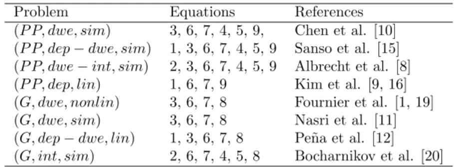
As mentioned in the introduction, research is active for optimizing energy in the field of railways and some attempts to classify the studied problems have been made. Xun et al. [17] proposed a classification of the methods used to solve the problems and Li et al. [18] listed without apparent classification some papers in the literature, detailing the decision variables or the algorithms used. To date, there is no formal classification of metro energy optimization problems. We propose a classification based on the previous timetable by a triple
(G/P P/CP, dep/dwe/int, sim/nonlin/lin)
denoting the choice of the objective function (G, P P or CP ), the decision variables (departure times, dwell times, interstation times or any combination
Problem Equations References (P P, dwe, sim) 3, 6, 7, 4, 5, 9, Chen et al. [10] (P P, dep − dwe, sim) 1, 3, 6, 7, 4, 5, 9 Sanso et al. [15] (P P, dwe − int, sim) 2, 3, 6, 7, 4, 5, 9 Albrecht et al. [8] (P P, dep, lin) 1, 6, 7, 9 Kim et al. [9, 16] (G, dwe, nonlin) 3, 6, 7, 8 Fournier et al. [1, 19] (G, dwe, sim) 3, 6, 7, 8 Nasri et al. [11] (G, dep − dwe, lin) 1, 3, 6, 7, 8 Pe˜na et al. [12] (G, int, sim) 2, 6, 7, 4, 5, 8 Bocharnikov et al. [20]
Table 1: Some metro timetabling energy optimization problems from the literature, classified by the problem triple they solve and the corresponding timetable equations.
of them) and the instant power demand evaluation (by an electrical simulator, a non-linear approximation or a linear approximation).
Table 1 classifies different problems studied in the literature using these triples. In this paper, we shall focus on the problems (G, dwe, lin) and (G, dwe, nonlin), that is, we focus on the problems of modifying solely the dwell times in order to minimize the global energy consumption of a metro line, evaluated using either a linear or a non-linear approximation. In this class of problems, the departure times dept, the interstation times intt,s, and the braking and acceleration phases
brkt,s and acct,s are given. The modification of the dwell times modifies the
arrivals at,s and departures dt,sin stations, and hence the auxiliary variables.
3.2. Complexity
First of all, one can remark that in absence of objective function, the time-table satisfiability problem is polynomial since all the equations of the timetime-table model are linear. Caprara in et al. showed in [21] that minimizing the deviation of a solution timetable comparing to an initial one to satisfy capacity or over-taking constraints is NP-hard. Serafini et al. showed in [22] that the problem of periodically scheduling trains with precedence constraints is NP-complete. Here we show the NP-hardness of several energy optimization timetable problems by polynomial reductions of SAT.
Theorem 1. The problem (G, dep, lin) is NP-hard.
Corollary 1. The problem (G, dep, nonlin) is NP-hard.
Corollary 2. The problem (G, dep − dwe − int, lin) is NP-hard.
The proofs are given in appendix. The idea of the proof of the first result is to construct a polynomial reduction of SAT to a particular (G, dep, lin) problem. A particular timetable is constructed such that all the acceleration phases can be synchronized with the periodic braking phases of only one special metro x0.
In this construction, it is possible to delay the departure time of each metro different from x0 by one time unit only. This ensures that one unit of energy is
saved at this time. A Boolean formula in conjunctive normal form (CNF) with c clauses is then satisfiable if and only if c units of energy can be saved in the timetable.
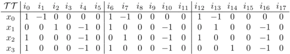
Example 1. Let us consider the SAT formula (x2∨ x3) ∧ (x1∨ ¬x2∨ x3) ∧
(¬x1∨ y). The constructed timetable contains four trips x0, x1, x2 and x3,
and is divided in three periods during which metro x0has the same behaviour.
For each braking phase of x0 occurring at times i1, i7 and i13, either x1, x2 or
x3 can be synchronized to save one energy unit. At each time unit, a metro is
either accelerating, consuming 1 energy unit, braking, producing 1 energy unit, coasting or dwelling, producing or consuming nothing. Each trip departure time can be delayed by one time unit. The formula is satisfiable if and only if for each braking phase of x0, one other metro can synchronize its acceleration phase
with it. The timetable with the energy consumed or produced by each metro at each time is shown in Table 2.
T T i0 i1 i2 i3 i4 i5 i6 i7 i8 i9 i10 i11 i12 i13 i14 i15 i16 i17
x0 1 −1 0 0 0 0 1 −1 0 0 0 0 1 −1 0 0 0 0
x1 0 0 1 0 −1 0 1 0 0 0 −1 0 0 1 0 0 −1 0
x2 1 0 0 0 −1 0 0 1 0 0 −1 0 1 0 0 0 −1 0
x3 1 0 0 0 −1 0 1 0 0 0 −1 0 0 0 1 0 −1 0
Table 2: Timetable energy problem encoding the satisfiability of (x2∨ x3) ∧ (x1∨ ¬x2∨ x3) ∧
(¬x1∨ x2). Each cell represents the power produced (-1) or consumed (1) by the trips xiat
each time. In this example, to save the 3 energy units produced by x0, and satisfy the SAT
formula in this encoding, it suffices to delay x3by one time unit since x1and x2already save
the 2 other energy units.
4. Instant Power Demand Model
The energy consumption of a metro line can be computed with an electrical simulator. The electrical circuit is composed of the N stations, the electrical substations (ESS) and the accelerating and braking trains at a given time.
The ESSs are electrical devices that convert the AC power provided by the electricity provider to DC power, directly usable by metros. We assume that they are not revertible, i.e. the regenerative braking can only be used by accelerating metros, and that they are directly connected to the stations. Part of the power provided by the ESSs is lost by Joule effects on the DC network.
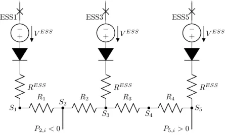
Each station is connected to the next one by a resistive cable. The braking metros are connected to the station to which they arrive and are modelled as an ideal power source. The accelerating metros are connected to the station from which they depart and are modelled as an ideal power sink. Figure 1 depicts the circuit associated to a small network with five stations, three ESSs, one braking metro and one accelerating metro.
ESS1 + − VESS RESS ESS3 + − VESS RESS ESS5 + − VESS RESS R1 R2 R3 R4 P2,i< 0 P5,i> 0 S1 S2 S3 S4 S5
Figure 1: Electrical circuit associated to a metro line with five stations at time i. It is composed of three electric sub-stations in S1, S3and S5, a braking metro arriving in S2 and
producing P2,i, and an accelerating metro departing from S5and consuming P5,i. The points
in the network are linked by resistive cables.
4.1. Network Parameters
The electrical properties of the metro line are fixed and given by the following set of parameters valid at any time:
• VESS
∈ R+ is the fixed voltage supplied by the ESSs to the line. Typical
values are 750V [10] or 1500V [12]. • RESS
∈ R+ is the value of the internal resistance of the ESSs.
• Rs ∈ R+ is the resistance of the electric cable of the metro network
be-tween the stations Ss and Ss+1, for 1 ≤ s ≤ N − 1. This is computed
using the linear resistance equation R = ρ.la , ρ being the resistivity of the third rail, a its section and l its length.
4.2. Timetable Parameters
Ps,i∈ R is the net power demand or production, involved by a metro, at time
i for every station Ss. This value is different from 0 only if there is effectively
a metro either braking or accelerating near the station at this particular time. These values are modified according to the acceleration and braking phases of the metros at each time point. We have
Ps,i
> 0 if metro accelerating near Ss
< 0 if metro braking near Ss
= 0 otherwise
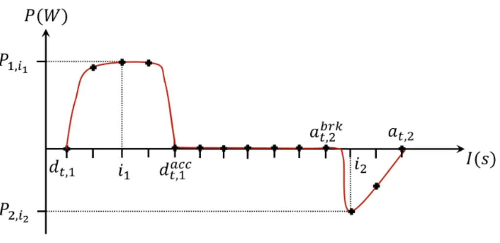
The precise power values are supposed to be known beforehand by direct mea-surement on the metro motors. Figure 2 illustrates the net power demand and production of a metro during an interstation run. In a typical example depicted in Figure 2, the parameters Ps,iare given by the power curve for each time point
i.
Figure 2: Net power demand and production curve as a function of real time for a metro accelerating and braking between two stations. The points on the curve represent the sampling over discrete time.
4.3. Electric Variables
The energy transfers are modelled by the following variables. By convention, all voltages are positive and the currents can be negative.
• vs,i ∈ R+ is the electric potential at station Ss, for 1 ≤ s ≤ N , at time
i ∈ I.
• is,i ∈ R is the current flowing through the cable between stations Ssand
Ss+1, for 1 ≤ s ≤ N − 1, at time i ∈ I.
• iESS
s,i ∈ R is the current flowing from the electrical substation connected
to the station Ss, for 1 ≤ s ≤ N , at time i ∈ I.
• iM ET
s,i ∈ R is the current flowing between the network and the metro
located in Ss, for 1 ≤ s ≤ N , at time i ∈ I.
4.4. Constraints and Instant Power Demand Value
The following equations constrain the current and voltage at each metro station. Ohm’s law gives
vs,i− vs+1,i= Rs.is,i 1 ≤ s ≤ N − 1, i ∈ I (11)
Kirchhoff’s current law gives
is,i+ is+1,i+ iESSs,i + iM ETs,i = 0 1 ≤ s ≤ N, i ∈ I (13)
The satisfaction of the instant power gives rise to a non-linear equation: Ps,i = vs,i.iM ETs,i 1 ≤ s ≤ N, i ∈ I (14)
It is worth remarking that the instant power demand of a metro line Pi is
not equal to the sum of the net instant power demands of the metrosPN
s=1Ps,i,
but to the power supplied by the electrical substations over the line to fulfil the metro power demands:
Pi= N
X
s=1
VESS. max(0, iESSs,i ) i ∈ I
This value represents the net power consumption of the metro line. The currents iESS
s flowing through each ESS can be negative, i.e. can flow backwards from
the line to the grid, but this negative power is not counted in the instant power consumption. Indeed, ESSs possess a rectifier that works as a diode and forces the current to flow only in one direction. In reality, if an electrical substation receives energy, typically when too many metros are braking and none is accel-erating, the energy is absorbed by resistors that are placed on the line or on the metros brakes.
5. Instant Power Demand Approximations
To simplify the evaluation of the power demand, some contributions in the literature have made the choice of directly computing the power transfers be-tween braking and accelerating metros instead of calculating voltages and inten-sities, and deducing the power demand from it [1, 9, 12, 16, 19]. We introduce in this section the notion of power flow network, which is a particular case of a generalized flow network, to model these power transfers. The idea is that set-ting the flow along the paths of the power flow network is an approximation of the power transfers between braking and accelerating metros, the flow arriving in the sink of the graph representing the power saved by regenerative braking reuse.
Both the electrical simulator and the power flow, model the fact that one accelerating metro can benefit from the regenerative energy of several braking metros and that one braking metro can feed several accelerating metros. The power flow approximation does not intend to reproduce exactly the electrical behaviour of the metro line but rather to give a fast evaluation of it for the optimization algorithm.
The distribution matrix ∆ is the matrix of distribution ratios ∆s,s0 = (P −
Ps0)/(Ps) ∈ [0, 1] between each stations Ssand Ss0, with 1 ≤ s0< s ≤ N , where
the negative net power production of a metro braking in station Ss, and P the
resulting power demand of the electrical network as computed by the electrical simulator. The distribution ratio represents the ratio of power a metro braking in station Ss effectively transfers to a metro accelerating in station Ss0. As
Ps0 ≥ P , a value of 1 means that the energy is fully transferred and a value of 0
means that the energy is completely lost in resistors as a consequence of Joule effects.
5.1. Power Flow Approximation
A generalized flow network is a finite directed graph G(V, E) given with capacities c(u, v) on edges in E and a flow f (u, v) ≤ c(u, v). The graph is given in addition with positive gains γ(u, v) such that, if a a flow f (u, v) is entering at vertex v, then γ(u, v).f (u, v) is going out from v:
X
v∈V |(u,v)∈E
γ(u, v)f (u, v) = X
v∈V |(v,u)∈E
f (v, u), (15)
Two vertices in V are distinguished, the source t which can produce flow and the sink t0 which can absorb flow.
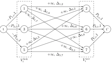
For each time i ∈ I, the power flow network is the generalized flow network defined by V = {t, t0} ∪ Vbrk i ∪ V acc i , Vibrk = {s, 1 ≤ s ≤ N |Ps,i< 0}, i ∈ I, Viacc= {s0, 1 ≤ s0 ≤ N |Ps0,i> 0}, i ∈ I, E = {(t, s)} ∪ {(s, s0)} ∪ {(s0, t0)} s ∈ Vibrk, s0 ∈ V acc i and c(t, s)i = Ps,i γ(t, s)i= 1 c(s, s0)i= +∞ γ(s, s0)i= ∆s,s0 c(s0, t0)i= Ps0,i γ(s0, t0)i= 1
The instant power demand approximation Pi can then be defined as:
Pi=
X
s0∈Vacc i
[c(s0, t0)i− f (s0, t0)i] (16)
Figure 3 shows an example of a power flow network modelling power transfers between 3 metros braking in stations S1, S3 and S5, and 3 metros accelerating
in stations S2, S6 and S7. The flows are attenuated between braking and
ac-celerating metros according to their distribution ratio ∆s,s0. The flows are not
bound and can be set freely between braking and accelerating metros. However, they are bound by the powers produced or demanded at the source or to the sink. The flows effectively arriving to the sink represent the regenerative power that has been saved, while the sum of the capacities’ edges arriving to the sink represent the total power demanded by the accelerating metros. Subtracting these two values gives an approximation of the instant power demand.
t 1 3 5 2 6 7 t’ Vbrk i V acc i −P 1,i ,1 −P3,i,1 − P 5,i,1 +∞, ∆1,2 +∞, ∆ 1,6 +∞ , ∆ 1,7 +∞, ∆ 3,2 +∞, ∆3,6 +∞, ∆ 3,7 +∞ , ∆5, 2 +∞, ∆5,6 +∞, ∆5,7 P 2,i,1 P6,i,1 P7,i ,1
Figure 3: Example of a generalized flow network. Flows are created by the source t and absorbed by the sink t0. The left hand side of the graph contains the vertices corresponding
to the braking metros, which are connected to the vertices corresponding to the accelerating metros on the right hand side. Each edge of the graph is characterized by a (capacity,gain) couple.
5.2. Power Flow Algorithm
According to the equation (16), the power demand equation of the power flow is equal to the capacities minus the flows directed to the sink. We have:
c(s0, t0)i= Ps0,i, s0∈ Viacc
and, according to the flow conservation equation (15)
f (s0, t0)i=
X
s∈Vbrk i
γ(s, s0)i.f (s, s0)i with γ(s, s0)i= ∆s,s0, s ∈ Vibrk, s0∈ Viacc
We can also reformulate the flow f (s, s0)i as the ratio of power transferred by
the metro braking at station Ss multiplied by the power Ps,i:
f (s, s0)i= −xs,s0,i.Ps,i, s ∈ Vibrk, s0∈ Viacc
The power transfer ratio xs,s0,i∈ [0, 1] is the ratio of the power Ps,i, with s ∈
Vibrk, transferred from the metro braking at station Ssto the metro accelerating
at station Ss0 such that xs,s0,i= −f (s, s0)i/Ps,i.
The following power flow algorithm computes the power transfer ratios by transferring the produced power of each braking metro in priority to the acceler-ating metro whose distribution ratio is maximum, until all the produced power is transferred. The algorithm returns the power transfer ratios xs,s0,i, either
when all braking metros have transferred their power or when all accelerating metros have their demand fulfilled:
Algorithm 1 Power transfer ratios computation at time i Require: Viacc, Vibrk, ∆s,s0, Ps,i
1: Initialize vector xs,s0,i← 0 2: while Vibrk 6= ∅ do 3: Choose randomly s ∈ Vbrk i 4: PIN IT ← Ps,i 5: while Ps,i < 0 do 6: if Vacc i 6= ∅ then 7: Choose s0 ∈ Vacc
i s.t. s0 = arg maxs0∈Vacc i (∆s,s0) 8: if −Ps,i.∆s,s0 > Ps0,ithen 9: xs,s0,i← (Ps0,i/∆s,s0)/PIN IT 10: Ps,i ← Ps,i+ Ps0,i/∆s,s0 11: Vacc i ← Viacc\{s0} 12: else 13: xs,s0,i← Ps,i/PIN IT 14: Ps0,i← Ps0,i+ Ps,i.∆s,s0 15: Ps,i ← 0 16: end if 17: else 18: Ps,i← 0 19: end if 20: end while 21: Vbrk i ← Vibrk\{s} 22: end while 23: return vector xs,s0,i
The instant power demand Pi can now be reformulated with the non-linear
equation: Pi= X s0∈Vacc i Ps0,i+ X s0∈Vacc i X s∈Vbrk i (Ps,i.xs,s0,i.∆s,s0), (17)
5.3. Linear Approximation for MILP
To avoid introducing too many variables in MILP, Pe˜na proposed in [12] a linear approximation of the power flow, which tends to maximize the overlapping times between acceleration and braking phases. The formulation of the power flow is simplified by authorizing only one single transfer between one braking metro and one accelerating metro. The objective function is then the sum, weighted by the distribution matrix, of the overlapping times of these transfers. The MILP model introduces two new variables to describe the overlaps be-tween metros :
• γt,s,t0,s0 ∈ {0, 1} is a boolean variable equal to one if the trip Tt, 1 ≤ t ≤ M
braking in station St(s), 2 ≤ s ≤ N , transfers its power to the trip
Tt0, 1 ≤ t0 ≤ M accelerating in St0(s0), 1 ≤ s0 ≤ N − 1. Otherwise it is
• Ot,s,t0,s0 ∈ R is the overlapping time between the braking phase of the trip
Tt, 1 ≤ t ≤ M at station St(s), 2 ≤ s ≤ N , and the acceleration phase of
the trip Tt0, 1 ≤ t0 ≤ M at station St0(s0), 1 ≤ s0≤ N − 1.
Constraint M X t=1 N X s=1 γt,s,t0,s0 ≤ 1 1 ≤ t0 ≤ M, 1 ≤ s0≤ N (18)
ensures that each accelerating metro receives the totality of the power of at most one braking metro, and constraint
M X t0=1 N X s0=1 γt,s,t0,s0 ≤ 1 1 ≤ t ≤ M, 1 ≤ s ≤ N (19)
ensures that each braking metro transfers the totality of its power to at most one accelerating metro, effectively modelling the fact that metros are only authorized to do one single pairing to transfer their power.
Constraint
Ot,s,t0,s0 ≤ brkt,s.γt,s,t0,s0 1 ≤ t < t0≤ M, 2 ≤ s ≤ N, 1 ≤ s0 ≤ N − 1 (20)
ensures that the overlapping time of a braking phase with an acceleration phase cannot be bigger than the braking phase time brkt,s.
Constraints
Ot,s,t0,s0 ≤ dacct0,s0− abrkt,s + m(1 − γt,s,t0,s0) (21)
Ot,s,t0,s0 ≤ at,s− dt0,s0+ m(1 − γt,s,t0,s0) (22)
1 ≤ t < t0≤ M, 2 ≤ s ≤ N, 1 ≤ s0≤ N − 1 ensure that the overlapping time is the minimum value of dacc
v,u− abrkt,s and at,s−
dv,uwhen γt,s,v,u= 1. The member m(1−γt,s,v,u), with m a big enough number,
ensures that O is never negative.
The MILP objective function used in [12]
maximize M X t=1 N X s=1 M X t0=1 N X s0=1 (Ot,s,t0,s0.∆s,s0) (23)
is the sum of all overlapping times of the timetables, weighted by the distribution matrix. The weights tend to synchronize braking and accelerations that are close to each other.
Concerning the size of the generated MILP instances, the model contains: • M2.N2 boolean variables γ, M2.N2 overlapping times variables O and
M.N dwell times variables dwe,
• 3M2.N2+ 2M.N MILP constraints (Equations 18, 19, 20, 21, 22) and
The MILP model thus introduces a quadratic number of variables and con-straints in the number of trips and stations. A pre-processing have been pro-posed in [12] to remove irrelevant constraints and variables. In particular, the number of overlapping variables Ot,s,t0,s0 to consider can be reduced by noticing
that two trips Ttand Tt0 such that dt,1> dt0,1+ trtt0 cannot overlap in any case.
However, this pre-processing is not sufficient to handle real data timetables as we will show in Section 8.
6. Greedy Heuristics Algorithm for (G, dwe, nonlin)
The idea of our heuristic algorithm is to shift the acceleration phases to synchronize them with braking phases and to recompute the non-linear objec-tive function to check for improvement. These local moves increase the power transfers between braking and accelerating metros, and possibly decrease the solution timetable global energy consumption.
6.1. Braking Phase Neighbourhood
The time neighbourhood of a braking phase N (at,s) is defined as the set
of acceleration phases that can overlap this braking phase within the given timetable tolerances. This means that every acceleration phase that may start before the end and finish after the beginning of a given braking phase, belongs to the neighbourhood of the latter:
N (at,s) = {dt0,s0|(t 6= t0) ∧ (dacct0,s0+ dwet0,s0 > abrkt,s) ∧ (dt0,s0+ dwet0,s0 < at,s)}
6.2. Acceleration Phase Shift Function
The acceleration phase shift function consists in modifying the departure time dt,sof a trip Ttat a station St(s) to make it correspond to the beginning
of the neighbour braking phase abrk
t0,s0 of a trip Tt0at station St0(s0), and by fixing
acct,s. The function considers the timetable constraints given by the bounds on
dwell times, trip times and headways. If the function cannot shift the departure time of the acceleration to the beginning of the braking phase due to tolerance constraints, it will shift it to the closest time which respects these constraints: Shift(dt,s, abrkt0,s0) =
(
dt,s:= max(abrkt0,s0, dt,s− max(dwet,s, trtt, hdwt,s)) if dt,s> abrkt0,s0
dt,s:= min(abrkt0,s0, dt,s− min(dwet,s, trtt, hdwt,s)) if dt,s< abrkt0,s0
Modifying dt,sconsists thus in modifying the duration of dwet,s, which will shift
6.3. Greedy Heuristics Optimization Algorithm
The algorithm comprehensively searches the acceleration phase shift that minimizes the objective function in the time neighbourhood of each braking phase,. All the braking phases are first sorted in chronological order and the acceleration phases are shifted for the earliest braking phases.
For each braking phase, the algorithm computes its time neighbourhood N (at,s), modifies each acceleration phase dt0,s0 by applying the shift function
Shift(dt0,s0, abrkt,s) and checks whether this shift is decreasing the objective
func-tion. If it does, the best current objective function and the best shift are up-dated.
When all the acceleration phases have been shifted and evaluated, the al-gorithm shifts the acceleration phase that minimizes the most the objective function, or does nothing if none of them decreases the objective function. This monotonic behaviour ensures that the algorithm will converge after some itera-tions and does not worsen the initial timetable. Once an acceleration phase is shifted, it is removed from the pool of neighbour phases and cannot be shifted any more for another braking phase. The following pseudo-code summarizes the greedy heuristics optimization algorithm:
Algorithm 2 Greedy heuristics optimization algorithm Require: T T
1: Sort at,s, 1 ≤ t ≤ M, 2 ≤ s ≤ N in chronological order
2: for all at,s do
3: Compute initial objective function GIN IT T T
4: Initialize best objective function GBEST
T T = GIN ITT T
5: Initialize best shift dBEST = 0
6: Compute N (at,s) 7: for all dt0,s0∈ N (at,s) do 8: dIN IT ← d t0,s0 9: Shift(dt0,s0, at,s) 10: Compute GT T 11: if GT T < GBESTT T then 12: GBESTT T ← GT T 13: dBEST ← dt0,s0 14: end if 15: dt0,s0 ← dIN IT 16: end for 17: if dBEST 6= 0 then 18: Shift(dBEST, a t,s) 19: end if 20: end for 21: return T T , GBEST T T
6.4. Incremental Computation of the Objective Function
Equation (17) shows that the instant power demand Pi is a function of the
net power demands and productions Ps,i, the power transfer ratios xs,s0,i and
the distribution matrix ∆s,s0. Since the distribution matrix is precomputed,
only the power transfers are modified by the optimization process.
In our dedicated heuristics, the objective function is re-evaluated every time an acceleration phase is shifted. Since a shift consists in modifying the dwell time of a specific trip at a specific station, many time instants remain with the exact same net power demand and production along the timetable. Let PiIN IT be the instant power demand at time i before a dwell time shift and Ps,iIN IT be the net power demands and productions at each station Ssat time i. After the
dwell time shift, only the instant power demands where the power demands and productions have changed need recomputing, as follows:
Pi=
(
PiIN IT if Ps,i= Ps,iIN IT ∀1 ≤ s ≤ N,
needs recomputation otherwise
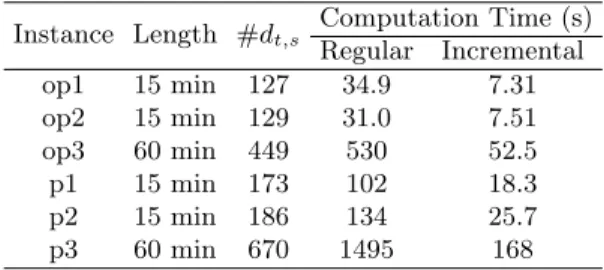
The incremental computation avoids recomputing known values, which increases the computation time of the algorithm by an order of magnitude as shown in Table 3 on six benchmark instances detailed in the following section.
Instance Length #dt,s Computation Time (s) Regular Incremental op1 15 min 127 34.9 7.31 op2 15 min 129 31.0 7.51 op3 60 min 449 530 52.5 p1 15 min 173 102 18.3 p2 15 min 186 134 25.7 p3 60 min 670 1495 168
Table 3: Computation time in seconds of one run of the greedy heuristics without and with incremental computation of the objective function. The two implementations are compared on the six benchmark instances described in Section 7 representing typical off-peak (op) or peak (p) hours timetables. The lengths of the timetable instances are either 15 or 60 minutes and the number of decision variables #dt,sare given.
6.5. Iterative Optimization
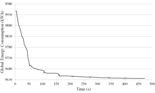
After one run of the algorithm, the optimized timetable can be utilized as input for a second run starting from the new solution. The optimization algorithm can thus be executed either once or iteratively until the iterative algorithm stops improving the objective function.
Figure 4 shows the minimization of the objective function using iterative optimization. It shows that the first run largely improves the timetable and that the following iterations lead to further improvements.
Figure 4: Evolution of the global energy consumption over computation time in seconds on a sample timetable during the iterative optimization process. The first cross represents the global energy consumption of the original timetable and the following ones the global energy consumption by iterating the greedy heuristics.
7. Performance Results Compared to MILP and CMA-ES
In this section, the greedy heuristics algorithm is compared to MILP and CMA-ES on six small size benchmark instances on which the three methods give solutions. Both the greedy heuristics and CMA-ES [13] are implemented in C++, and the MILP model is solved using CPLEX 12. The machine used for the experiments is a PC with an Intel Core i5 with 3GB of RAM.
For all the following results, a timeout of 1500 seconds was set. If not speci-fied otherwise, the objective function is computed using the electrical simulator described in section 4. The greedy heuristics used the incremental computation of the objective function and iterative optimization.
7.1. Benchmark Instances
The six timetables have been drawn from real data and represent relevant portions of the timetable, i.e. peak (p) and off-peak (op) parts of size of 15 minutes and one hour. These instances contain the initial parameters of the timetable (dIN IT
t,1 , dweIN IT, intIN IT and so on) as well as the tolerances, given
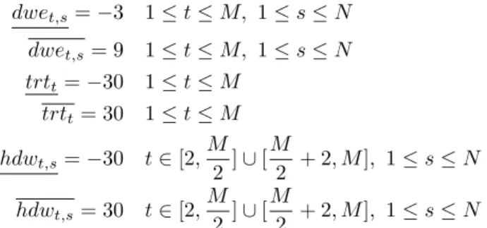
by the customer, on which variables can be modified and by how much. The tolerances on dwell times, trip times and headways are equal for all six instances. For the sake of simplicity, the tolerance values are given relatively to the initial timetable instance and dwet,s= −3 shall be read dwet,s− dweIN ITt,s = −3. The
departure times, the interstation times, the braking and acceleration phases lengths are fixed :
dwet,s= −3 1 ≤ t ≤ M, 1 ≤ s ≤ N dwet,s= 9 1 ≤ t ≤ M, 1 ≤ s ≤ N trtt= −30 1 ≤ t ≤ M trtt= 30 1 ≤ t ≤ M hdwt,s= −30 t ∈ [2, M 2 ] ∪ [ M 2 + 2, M ], 1 ≤ s ≤ N hdwt,s= 30 t ∈ [2, M 2 ] ∪ [ M 2 + 2, M ], 1 ≤ s ≤ N 7.2. Comparison with CMA-ES
Evolution strategies are stochastic search algorithms that try to minimize an arbitrary objective function called fitness function. The covariance matrix adaptation evolution strategy (CMA-ES) [13] applies to vectors of real-valued variables and arbitrary real-valued fitness functions. This algorithm is a multi-point method which at each iteration, samples the search space according to multivariate normal distributions, estimates its covariance matrix, determines a move to make in the most promising direction and updates the multivariate normal distributions for the variables. One important characteristic of CMA-ES compared to other meta-heuristics, is the limited number of parameters that need to be set, namely the initial standard deviation and the termination criteria. The other parameters are automatically adapted during the execution. The CMA-ES
In our experiments, we use the default value for the population size 4 + 3 log(#dt,s). The optimization is stopped after 10 iterations without
improve-ment of the objective function. The initial distribution has a default variance of (dwet,s− dwet,s)/7 for each trip at each station. A quadratic penalty function
is added to the objective function for each variable out of its domain, to enforce the algorithm to search solutions within the given tolerances.
Table 4 shows the results of CMA-ES against our heuristics. Due to its stochastic behaviour, CMA-ES has been run 100 times for each instance. The table compiles the average computation time, and both the average and best value found for the objective function over the 100 runs. The results show that the greedy heuristics performs better than the best run of CMA-ES on four of the six benchmark instances. On op1, our heuristics is better than the average result of CMA-ES but not than its best result. Finally, CMA-ES is slightly better than the greedy heuristics in average only for p3. The better performance of the heuristic algorithm is partly due to the incremental computation of the objective function, which cannot be implemented in CMA-ES since all solutions are sampled randomly.
7.3. Comparison with MILP
As shown in Table 5, CPLEX is able to prove the optimality on the four smallest instances and outperforms the greedy heuristics on the linear objective
Inst. Length #dt,s
Initial CMA-ES Greedy Heuristics Value Value
Time Value Time Average Best op1 15 min 127 2514 2401 2381 256 2394 45.6 op2 15 min 129 2516 2402 2388 223 2376 38.0 op3 60 min 449 9956 9724 9716 761 9556 648 p1 15 min 173 3433 3300 3285 503 3262 178 p2 15 min 186 3651 3516 3483 669 3442 291 p3 60 min 670 13067 12696 12675 1030 12713 1500
Table 4: Compared performance in computation time (Time in seconds) and energy consump-tion (Value in kW.h) between the average and best values found over 100 runs of CMA-ES and the greedy heuristics on six benchmark instances. The instances op represent an off-peak hour timetable and the instances p represent a peak hour timetable, both of either 15 minutes or 60 minutes long.
Instance Length #dt,s
Initial Greedy Heuristics MILP
Value Value Value Integrality gap op1 15 min 127 12.48 s 101.8 s 318.1 s optimal op2 15 min 129 11.48 s 159.1 s 351.6 s optimal op3 60 min 449 45.97 s 817.9 s 1637 s 10.62% p1 15 min 173 250.5 s 414.8 s 772.5 s optimal p2 15 min 186 279.1 s 533.8 s 835.8 s optimal p3 60 min 670 1019 s 1576 s 3003 s 20.44%
Table 5: Compared performances over the MILP objective function (Value in s) between CPLEX and the greedy heuristics on six benchmark instances. The MILP solutions are given with their integrality gap, optimal standing for 0%. The instances op represent an off-peak hour timetable and the instances p represent a peak hour timetable, both of either 15 minutes or 60 minutes long.
function (Equation 23). However, when comparing both optimization methods on the objective function computed with the electrical simulator (Table 6), our greedy heuristics performs better on five of the six instances.
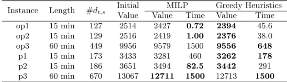
Instance Length #dt,s
Initial MILP Greedy Heuristics Value Value Time Value Time op1 15 min 127 2514 2427 0.72 2394 45.6 op2 15 min 129 2516 2419 1.00 2376 38.0 op3 60 min 449 9956 9579 1500 9556 648 p1 15 min 173 3433 3281 460 3262 178 p2 15 min 186 3651 3494 82.5 3442 291 p3 60 min 670 13067 12711 1500 12713 1500
Table 6: Compared performances in computation time (Time in seconds) and energy consump-tion (Value in kW.h) between MILP and the greedy heuristics on six benchmark instances. The instances op represent an off-peak hour timetable and the instances p represent a peak hour timetable, both of either 15 minutes or 60 minutes long.
This is due to the fact that the linear objective function is less accurate that the one used in the greedy heuristics (Equation 17). The main differences
between these two objective functions are that the MILP model is only able to pair one braking with one acceleration (Equations 18, 19), when the power flow objective function is able to dispatch dynamically to different braking and accelerations over time as described in Section 5.2. Thus eventhough our algo-rithm does not prove optimality, it better approximates the real behaviour of the electricity flows and leads to better solutions.
8. Performance Results on Real Data
Our greedy heuristics has also been applied on a major city metro line com-prising 16 stations for optimizing one full day timetable in two typical situations:
• a weekday timetable comprising 694 trips and 9585 dwell times, • a Sunday timetable comprising 556 trips and 7679 dwell times.
Both the C++ implementation of CMA-ES and the MILP resolution by CPLEX have failed to tame problems of this size. The MILP model contains, after its pre-processing, 230908 constraints and 165760 variables, whose 52872 are binary, and runs out of memory on CPLEX on a PC with an Intel Core i5 with 3GB of RAM.. The size of this instance is to relate with the size of the problem handled in [12] which was containing only 17850 constraints and 13860 variables, whose 4780 were binary. For CMA-ES, it fails at computing the global energy consumption of the initial population within 30 minutes. On the other hand, our greedy heuristics is able to compute a solution in 20 minutes. The tolerances on the dwell times, trip times and headways have been first set such that there is no visible change in the quality of service for the passengers. Their relatively small values are as follows:
dwet,s= −3 1 ≤ t ≤ M, 1 ≤ s ≤ N dwet,s= 3 1 ≤ t ≤ M, 1 ≤ s ≤ N trtt= −15 1 ≤ t ≤ M trtt= 15 1 ≤ t ≤ M hdwt,s= −15 t ∈ [2, M 2 ] ∪ [ M 2 + 2, M ], 1 ≤ s ≤ N hdwt,s= 15 t ∈ [2, M 2 ] ∪ [ M 2 + 2, M ], 1 ≤ s ≤ N
For the Sunday timetable, the trip times and headways tolerances have been enlarged to 20 seconds as follows:
trtt= −20 1 ≤ t ≤ M trtt= 20 1 ≤ t ≤ M hdwt,s= −20 t ∈ [2, M 2 ] ∪ [ M 2 + 2, M ], 1 ≤ s ≤ N hdwt,s= 20 t ∈ [2, M 2 ] ∪ [ M 2 + 2, M ], 1 ≤ s ≤ N
While the optimized timetable with regular tolerances is saving energy by 7.54%, the solution with increased tolerances can save up to 8.91%, increasing possibil-ities to synchronize phases better. Table 7 summarizes these results.
Instance Length #dt,s Initial CMA-ES MILP Greedy heuristics
weekday 1 day 9585 218294 - - 207052 (-5.15%) sunday15 1 day 7679 189953 - - 175638 (-7.54%) sunday20 1 day 7679 189953 - - 173036 (-8.91%)
Table 7: Compared performances in terms of energy consumption, given in kW.h, of CMA-ES, CPLEX and the greedy heuristics on three full size timetables. CMA-ES and CPLEX did not manage to output a solution. The ratios represent the energy savings compared to the initial timetable energy consumption.
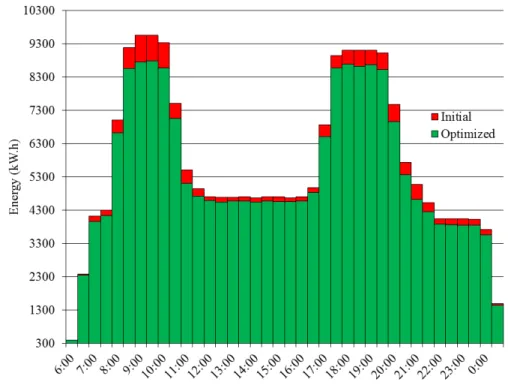
Figure 5: Weekday timetable between 6am and 1am: energy consumption by intervals of 30 minutes compared between the initial the timetable, in red, and timetable computed by the greedy heuristics in green.
Figures 5, 6 and 7 compare the initial and optimized timetable energy con-sumptions on three real data instances. For the weekday timetable, the two peak hour periods are clearly visible, from 8am to 11am and from 5pm to 9pm. It appears that more energy is saved during these hours. This is due to the fact that, according to the computed distribution matrix ∆s,s0, the energy transfers
Figure 6: Sunday timetable between 6am and 1am with a tolerance of 15 seconds on trips and headways: energy consumption by intervals of 30 minutes compared between the initial timetable, in red, and the timetable computed by the greedy heuristics in green.
density of metros on the line is higher during peak hours, it is thus possible to save more energy during these times. The extrapolation of these savings shows that the metro company could save 3.65 GW.h of electrical energy per year.
9. Conclusion
In this paper, we have proposed a generic mathematical model for metro energy optimization problems and a dedicated heuristics for solving the global energy consumption optimization problem by the sole modification of dwell times. This model has led us to a simple classification by triples of several similar problems of the literature, and to prove their NP-hardness.
We have shown that our heuristic algorithm for the problem (G, dwe, nonlin) performs better than the classical optimization methods used in the literature. On six small size benchmark instances on which MILP and CMA-ES could be run, we have shown that our heuristic algorithm computes better solutions. In particular for the MILP formulation, the results computed by CPLEX were of lesser quality due to the linear approximation of the objective function whereas our heuristics uses a non-linear power flow approximation. It was also shown to perform better than the state-of-the-art metaheuristic CMA-ES on these
Figure 7: Sunday timetable between 6am and 1am with a tolerance of 20 seconds on trips and headways: energy consumption by intervals of 30 minutes compared between the initial timetable, in red, and the timetable computed by the greedy heuristics in green.
instances thanks to the possibility of incrementally computing the objective function over iterations.
Furthermore, our dedicated heuristics was the only method able to solve a full day timetable of 7679 variables for the Sunday configuration and 9585 variables for the weekday configuration, decreasing the global energy consump-tion by 5.15% and 7.54%, and up to 8.91% by increasing the tolerances on the variables. These results show the applicability of this method in an industrial context.
References
[1] D. Fournier, F. Fages, and D. Mulard, “A greedy heuristic for optimizing metro regenerative energy usage,” in Proceedings of the second international conference on railway technology: research, development and maintenance (J. Pombo, ed.), (Ajaccio), Civil-Comp Press, 2014.
[2] I. E. Agency, “Energy balance for world.”
http://www.iea.org/stats/balancetable.asp?COUNTRY_CODE=29, 2009.
[3] T. O’Toole, “Environment report,” tech. rep., London Underground, 2006. [4] W. Rose and T. Rouse, “Sub-national electricity consumption statistics and household energy distribution analysis for 2010,” tech. rep., Department of Energy and Climate Change, Mar. 2012.
[5] J. Greatbanks, “Review of the discount for using regenerative braking,” AEA Technology, 2005.
[6] M.-Y. Ayad, S. Pierfederici, S. Ra¨el, and B. Davat, “Voltage regulated hybrid DC power source using supercapacitors as energy storage device,” Energy Conversion and Management 48, 2007.
[7] I. A. of Public Transport, “Reducing energy consumption in underground systems – an important contribution to protecting the environment.” 52nd International Congress of UITP, 1997.
[8] T. Albrecht, “Reducing power peaks and energy consumption in rail tran-sit systems by simultaneous metro running time control,” Computers in Railways IX, 2004.
[9] K. M. Kim, S.-M. Oh, and M. Han, “A mathematical approach for reducing the maximum traction energy: The case of Korean MRT trains,” IMECS 2010, Mar. 2010.
[10] J.-F. Chen, R.-L. Lin, and Y.-C. Liu, “Optimization of an MRT train schedule: Reducing maximum traction power by using genetic algorithms,” IEEE Transactions on power systems, vol. 20, pp. 1366–1372, Aug. 2005. [11] A. Nasri, M. F. Moghadam, and H. Mokhtari, “Timetable optimization
for maximum usage of regenerative energy of braking in electrical railway systems,” SPEEDAM 2010, 2010.
[12] M. Pe˜na, A. Fern´andez, A. P. Cucala, A. Ramos, and R. Pecharrom´an, “Optimal underground timetable design based on power flow for maxi-mizing the use of regenerative-braking energy,” Journal of Rail and Rapid Transit, vol. 226, pp. 397–408, July 2012.
[13] N. Hansen and A. Ostermeier, “Completely derandomized self-adaptation in evolution strategies,” Evolutionary Computation, vol. 9, no. 2, pp. 159– 195, 2001.
[14] ILOG, “V12.1: User’s manual for CPLEX,” International Business Ma-chines Corporation, vol. 46, no. 53, p. 157, 2009.
[15] B. Sans´o and P. Girard, “Trains scheduling desynchronization and power peak optimization in a subway system,” IEEE, 1995.
[16] K. Kim, K. Kim, and M. Han, “A model and approaches for synchronized energy saving in timetabling,” WCRR 2011, May 2011.
[17] J. Xun, X. Yang, B. Ning, T. Tang, and W. Wang, “Coordinated train control in a fully automatic operation system for reducing energy consump-tion,” Computers in Railways XIII, pp. 3–13, 2012.
[18] X. Li and H. K. Lo, “An energy-efficient scheduling and speed control ap-proach for metro rail operations,” Transportation Research Part B: Method-ological, vol. 64, no. 0, pp. 73–89, 2014.
[19] D. Fournier and D. Mulard, “Method and system for timetable optimiza-tion utilizing energy consumpoptimiza-tion factors,” Mar. 11 2014. US Patent App. 13/676,279.
[20] Y. Bocharnikov, A. Tobias, and C. Roberts, “Reduction of train and net energy consumption using genetic algorithms for trajectory optimisation,” in IET Conference on Railway Traction Systems, pp. 1–5, Apr. 2010. [21] A. Caprara, M. Fischetti, and P. Toth, “Modeling and solving the
train timetabling problem,” Operations Research, vol. 50, pp. 851–861, Sept./Oct. 2002.
[22] P. Serafini and W. Ukovich, “A mathematical model for periodic scheduling problems,” Society for Industrial and Applied Mathematics, vol. 2, pp. 550– 581, Nov. 1989.
Appendix A. NP-completeness proofs
Theorem 1. The problem (G, dep, lin) is NP-hard.
Proof 1. We show that there is a polynomial reduction of SAT to (G, dep, lin). Let X = {x1, ..., xm} be a set of m variables and ¬X = {¬x1, ..., ¬xm} be the
set of their negations. Let = φ be a Boolean formula in conjunctive normal form: φ = n ^ i=1 ci
where ci are clauses of the formW mi
j=1li,j with li,j∈ X ∪ ¬X.
Let us consider the discrete time domain I = {0, ..., 6n − 1}. Let T T be the metro timetable composed of a sequence of m + 1 trips T = (x0, x1, ..., xm)
running in the same direction, such that each trip xt∈ T crosses a sequence of
unique stations of length n + 1, and that the trips are :
• The trip x0cannot be shifted and is crossing stations every 6 time units,
departing from its first station at time i = 0: – d0,0= 0
– int0,s= 1 1 ≤ s ≤ n
– dwe0,s= 5 2 ≤ s ≤ n
Reminding the auxiliary variables equations: – the interstation time for a given trip,
intt,s= at,s+1− dt,s 0 ≤ t ≤ m, 1 ≤ s ≤ n, (A.1)
– the dwell time, or stopping time, in a station for a given trip, dwet,s= dt,s− at,s 0 ≤ t ≤ m, 2 ≤ s ≤ n, (A.2)
let us prove by induction that d0,s= 6(s − 1), 1 ≤ s ≤ n:
Basis: the statement holds for s = 1,
d0,1= 0 = 6(1 − 1)
Inductive step: if d0,s= 6(s − 1), then d0,s+1= 6s.
We can write
d0,s+1= d0,s+ a0,s+1− d0,s+ d0,s+1− a0,s+1
According to (A.1) and (A.2) we have:
d0,s+1= d0,s+ intt,s+ dwet,s+1
⇔ d0,s+1= 6(s − 1) + 1 + 5
We thus have:
d0,s = 6(s − 1), 1 ≤ s ≤ n (A.3)
a0,s = d0,s−1+ int0,s−1= 6(s − 2) + 1, 2 ≤ s ≤ n + 1 (A.4)
• Furthermore, the only possible shift applicable on trips xtin this timetable
is a delay of their departure time by 1 time unit, denoted δt∈ {0, 1}. The
trips xt with 1 ≤ t ≤ m are constructed according to the clauses ci of φ
as follows: – dt,1= δt+ 0 if xt∈ c1 1 if ¬xt∈ c1 2 otherwise 1 ≤ t ≤ m – intt,s= 4 if xt∈ cs 3 if ¬xt∈ cs 2 otherwise 1 ≤ t ≤ m, 1 ≤ s ≤ n – dwet,s= 2 if xt∈ cs 3 if ¬xt∈ cs 4 otherwise 1 ≤ t ≤ m, 2 ≤ s ≤ n
Like for x0, we prove by induction that
dt,s= 6(s − 1) + δt+ 0 if xt∈ cs 1 if ¬xt∈ cs 2 otherwise , 1 ≤ t ≤ m, 1 ≤ s ≤ n:
Basis: the statement holds for s = 1,
dt,1= δt+ 0 if xt∈ c1 1 if ¬xt∈ c1 2 otherwise = 6(1 − 1) + δt+ 0 if xt∈ c1 1 if ¬xt∈ c1 2 otherwise Inductive step: if dt,s= 6(s − 1) + δt+ 0 if xt∈ cs 1 if ¬xt∈ cs 2 otherwise , then dt,s+1= 6s + δt+ 0 if xt∈ cs+1 1 if ¬xt∈ cs+1 2 otherwise . We can write dt,s+1= dt,s+ at,s+1− dt,s+ dt,s+1− at,s+1
According to (A.1) and (A.2) we have: dt,s+1= dt,s+ intt,s+ dwet,s+1 ⇔ dt,s+1= 6(s − 1) + δt+ 0 + 4 if xt∈ cs 1 + 3 if ¬xt∈ cs 2 + 2 otherwise + 2 if xt∈ cs+1 3 if ¬xt∈ cs+1 4 otherwise ⇔ dt,s+1= 6(s − 1) + δt+ 4 + 2 0 if xt∈ cs+1 1 if ¬xt∈ cs+1 2 otherwise ⇔ dt,s+1= 6s + δt+ 0 if xt∈ cs+1 1 if ¬xt∈ cs+1 2 otherwise We thus have: dt,s= 6(s − 1) + δt+ 0 if xt∈ cs 1 if ¬xt∈ cs 2 otherwise 1 ≤ t ≤ m, 1 ≤ s ≤ n (A.5) at,s= dt,s−1+ intt,s−1= 6(s − 2) + δt+ 0 + 4 if xt∈ cs−1 1 + 3 if ¬xt∈ cs−1 2 + 2 otherwise ⇔ at,s= 6(s − 2) + δt+ 4, 1 ≤ t ≤ m, 2 ≤ s ≤ n + 1 (A.6)
Let the instant power demand function be
Pi= max(0, m
X
t=0
Pt,i) i ∈ I, (A.7)
where Pt,i∈ R is the power demand or production of the trip xtat time i. The
objective function is GT T. Let the trip acceleration and braking phases last
one time unit only. Each trip will demand one unit of power when departing from a station, and will produce one unit of power when arriving to a station. The rest of the time, each trip will not demand or produce any power. For all trips xt, the instant power demand or production Pt,i at time i can be written
as follows: Pt,i= 1 if ∃ 1 ≤ s ≤ n s.t. dt,s= i −1 if ∃ 2 ≤ s ≤ n + 1 s.t. at,s= i 0 otherwise (A.8)
Now let us prove that the global energy consumption is not modified by the powers produced by trips {x1, ..., xm} since they brake it when no trip is
accelerating. According to equations (A.6) and (A.8) we have:
Conversely and according to equations (A.3), (A.5) and (A.8), we have for all trips xt∈ T :
Pt,i= 1 if i = 6(s − 1) + (0 or 1 or 2 or 3), 0 ≤ t ≤ m, 1 ≤ s ≤ n (A.9)
Thus, there is no time where the braking of any trip in {x1, ..., xm} can be
synchronized with the acceleration of any trip in T :
@(i ∈ I, 1 ≤ t ≤ m, 0 ≤ t0 ≤ m) | Pt,i= −1 ∧ Pt0,i= 1
On the other hand, the braking phases of the trip x0 can be absorbed by
the acceleration phases of the other trips, optimizing the objective function. According to equations (A.4) and (A.8) we have:
P0,i= −1 if i = a0,s= 6(s − 2) + 1 2 ≤ s ≤ n + 1
Also according to equation (A.9), Pt,s = 1 if i = dt,s. To synchronize the
acceleration of the trip xtat station s with one braking of the trip x0we need:
a0,s+1= dt,s ⇔ 6(s + 1 − 2) + 1 = 6(s − 1) + δt+ 0 if xt∈ cs 1 if ¬xt∈ cs 2 otherwise ⇔ (δt= 0 ∧ ¬xt∈ cs) ∨ (δt= 1 ∧ xt∈ cs)
In other terms, the timetable is constructed such that for each trip xt and for
each station s we have:
• If the variable xt is in the clause cs, then the acceleration phase of xt
at station St(s) is synchronized with the braking phase of x0 at station
S0(s + 1) if and only if δt = 1. Thus setting δt= 1 is equivalent to say
that the variable xtis true, satisfying all clauses cscontaining it.
• If the variable ¬xt is in the clause cs, then the acceleration phase of xt
at station St(s) is synchronized with the braking phase of x0 at station
S0(s + 1) if and only if δt = 0. Thus setting δt= 0 is equivalent to say
that the variable ¬xtis true, satisfying all clauses cscontaining it.
• If neither the variable xt nor the variable ¬xt are in the clause cs, then
the acceleration phase of xtat station St(s) cannot be synchronized with
any of the braking phases of x0.
Every time one braking phase of x0 is synchronized with the acceleration
phase of one trip xt, one unit of power is saved. Given the period of time
I and the structure of the timetable, there is n power units that an optimal synchronization could save. Consequently, considering the decision problem of saving n power units, there is a timetable and a set of δt with 1 ≤ t ≤ m that
save n units of power if and only if the set of δ corresponds to a valuation that satisfies φ ; the n synchronizations corresponding to the n satisfied clauses.
Corollary 1. The problem (G, dep, nonlin) is NP-hard.
Proof 2. A problem is of class nonlin if it exists at least one equation which is non-linear. Modifying the equation (A.7) of the previous timetable into the non-linear equation ( Pi= max(0,P m t=0Pt,i) if 6l ≤ i ≤ 6l + 3 Pi= max(0,P m t=0P (2+1)k t,i ) if 6l + 4 ≤ i ≤ 6l + 5 ∀ 0 ≤ l ≤ n − 1
with k ∈ N, does not change the result of the objective function. Indeed, the timetable is constructed in such a way thatPm
t=0Pt,i ≤ 0, for all 6l + 4 ≤ i ≤
6l+5 and 0 ≤ l ≤ n−1. Thus, like for the previous timetable, Pi = 0, for all 6l+
4 ≤ i ≤ 6l + 5 and 0 ≤ l ≤ n − 1. Finally the problem becomes (G, dep, nonlin) without changing its resolution, thus the problem (G, dep, nonlin) is NP-hard.
Corollary 2. The problem (G, dep − dwe − int, lin) is NP-hard.
Proof 3. A problem is of class dwe if at least one dwell time can be modified. Likewise, a problem is of class int at least one interstation time can be modified. To get a problem (G, dep − dwe − int, lin), it suffices to add at the end of the timetable constructed in the proof of Theorem 1, one period of time where only x0 is running, and where its last dwell time and interstation time can be
modified.
Let us thus consider the metro timetable T T crossed by a sequence of m + 1 trips T = (x0, x1, ..., xm) crossing n + 1 stations each which encodes a Boolean
formula in CNF containing n clauses. To correctly encode the formula, the timetable should have a length of 6n − 1 time units. Let us add at the end of the timetable 4 additional time units where only x0 is crossing a new station
S0(n + 2) such that:
d0,n+1= 6n
a0,n+2= 6n + 1
Now, the last dwell time of x0 can be extended by one time unit, encoded in
δdwe= {0, 1},
dwe0,n+1= 5 + δdwe,
and the last interstation time of x0 can be extended by one time unit, encoded
in δint= {0, 1},
int0,n+1= 1 + δint
By adding these two tolerances, the problem (G, dep, lin), which encodes the SAT formula and which is NP-hard, has become a problem (G, dep − dwe − int, lin). Thus the problem (G, dep − dwe − int, lin) is NP-hard.