Design, analysis and control of an autonomous conveyance module for well exploration

Design, Analysis and Control of an Autonomous Conveyance

Module for Well Exploration

by

Pablo Valdivia y Alvarado

Bachelor of Science in Mechanical Engineering, 1999 Massachusetts Institute of Technology

submitted to the Department of Mechanical Engineering in partial fulfillment of the requirements for the degree of

Master of Science in Mechanical Engineering at the

Massachusetts Institute of Technology

February 2001

@2001

Pablo Valdivia y Alvarado. All rights reserved.

The author hereby grants to MIT permission to reproduce and to distribute publicly Paper and electronic copies of this thesis document in whole or in part.

signature of author... I certified by ... certified by ... accepted by... Chairm

Department f Mechanical Engineering February 2001

Samir A. Nayfeh Assistant Professor of Mechanical Engineering Thesis Supervisor

---' Bruce Boyle Program Manager, Schlumberger Doll-Research Thesis Sunervisor

Ain A. Sonin

BARKER

an, Department Committee on Graduate Students

MASSACHUSETTS tN TUTE OF TECHNOLoGy

Design, Analysis and Control of an Autonomous Conveyance

Module for Well Exploration

by

Pablo Valdivia y Alvarado

submitted to the Department of Mechanical Engineering on February, 2001 in partial fulfillment of the requirements for the degree of Master of Science in Mechanical Engineering

Abstract

Sophisticated sensors have been developed by the oil industry to provide accurate measurements of downhole physical characteristics. Traditionally, a module containing the sensors required for a given measurement job or "logging job" is lowered inside the well attached to the surface by a cable that provides power and support (wireline). The operation relies on gravity to convey the sensors to the section inside the well where measurements are needed. However, gravity does not help when the section to be attained is horizontal or at a relatively high inclination. As a preliminary response to this problem, several companies have developed tools called "tractors" which are motorized push-pull or wheeled vehicles that are attached to the front of the sensor modules and use the power provided by the wireline to pull the sensor pack inside the oil well. This preliminary solution seems to work appropriately for some horizontal and inclined wells provided the travel distance is not too large since the friction of the cable against the well casing becomes too large to overcome as its length increases. Considering that many horizontal and inclined wells in the market extend to lengths as large as 40,000 feet, considerable portions of live wells are still unattainable for measurements. Therefore, there is still a need for a solution that allows the complete exploration of horizontal wells.

Since the wireline or cable is the main problem when attempting to reach deep inside inclined and horizontal wells, this thesis proposes the development of an autonomous conveyance module for the sensors. However, an autonomous vehicle needs to carry its own power supply instead of relying on the continuous power available through the wireline. In addition, space constraints limit the amount of the supply (batteries) that can be carried downhole. Therefore, power efficiency is a first priority in the design of a module capable of traversing the required long travel distances. In general, traditional propulsion systems are very energy-inefficient since friction and heat dissipation, among others, take a good percentage of the energy used for motion. Consequently, an energy-efficient propulsion system is required in order to make the autonomous logging tool concept more feasible.

This thesis presents the theoretical analysis, design and control of a novel fluid propulsion system. The proposed solution uses the momentum of the fluid flow with a deployable, non-backdriveable mechanism in order to minimize battery usage and achieve controlled motions. A dynamical model of the physical behavior is presented and unknown model parameters are identified and validated through experimentation. The nonlinear dynamics of a module prototype are analyzed. Finally, using feedback linearization, and robust control techniques, appropriate control laws are derived in order to achieve satisfactory motion performance.

Thesis advisor: Dr. Samir A. Nayfeh

Title: Assistant Professor of Mechanical Engineering - MIT Company supervisor: Bruce Boyle

Acknowledgments

I would like to thank the Schlumberger-Doll Research Center for allowing me the time and resources to perform this research. My sincerest gratitude goes to Bruce Boyle, Dr. Raghu Mahdavan, and Dr. Olivier Sindt of the Conveyance Technologies program for their guidance and support, which made this work possible.

I would also like to thank my thesis supervisor, Professor Samir Nayfeh for carefully reading this manuscript and helping make it coherent.

Table of contents

LIST O F FIG U R ES... 6

C H A PTER 1: IN TR O D U C TIO N ... 7

1.1 BACKGROUND ... 7

1.2 PROBLEM STATEM ENT... 9

1.3 EFFICIENT PROPULSION SYSTEM ... 11

1.4 THESIS OVERVIEW ... 12

CHAPTER 2: MODULE EXTERNAL DYNAMICS...14

2.1 D YNAM IC BEHAVIOR M ODEL ... 14

2.2 LOSS COEFFICIENT M ODEL ... 20

CH A PTER 3: PR O TO TY PE D ESIG N ... 22 3.1 D ESIGN SPECIFICATIONS ... 22 3.1.1 Environm ent... 22 3.1.2 Geom etry ... 22 3.2 OBSTRUCTION M ECHANISM ... 23 3.2.1 Linkage M echanism ... 24 3.2.2 Petals ... 27 3.2.3 Linear Actuator... 28

3.3 POSITION FEEDBACK M ODULE ... 29

3.4 COM PLETE TOOL ... 31

CHAPTER 4: LOSS COEFFICIENT IDENTIFICATION... 32

4.1 EXPERIM ENTAL SETUP ... 32

4.1.1 Tool M odel... 32

4.1.2 Flowloop ... 33

4.1.3 Pump, Sensors and H ardware ... 34

4.2 EXPERIM ENTS... 38

4.3 RESULTS... 40

CHAPTER 5: OBSTRUCTION MECHANISM DYNAMICS... 45

5.1 KINEMATICS AND STATIC ANALYSIS OF LINKAGE MECHANISM ... 45

5.2 A CTUATOR DYNAM ICS ... 51

CH A PTER 6: M O D U LE C O N TR O L ... 55

6.1 PLANT M ODEL ... 55

6.2 O PEN LOOP STABILITY ANALYSIS ... 57

6.3 CONTROL IM PLEM ENTATION AND OBJECTIVES ... 62

6.3.1 Input-O utput linearization ... 63

6.3.2 Robust Control... 66

6.4 PROTOTYPE H ARDW ARE IM PLEM ENTATION ... 73

CHAPTER 7: CONCLUSIONS AND FUTURE WORK ... 76

7.1 SUM M ARY OF CONTRIBUTIONS... 76

7.2 FUTURE W ORK... 77

REFERE N C E S ... 78

APPENDIX B: COMPOSITE PETALS FABRICATION... 111

APPENDIX C: SIMULATION ALGORITHMS ... 115

List of figures

FIGURE 1.1: W IRELINE W ELL LOGGING ... 8

FIGURE 2.1: FLUID FLOW OBSTRUCTION CONCEPT. ... 14

FIGURE 3.1: LINEAR ACTUATOR DRIVEN "UMBRELLA" MECHANISM. ... 24

FIGURE 3.2: LEGO PROTOTYPE OF UMBRELLA MECHANISM ... 25

FIGURE 3.3: LINKAGE MECHANISM CONCEPT DRAWING. ... 26

FIGURE 3.4: FINAL PROTOTYPE LINKAGE MECHANISM WITH PETALS ATTACHED. ... 27

FIGURE 3.5: C OM POSITE PETALS ... 28

FIGURE 3.6: LINEAR ACTUATOR ATTACHED TO UMBRELLA MODULE. ... 29

FIGURE 3.7: POSITION FEEDBACK M ODULE. ... 30

FIGURE 3.8: COMPLETE TOOL ARRANGEMENT. ... 31

FIGURE 4.1: TOOL MODEL CONCEPT DRAWING... 32

FIGURE 4.2: ALUMINUM CONES USED TO TEST THE "UMBRELLA" SHAPE PROPERTIES... 33

FIGURE 4.3: DIAGRAM OF FLOWLOOP SETUP (NOT TO SCALE). ... 34

FIGURE 4.4: CENTRIFUGAL PUMP MOUNTED ON ITS INERTIAL BASE. ... 34

FIGURE 4.5: ELECTROMAGNETIC FLOWMETER... 35

FIGURE 4.6: LOAD CELL MOUNTED ON TOP OF T-JUNCTION ... 36

FIGURE 4.7: FLU ID R ESERVO IR. ... 37

FIGURE 4.8: D ATA ACQUISITION EQUIPMENT. ... 37

FIGURE 4.9: FRONT VIEW OF FLOW LOOP... 38

FIGURE 4.10: MODEL BEING SUBMERGED INSIDE THE FLOWLOOP. ... 39

FIGURE 4.11: CLOSE UP OF MODEL INSIDE THE LOOP... 39

TABLE 4.1: CHARACTERISTICS OF CONICAL FIXTURES. ... 41

FIGURE 4.12: EXPERIMENTAL RESULTS FOR CONE 1. ... 42

FIGURE 4.13: EXPERIMENTAL RESULTS FOR CONE 2. ... 42

FIGURE 4.14: COMPARISON OF CONE'S BEHAVIOR ... 43

FIGURE 4.15: VALIDATION OF LOSS COEFFICIENT MODEL USING EXPERIMENTAL DATA FROM CONE 3. ... 44

FIGURE 4.16: VALIDATION OF LOSS COEFFICIENT MODEL USING EXPERIMENTAL DATA FROM CONE 4. ... 44

FIGURE 5.1: UM BRE LLA-ACTUATOR MECHANISM... 45

FIGURE 5.2: L-SH APED LINKAGE FBD ... 46

FIGURE 5.3: INTERM EDIATE LINKAGE FBD ... 47

FIGURE 5.4: ACTUATOR CONNECTION BASE FBD... 47

FIGURE 5.5: L IN KA G E SYSTEM . ... 48

FIGURE 5.6: LINEAR ACTUATOR COMPONENTS... 51

FIGURE 6.1: OPEN LOOP SYSTEM BEHAVIOR WITH CONSTANT DISTURBANCE... 68

FIGURE 6.2: TRACKING ERRORS AND CONTROL ACTIVITY WHEN MAINTAINING CONSTANT POSITION,... 69

AGAINST A CONSTANT DISTURBANCE. ... 69

FIGURE 6.3: TRACKING ERRORS AND CONTROL ACTIVITY WHEN MAINTAINING CONSTANT VELOCITY, ... 70

AGAINST A CONSTANT DISTURBANCE. ... 70

FIGURE 6.4: OPEN LOOP SYSTEM BEHAVIOR WITH TIME VARYING DISTURBANCE... 71

FIGURE 6.5: TRACKING ERRORS AND CONTROL ACTIVITY WHEN MAINTAINING CONSTANT POSITION,... 72

AGAINST A TIM E VARYING DISTURBANCE... 72

FIGURE 6.6: TRACKING ERRORS AND CONTROL ACTIVITY WHEN MAINTAINING CONSTANT VELOCITY, ... 72

AGAINST A TIM E VARYING DISTURBANCE... 72

FIGURE 6.7: PROPULSION MODULE HARDWARE ARCHITECTURE... 75

F IG UR E B . 1: P ETA L L AY ERS... 111

FIGURE B .2: E PO XY APPLICATION ... 1 12 FIGURE B.3: FIBER LAYERS ARE PUT INTO A VACUUM OVEN... 113

FIGURE B.4: FIBER LAYERS CLAMPED ON DIES ARE PLACED INSIDE AN OVEN. ... 113

Chapter 1: Introduction

1.1 Background

In the oil industry, production logging is the process of evaluating a well by determining the properties of its rock formations and the existent fluids (e.g. oil, water, and gas). A sonde, which can contain one or several sensors, is attached to the end of a cable or "wireline" and lowered inside the well as shown in figure 1.1. Electrical, acoustical and radioactive properties of the formations and their fluids are measured by remote sensing as the sonde is brought back up the hole at a constant speed. These measurements

provide the operator of the well with detailed information on the nature and behavior of fluids in the drilled hole or "borehole" during production or injection.

Production logging emerged in the 1930s with the introduction of the temperature log. By the late

1950s and early 1960s, many different production logging techniques were being used. The problem was

that each technique required a separate trip into the well. The 1970s saw tools that combined several measurement techniques, meaning a more efficient single run in the well. Improvements have continued through the 1980s to the present day with better sensors and deployment methods. The latest tools use new technologies to completely measure production data around the borehole. Many sensors can be combined into one tool and recorded simultaneously to measure fluid entries and exits, standing liquid levels, bottom hole flowing and shut-in pressures, pressure losses in the tubing, and the integrity of the gravel pack and hardware assemblies. Since the measurements are made simultaneously, their correlation is less affected by any well instability that might cause downhole conditions to vary over a period of time. The sensors available for logging include: thermometers, fluid sampling, flowmeters, manometers, noise probes, calipers, radioactive tracers, water flow logging, gravel pack logging, phase velocity logging, three-phase holdup, and down hole video cameras. Finally, a production logging tool (PLT) string will always include a depth control device since the correlation between the measurements and the depth at which they were taken is crucial for their clear interpretation.

Wireline Truck

Logging Tools

Figure 1.1: Wireline well logging

F

Well

Downhole tools must also withstand the extreme well environment. Temperatures inside the borehole can range between -40 and 200 degrees Celsius, and the pressures vary from 0 to 15000 Psi (gage). In addition, flow regimes can be single or multiphase and with widely ranging densities and viscosities. Typical wells extend to depths of 10000 feet (vertically), and some horizontal or inclined branches detach at various heights. These branches can in turn extend for several thousand feet. Finally, the inside diameter of the well casing generally ranges between 1.2 and 6.2 inches and some obstacles like joints, tubing nipples, perforations, distorted or partially collapsed tubing, and some sections with sand and gravel deposits are also typically found in the borehole [17]. Obviously, these conditions vary among wells, nevertheless logging tools must be designed to withstand, fit and navigate through most of them so they can service the majority of the market.

1.2 Problem Statement

Logging measurements are a crucial part of the production process of a well because of the insight they give. Basically, their information helps determine the economic viability of exploiting a well. As explained in the previous section, PLTs are attached to the wireline and then lowered inside the well to attain the depths at which measurements are required. When the well to be logged is vertical, or nearly vertical, the weight of the tools and the weight of the cable are sufficient to overcome any friction against the borehole wall, as well as any resistance due to fluid drag. Therefore, it is relatively easy to lower any type of tool inside wells with inclinations between 0 and 75 degrees relative to the vertical axis. However, in recent years there has been a shift in the industry and more and more wells are drilled wherein at least a portion of the borehole is horizontal or at a large angle relative to the vertical axis. In this type of well gravity does not help convey the tools attached to the wireline. Hence, conveying PLTs to the inclined parts of the well becomes more complicated if not impossible. In this case, a solution is to push the logging tools with a thick-walled steel pipe denominated "drill string"used in rotary drilling [17]. However, this process is time consuming, expensive, and can damage the logging tools as well. Alternatively, some companies have developed wheeled or push-pull propulsion modules, commonly denominated as "tractors". These modules are attached to the front of the sensor pack, and powered by the wireline. Hence, they help convey the sensor pack inside the borehole when gravity can not be used. Even so, after a couple of thousand feet of travel in a fairly inclined or horizontal part of the well the friction between the wireline cable and the well casing becomes too large to overcome. Hence, deep sections of these wells are still impossible to attain with these methods.

For an optimal logging job, assuming the sensor pack works properly, there are essentially two functional requirements. First, good motion control of the logging tool has to be achieved. The logging tool has to be able to attain any point inside the well, which translates into having control over its depth. Also, to perform good measurements the logging tool must have good control of its displacement rate as well. This motion control must be achieved regardless of the state of the downhole environment. Secondly, the PLT should not get stuck easily inside the well since this would jeopardize production.

Hence, different design parameters should be used to address the problem of moving the logging tools inside the well. An alternative method of conveyance should address any functional requirements not satisfied by the current methods and perform at least at a comparable level in settings were previous methods worked. A propulsion system, integrated to the PLT string, provides motion independently of the inclination of the well. Furthermore, in this modality a cable is not needed to control the rate of motion of the tools, and actually restricts the motion by causing friction problems. Hence, the use of the wireline services can be avoided, and an "autonomous logging tool" can be used to navigate inside the wells and perform the required measurements without being attached to the surface. However, by eliminating the wireline one also eliminates its advantages. From a technical prospective there are three advantages when using a wireline in the conveyance of tools. First, additional energy can be provided from the surface to downhole tools whenever needed. Secondly, in the event of an accident were the tools become jammed inside the well, the wireline can be used to pull them free. Finally, in vertical wells, the wireline is used to control the rate at which the PLTs move.

Hence, for an autonomous tool to be practical it must overcome three problems: power consumption, retrieval from downhole, and motion control. The problem of retrieval of tools from downhole, commonly referred as fishing, is not new in the industry and some techniques for this have been refined. Essentially, the process consists of using a cable, not necessarily the wireline, to catch and pull free the trapped tools. Presently, in most downhole tools, the housing enclosing the connectors at the downhole end of the wireline has a neck or reduced diameter designed to be caught securely during "fishing" operations. This feature can also be incorporated into tools not using the wireline. Therefore, we will center our study only to the problems of power consumption and motion control.

Downhole tools are electromechanical devices, hence an autonomous version requires batteries to supply power. However, current battery technology is not advanced enough to provide sufficient energy for a round trip inside a well when using traditional propulsion systems. Even lithium batteries, which have the highest energy density among all batteries, can not provide as much energy per volume as gasoline or other fuels [6]. Therefore, power supplies using batteries need to be recharged often, which is a wide spread problem in mobile robotics. Consequently, power requirements need to be kept at minimum if single runs inside the wellbore are to be made without the necessity of recharging the power supply in the middle of a

"mission". Failing to do so would require the implementation of some sort of recharging stations along the well casing, so the autonomous module can complete a trip, bringing more complexity to the project.

Wheeled devises, propellers, and inchworm mechanisms are all propulsion devices that can be used effectively to achieve motion inside a pipe filled with fluids. However, the problem when using these propulsion mechanisms is their low energy-to-motion performance ratios. Among all, wheeled mechanisms are the most efficient if designed correctly. Nevertheless, not enough energy can be carried on board a reasonably seized autonomous device to achieve a round trip since distances inside a well are prohibitive. A possible solution, whose implementation is the subject of this thesis, is the use of the flow existent inside a well as means of an alternative propulsion force. A design is presented in which the fluid momentum is used to achieve motion with minimal internal power consumption. Such a device can be combined with traditional wheeled modules to achieve the propulsion necessary for an autonomous logging tool, providing motion control with an alternative low-power-consumption module.

1.3 Efficient propulsion system

For our purposes, let us define a "propulsion mechanism" to be a device that achieves the displacement of the piece of equipment in which it is contained. In our case, the motion needs to be achieved through fluids. The main problem with traditional propulsion mechanisms is that a good percentage of the energy that should be devoted to motion is actually lost through friction and heat dissipation (no motor or actuator is %100 efficient). In addition, mechanisms such as wheeled devices or propellers require constant activity of the propulsion apparatus to achieve motion, thereby consuming energy all the time. Given our constraints, an ideal propulsion mechanism would be one that can achieve controlled motions using very little or no energy.

Under normal operating conditions, only four forces act on objects inside an oil well: drag, buoyancy, friction, and gravity. The drag is caused by the existent fluid flow inside the well and it acts in the direction of flow. This flow could be of single or multiphase nature (e.g. pure oil, water or combinations with gas). The buoyancy is the effect of the difference in densities between the tool string and its environment. Frictional forces arise because in order to perform accurate measurements, logging tools have to be aligned with the wellbore axis thus, spring loaded devices called centralizers are always in contact with the

borehole. Also, viscous friction is due to fluid interaction with the tools. Finally, downhole tools are usually made out of high strength alloys in order to withstand the harsh environments of wells, and their lengths together with their weights can vary a lot.

Among these forces, the weight of the tools is usually the largest because logging tools are in general streamlined and open to the fluid environment to keep drag forces and buoyancy minimal. Additionally, the centralizing parts that press against the well casing have wheeled joints so friction is minimized. However, given the flow ranges present in the wellbore, if drag effects are maximized, they can eventually overcome the weight of the tools plus any friction with the wellbore, and "lift" the entire tool string. If a device is designed so as to control accurately the magnitude of drag forces exerted on the tool string then it will be possible to achieve a fairly accurate motion control.

In principle, a mechanism that controls the drag should consume less power than traditional propulsion systems since it does not need to overcome external forces at all times, like wheeled devices, but instead uses their momentum to its advantage. As an analogy, one can think of the difference of energy consumption between a parachute and an elevator: both mechanisms can bring objects safely to ground, however the parachute does not need any energy to operate except for the one used to deploy it. If we can control this mechanism such as to accomplish precise motions and velocities, trajectory control could be achieved with minimal use of energy in comparison to traditional propulsion devices.

Therefore, we want to design and control a mechanism that uses the momentum provided by fluid flow to achieve axial displacement inside well pipes. If we want to use the momentum provided by fluid flow, the simplest design concept is to create an obstruction in the pipe thereby generating a pressure differential across the obstruction. The force resulting from that pressure differential can then be used for motion control.

1.4 Thesis overview

The objective of this research is to solve the problem of designing and controlling an obstruction mechanism for an autonomous logging tool. This mechanism should achieve "controlled motions" up and down stream inside segments of oil wells with low power consumption. In Chapter 2, we provide a study of the downhole dynamic behavior of a tool with a generic obstruction mechanism. Key physical relationships

are presented relating the geometry of the obstruction to its performance as part of the propulsion mechanism. The main result of this section is a generalized equation of motion for centralized objects moving inside pipe sections that we use for simulations (e.g. external dynamics). In Chapter 3, we describe the mechanical design of the proposed prototype, which is the main contribution of this thesis. Based on insights from the dynamic behavior analysis, an obstruction shape is chosen and a mechanism that implements it is devised. The methodology for material and component selection is explained accordingly. In Chapter 4, we explain how the unknown model parameters, for the obstruction shape chosen, are identified through experimentation. The results are presented along with a description of the experimental procedure. The dynamics of the electromechanical propulsion module apparatus are presented in Chapter 5. In Chapter 6, the results from the analysis of the obstruction apparatus dynamics and the module external dynamics are combined into a complete model of the module behavior, which is of nonlinear nature. The state representation of this model is used for nonlinear control design. An analysis of the module stability in open and closed loop is presented along with an appropriate implementation of control laws. The use of feedback linearization and robust control techniques for the implementation of the control laws is explained in detail, and simulations of the module trajectory tracking are presented. The hardware architecture required for the module is also laid out. Finally, in Chapter 7 we present the conclusions, a summary of the contributions of this thesis, and recommended future work. All the machine drawings, some component fabrication methodologies, the control algorithms used for the simulations, and some mathematical background for the control analysis can be found in appendices A, B, C, and D respectively.

Chapter 2: Module External Dynamics

2.1 Dynamic behavior model

The simplest way to exploit the momentum provided by fluid flow is to create an obstruction in the pipe flow. Figure 2.1 is a diagram of the basic physical elements involved in the implementation of an

obstruction in the fluid flow inside a well. Fluid arrives at the obstruction with an average velocity v1, and

creates a pressure P that acts underneath the obstruction. The average velocity of the fluid as it leaves the

obstruction is v2, and a pressure

P2

acts on top of the obstruction. The radius of the tool is shown as

R,

the radius of the obstruction is

R

2, and the radius of the pipe is denoted as R .

<

... _->R

R

R

2

R

F

i

2

P

₂

r---P

1

"PtAL

AkZ

*711;

V 2 --- 1 c.v.I

r1

Vi

The obstruction behavior can be analyzed as a pipe flow problem. For the fluid dynamics analysis we use a cylindrical control volume underneath the obstruction, of fixed length 1 and radius R , attached to the

tool as it moves. Let us define the area A, to be the area between the well I.D and the tool

O.D,

and the

area A2 to be the area between the well I.D and the obstruction O.D, hence assuming that both the tool and

the obstruction used have circular projected areas,

A1 =g(R2 - R2)

(2.1)

A2 =c(R 2

-

R22)

(2.2) This assumption is quite normal for downhole hardware since the medium itself (the well casing) is of cylindrical nature thus in order to achieve good mobility most hardware is designed in this fashion.

The Reynolds Transport Theorem applied to the conservation of mass inside our control volume can be written as:

d {JJpdV}+J p(e-n h)dA = 0

CY C.S

where Vrel = Vabsolute - , and p is the density of the fluid media. Assuming the fluid inside the well is

incompressible, the above equation simplifies to:

(Aie),, = I (AT )Out

The tool and the control volume travel at a velocity

vc.j

= ± (positive upward). The absolute velocity

of the fluid coming into the control volume is (Vabsolute

)n

=

vI

, therefore the relative velocity of the fluid coming into the C.V. is (Vrein = VI - i. Alternatively, let us define the relative velocity leaving the

control volume as (Vre )ou= V - ZVre2 .Therefore, from the conservation of mass across the control

volume we find that the relative velocity of the fluid coming out of the obstruction can be expressed in terms of the rest of the variables as:

(v1

-

Z)A1 Vrel 2 -(I _{V 2)A}

2- A₂

(2.3)

We now apply the Reynolds Transport Theorem (RTT) to the conservation of linear momentum on our control volume and get:

dt

dt

JipdV

+

~ie

-r dS = X F + FB

C.V C.S

The forces,

F,

exerted on the control surface are mainly the pressure and viscous forces, and the only

force, FB, acting at the control volume center is the gravity force. We purposely neglect any viscous

stresses on the control volume since their magnitude is very small compared to the forces due to pressure. Therefore, for our accelerating control volume, the conservation of momentum can be written as,

dJJvez pdV

- pv el 2

Al

+ PVre 22 A2 =

APzcR

2 _{- ( + gp,2}

1

L,

-

pizR

12

L,

+ p/A)

where

p,

and

Lt

are the density and length of the tool providing the obstruction, AP is the pressure

differential across the obstruction ( AP = P - P2 ), g is the gravitational acceleration, and 2 is the

acceleration of the control volume. The term vrelZ represents the average z-component of velocity of all the

fluid, relative to the control volume [3][4][5]. Thus,

d

dV

- 1 VreIZpdV = pAl eIZ = pA l( z -4Z)

dt C. V dt

where 'tz is the average absolute acceleration of the fluid in the control volume. Solving the Navier-Stokes

equation for one-dimensional incompressible flow, and then differentiating the result would yield an

approximation of the actual value for the fluid acceleration. However, we can simply neglect z I If the

velocity of the fluid flow across the control volume changes smoothly, then our assumption is justifiable. Otherwise, the result of this assumption would be to simply underestimate the momentum of the fluid in the control volume. The impact in the accuracy of our model will not be substantial unless the mass of the fluid in the control volume is significantly bigger than the mass of the tool whish is not the case here. The

density of downhole tools is generally bigger than that of the fluids (oil and gas mixtures). If we let

M'=

prR

1

L,

-

pfrR2

L,,

denote the equivalent mass of the module (mass minus buoyant effects) we

get

m' = PVre 2

A

1

-

Vre22

A

₂

+ APirR

2

- pgAl -m'g

(2.4) Equation 2.4 describes the motion of the module inside a pipe. In order to solve it we need to know the

values of the fluid absolute inlet velocity v1, density

p,

and the differential pressure

AP.

The values of

the fluid velocity and density are a priori unknown but bounded. Typical flow velocities inside an oil well

are between 0.1 and 10 (m / s), and the densities of the medium range between 500 and 1500 (kg /

M

3_).

We show in Chapter 6 that control laws can handle parametric uncertainties in the model provided that we have bounds for them. However, the value of the differential pressure is harder to bound directly since it depends on the obstruction effects. Hence it is necessary to attempt an approximation. If we apply the RTT to consider the conservation of energy in our accelerating control volume we would get an equation similar to 2.4. However, a simpler view can provide a straightforward and useful relation. At steady state we need not include the effects of the control volume acceleration in the energy equation thus we can use the simpler relation,

+JffepdV

+ Jfepvre,.

dS

=

Q

-Z

dC. V C.S

where

e

is the total energy of the control volume per unit mass,

Q

is the heat supplied to the system by the surroundings (we will assume none) and IW is the sum of all the "shaft" work done by the system.

Furthermore, for steady flow along a streamline between points

1

and 2 the above equation can be simplified to the extended Bernoulli equation (or mechanical energy equation):

2

r

2

w, - --

ghl,

=

(

2

+ gz

- (V' + gz

f _{I 2 /)2 2}

where

+w

is the work input/output of the moving fluid due to pumps or turbines (in this case none), and

ghrs, is an energy dissipation term due to heat losses, frictional losses, and form losses. Evaluating the

above equation for our control volume we get:

P + p(v - )2 + pgz, = P₂ +- pv _{2 +Pz 2 I p(v - j)2 K,}

2

2

2

with z2 and z, being the heights of the top and bottom of the control volume inside the pipe with respect to

an inertial reference frame. The loss coefficient

K,

is associated with the obstruction in the pipe and is

defined as: (K,)I =

(h,

2,) . Rearranging the terms of the above equation we get an expression for

vx

the pressure differential across the obstruction:

AP=- pv2 ±pgl

+-

p(v, - )2(K,

-1)

2

2

(2.5)

Equation 2.5 is clearly only an approximation of the existent differential pressure since we are neglecting the effects of the accelerating control volume, and the flow around the obstruction will certainly not be steady. Nevertheless, equation 2.5 allows us to provide a model structure for AP with parameters for which

we have bounds such as v,, and

p.

The loss coefficient K, is unknown, and its value is highly dependent

on the shape of the obstruction. Therefore,

K,

should be experimentally identified for the obstruction

profile we choose in our design.

Combining equations 2.3, 2.4, and 2.5 we can obtain the equation of motion of the obstruction tool inside the well. Factoring the terms we can write the equation of motion as:

Z =

a2z2 +alz+ao

where: 2 A2 2 a2=p

K,)R

+A1 +

A

R 2 nt 2 A2 2A2 a1 2 (Kl -1)rcR 2 A 2 2 J n a,

= -2v~p (,-1;R2+A - A,2+

A2

2 ;TR 2 m

2

A2

2A2

r2 (K, 13R2 A A 22 a0 = 2 p

-

₂

+

-A,

+

A

22

pglzR

- g mnR '+ A2

2

A2

Equation 2.6 is a nonlinear second order differential equation best known as the Riccati equation.

Equation 2.6 can be solved using a change of variables such as: y = i, which reduces the order of the

equation that can now be written as:

dy

dt

22 a2y2 + a~y+ a0

and can be solved by integration. If we take S, and s2 to be the roots of a2y2 + aly + ao =

0

then we

can find two sets of solutions:

If S₁ = s2 , then:

1

C-a 2 t

where

C

is a constant that can be found from the initial conditions. If at t =

0,

y(t)= yO then:

C

,and if we change the variables back we obtain: y0 - 3

.O ZO

-1-a ₂t(±o - s,)±

(2.7)

If, on the other hand, s, # s2 , then:

s - s2Cea,( -S2'

Analogously, if at t =

0

, y(t) = y. then:

C

= -

S

and if we change the variables back we obtain:

O - S2

._ s -s 2

)-s

2 0 -s)ea2(sIs2)t

(2 £2)-S( -

s)ea2(scs2)t

(2.8) For a set of given design parameters, we can determine the module velocity inside the well using equations 2.7 or 2.8 provided we know the value of the loss coefficient brought by the obstruction. The module displacement can then be found by integration and considering any initial conditions. Therefore, the next step in our analysis is to establish a model for the loss coefficient so it can be identified for a given

design.

2.2 Loss Coefficient Model

In order to have a complete dynamic model of the behavior of the tool inside the well we must identify the loss coefficient brought by the shape used as the obstruction mechanism. Loss coefficients can seldom be identified analytically; instead they have to be determined experimentally [1]. However, before doing any experimentation we must have a model of the parameter dependence of such a loss coefficient.

Using dimensional analysis we can find that the dimensionless groups present in the physical implementation of the obstruction are: the Reynolds number,

Re,

of the control volume, the ratio of the

areas of the top and bottom boundaries of the control volume,

A,

the roughness ratio, C (where

L

0 is

A2 L0

the obstruction's characteristic length, and c is the obstruction roughness), and the drag coefficient, CD.

Therefore,

AE

KI =

f(Re,-A2L-

CD

The Reynolds number for the control volume is given by:

Re

- p(v1 -

)(R

2 - R1

)

From the module dynamics described in equation 2.6 we know that each change in the module's

projected area, due to a change in

R

2, will bring a proportional change in the module (C.V.) velocity.

Specifically, as

R

2 increases the C.V. velocity

Z

increases and vice-versa. Therefore, the terms

(vI

-

)and (R

2 -

R

)

grow proportionally and in opposite directions. Consequently, the Reynolds

A

number will be proportional to

R

2 and hence to the ratio .Since in our experiments we will operate in A

2

the same fluid medium, the values of the density and viscosity of the medium can be assimilated by model constants. Therefore, for simplicity we will omit a direct reference to the Reynolds number in the model. Moreover, the roughness ratio and drag coefficient can also be assimilated by model constants for a given design. Hence, for a given module design and for a given fluid medium, the loss coefficient can be assumed to be only a function of the ratio of the areas of the control volume boundaries through which fluid flows. This relationship could take any form, (linear, quadratic, etc). So as a first approach we selected a polynomial relation of second order, such as:

KI=d Ai +e A +f

A2 A2

(2.9)

where the parameters

d ,

e, and

f

depend on the obstruction profile, and the properties of the fluid

medium. These parameters should be determined experimentally [1].

As it turned out our model selection proved to be a good representation of the physical phenomena involved in the loss due to the obstruction. A detailed description and results of the identification experiments for the profile chosen in our prototype are presented in Chapter 4.

Chapter 3: Prototype Design

3.1 Design Specifications

In order to design a tool for downhole applications it is first necessary to familiarize us with the medium. As we did in Chapter 1, we present a brief summary of the common characteristics found downhole.

3.1.1 Environment

The downhole environment is particularly severe. Equipment (machinery and instrumentation) must withstand extreme temperatures that range between -40 and 200 degrees Celsius inside the borehole. In

addition downhole pressures can vary from 0 to 15000 Psi (gage). This is particularly challenging for the circuitry and actuators used in downhole tools, and oil service companies must frequently manufacture their own since commercial equipment often can not meet these requirements.

Fluid flow rates also vary widely both in speed and direction, with flow rates as large as 10 (m /s ) in some wells. Flow regimes can be single or multiphase and with a broad range of densities and viscosities.

3.1.2 Geometry

Depending on the type of well and its purpose, well casing's inside diameter can range between 1.2 and 6.2 inches. Typical well depths surpass 10000 feet (vertically), and some horizontal or inclined branches

detach at various heights and might extend for several thousands feet as well. Finally, a well's casing is not always smooth. The typical obstacles found downhole include joints, tubing nipples, perforations, distorted or partially collapsed tubing, and some sections with sand and gravel deposits. These disturbances pose a challenge for the accurate motion of any tool inside a well.

Obviously, these conditions may vary among wells, nevertheless the obstruction module should be designed to operate satisfactorily in most them.

3.2 Obstruction Mechanism

As we explained in Chapter 2 we want to design an obstruction mechanism that would allow the module to control its motion. For this, the main objective of the obstruction is to create a differential pressure that provides the force required for motion. From the theoretical analysis in Chapter 2, and more specifically from equation 2.5, we know that the differential pressure created by the obstruction depends on parameters such as the density,

p,

of the fluid media, the velocities at the boundaries of the control

volume, v, and v2 , the velocity of the tool, 2 , and the obstruction's loss coefficient, K,. The only parameter

that we can control through our design is the loss coefficient since it depends partly on the geometry of the obstruction, and for a given set of parameters, the greater the loss coefficient brought by the obstruction the greater the resultant differential pressure will be. Therefore, an optimal obstruction shape would be the one that achieves the highest loss coefficient for a given projected area since this will maximize the propulsion force per flow rate per opening.

In the process of finding the optimal obstruction shape several ideas were considered. Almost every downhole tool is axially symmetric, hence that leaves two parameters in the design space: projected area and profile of the tool. From the loss coefficient model, equation 2.9, it can be inferred that in order to maximize the loss coefficient we should maximize its projected area. It is obvious that in order to maximize the projected area of the obstruction for a given opening this one should be circular (for motion inside a pipe). However, the profile that the obstruction shape should have is not evident. In a strict sense, three options can be pursued: The profile can be streamlined, flat, or concave.

We can argue that when the clearance between the obstruction and the pipe I.D is big enough, then the loss coefficient is closely related to the drag coefficient of the obstruction shape. This of course does not hold when the clearance becomes small since then the obstruction behaves more like a piston and its drag coefficient does not tell us much. However, the tool needs to perform well at all clearances, and since at small clearances the profile shape does not play an important role then we should choose our profile based on good performance at big clearances. From drag coefficient tables we can find that concave shapes have the highest drag coefficients, and of course streamlined shapes have the lowest [1] [2] [3]. Furthermore, between concave shapes it seems that hollow spherical profiles and cones with an angle of 90 degrees

achieve the highest drag coefficients. Therefore, we decided to design an obstruction with a circular projected area and a concave profile.

The next step in our design was to implement this concave shape since its profile and projected area needed to be adjustable for motion control. In simple terms, we needed to achieve a collapsible obstruction. When the obstruction is fully closed it should match the cylindrical shape of the downhole tool that carries it. In addition, it is desired that a prototype design have a fast deploy response, be single actuator driven, and have relatively simple deploying mechanism. Perhaps the most common mechanical apparatus used to implement deployable structures is the linkage mechanism [16]. Its implementation is relatively simple and structurally sound, thus making it highly desirable for our application. Therefore, we chose to use linkages for the deployment operation.

3.2.1 Linkage Mechanism

X2 (t), X2 (t), A (t)

R

R2 (0),h2 (0), j (t)

An umbrella type mechanism was chosen to achieve the obstruction. The concept is pretty simple,

linear motion,

X

2, provided by a linear actuator, opens and closes a number of linkages that pivot on the

tool circumference. Figure 3.1 depicts two linkage arms of such mechanism. Each linkage arm is composed of two pieces. An L-shaped link pivots about its 90 degree corner, a second link attached to a base drives it, and a linear actuator drives the base.

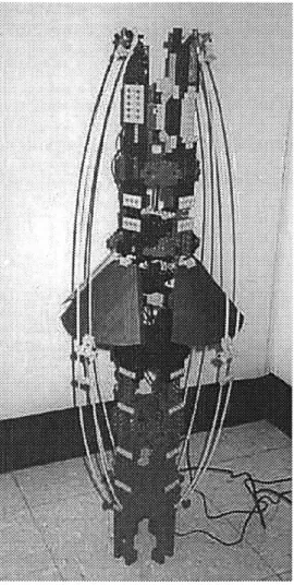
In order to achieve a closed and circular projected area, curved conical sections in the form of petals are attached to each external pivoting linkage bar. Hence, a variable pitch conical shape can be achieved provided each petal rides on its neighbor's side. A first design iteration was implemented using LEGO parts because of ease, low cost, and fast turn over. Figure 3.2 shows the outcome.

A total of four linkage arms are used in this bench level prototype. A LEGO MINDSTORMS

controller brick is used to control the linear actuator driving the linkage system. Flexible cardboard "petals" are mounted on each pivoting arm proving the idea of having a series of petals riding on each other's side to achieve a closed profile.

For purposes of experimentation we fixed a geometrical constraint on the prototype to be built. The tool's closed diameter should be no bigger than 2.5 inches since this is representative of most logging tools. The LEGO prototype gave a lot of insight into what should be incorporated in a more realistic prototype tool. First of all, the size constraint in the diameter of the tool restricts the number of linkage arms that can be used in order to achieve the umbrella mechanism. For the diameter chosen, the maximum number of linkage arms that can be packaged reasonably is six. Figure 3.3 portrays a final concept drawing of the umbrella tool, shown here without petals. The angle between each linkage arm is 60 degrees and each L-shaped pivoting bar is 1.5 inches long and 0.25 inches wide. In order to reduce the material and equipment requirements, we decide to test the prototype in a moderate environment using water at ambient temperature. Therefore, the final prototype was built using aluminum for the outer shell and stainless steel and brass for the linkage arms. All aluminum parts were anodized to achieve higher underwater durability. This greatly reduced the cost of manufacture since real downhole tools require specialized alloys, which are more expensive than the materials we used. Figure 3.4 displays the assembled linkage mechanism. Detailed machine drawings can be found in Appendix A.

Figure 3.4: Final Prototype linkage mechanism with petals attached.

3.2.2 Petals

The final problem to be addressed was to design petals flexible enough to accommodate the change in radius of curvature due to the opening and closing of the umbrella. When the umbrella is closed, the radius of curvature of each petal should be 1.25 in (tool radius), and at maximum opening the petals should bend to reach a radius of curvature close to the radius of the pipe where the tool is on. We decided to test the prototype in a 6 in I.D pipe, which fixed the requirements for the petals. Some alloys are flexible enough to be used as material for the petals but since petals ride on top of each other there might be problems with friction and abrasion if metallic parts are used. Therefore, we decided to use carbon fiber composites for the petals since they have comparable strength and in addition carbon fibers auto lubricate on sliding contacts.

The axial strengths of a composite matrix vary depending on the angle at which the matrix has been laid, the number of fiber layers used, and the resin used to bond the layers. The specifications for our petals were high radial stiffness and enough tangential stiffness to withstand differential pressure while still allowing the bending of petals without fracture. Different matrix angles and bonding compounds achieve fairly varied combinations of radial and tangential stiffness. We experimented using polyurethane and epoxy resins with different hardness along with several combinations of matrix layers and angles, and we

longitudinal axis of the petals. A medium hardness epoxy was used with only three layers of carbon fiber. In addition, a stainless steel insert was placed in the longitudinal axis of each petal to increase strength and minimize fracture problems due to the placement of mounting holes on the petals. The petals used in the prototype are displayed in figure 3.5. Each petal is 3.5

in

long and has a major circumference of 3.25

in

and a minor circumference of 1.3

in

.Appendix B contains the details of the composite petal fabrication.

Figure 3.5: Composite petals

3.2.3 Linear Actuator

Using the model developed in chapter 2 we estimated the pressure ranges that the umbrella mechanism would need to overcome while deploying inside a 6

in

I.D pipe with flows ranging from

0

to

10

(m

Is)

since these values are common in normal well operating conditions. It was determined that a maximum of

100

lb

is the force that the umbrella would need to overcome when closing. Under this restriction and the

imposed size

limitations

we choose a

linear

actuator from TS Products Inc [18]. The

linear

actuator is composed of a

1724

MicroMo brushless DC motor, a high-speed reduction gearbox, and a drivescrew. The maximum

load

that the actuator can overcome is 50

lb

while still in servo window, at a velocity of 25

mi/s / S

. The actuator will stall at 87

lb

.This clearly would not meet the requirements for high pressures

but would suffice to test the prototype in a fair range of downhole pressures. In addition, the actuator is only

1

inch in diameter and 7 inches

long,

and has a

1-inch

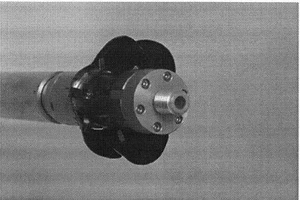
stroke, which perfectly fits inside our tool geometrical constraints. Figure 3.6 displays the linear actuator mounted on top of the umbrella mechanism.

Figure 3.6: Linear actuator attached to umbrella module.

The actuator needs to be protected against the environment, hence it was mounted inside a sealed housing and pressure seals were used at the connection with the umbrella mechanism. Drawings of the mounting parts and the sealed housing can be found in appendix A.

3.3 Position feedback module

Every logging tool has position sensors to monitor and record its position inside the well since this is crucial for correct interpretation of the logging measurements. The method most commonly used involves a casing collar locator (CCL) which, as it name stands for, is a sensor used to locate casing collars and other features of downhole hardware since these can be used as future depth references. There are two types that are available commercially: magnetic and mechanical CCLs.

Magnetic casing collar locators use a system of two permanent magnets, which produce characteristic magnetic fields. A deformation of either of the magnetic fields, produced by a gap between casing joints, or tubing hardware, is detected by a winding with high permeability core. The resulting electromagnetic imbalance is transmitted to the surface and depth correlated and can thus be recognized in the future as a downhole hardware arrangement [17]. Mechanical collar locators use feelers or finger mechanisms that produce signals that are sent to the surface whenever the feelers cross pipe connections or other downhole irregularities [17]. For the purpose of testing the obstruction module, the use of CCL technology would not be possible since it requires extra equipment. Therefore, a mechanical position feedback module was designed. Its operating principle is simple: A passive wheel is spring loaded against the tube wall so that as the module moves the wheel drives a zero-backlash belt. The belt connects to a high precision miter gear arrangement which drives a shaft connected, through pressure seals, to a an internal encoder. Figure 3.7 displays the module design, which was also built from aluminum with a special cavity to house an optical incremental encoder. Detailed machine drawings can be found in Appendix A.

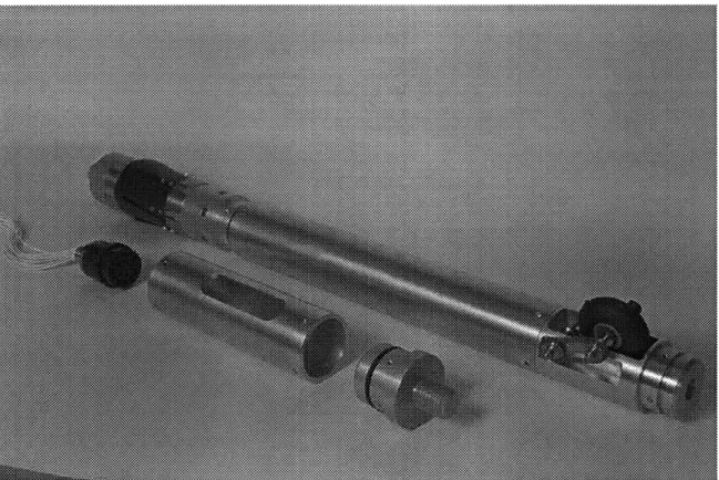
3.4 Complete Tool

The complete obstruction module is composed of the umbrella mechanism, the linear actuator housing and the position feedback module. These three sections are mounted between two centralizers when testing their dynamic behavior. The main goal of the project is to achieve an autonomous logging tool module that would perform adequately in a real well. However, for practical reasons the module was tested in a simulated well, and the hardware and software for the obstruction module were tested using a cable connection to the outside of a simulated well since these speed the debugging process. Figure 3.8 displays the three module parts in their normal arrangement, next to them are portrayed the special underwater cable connection for the tool and the section that houses the connection cable.

Figure 3.8: Complete Tool Arrangement.

The next step in our analysis is to identify experimentally the fluid losses brought by the obstruction shape chosen in our design.

Chapter 4: Loss Coefficient Identification

4.1 Experimental Setup

In order to identify experimentally the loss coefficient of the obstruction shape chosen we decided to perform static tests using a model of the obstruction tool. A simulated well section was designed and built in real scale in order to replicate downhole velocities and pressures. Multiphase flows are difficult to implement experimentally since extra hardware and controls are needed, and commercial pumps can handle mainly low viscosity liquids, therefore, the fluid media used for testing was single-phase water. The obstruction tool model was built at full scale with the same materials used for the real prototype in order to keep geometrical and physical proportions during the experiments. A description of the hardware used for the experiments and the criteria used for testing follows.

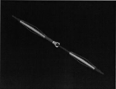
4.1.1 Tool Model

Prior to the fabrication of the umbrella prototype, a model of the real obstruction tool was built from solid aluminum in order to test its hydrodynamic properties. The model consisted of a shape similar to the umbrella mechanism mounted between two static centralizers as displayed in figure 4.1. Detailed machine drawings of the model can be found in Appendix A.

In order to test the umbrella shape, different aluminum cones were mounted and tested on the model. A total of four cones were tested, each one having a different combination of projected area and depth. Figure 4.2 displays two of the cones used for testing.

Figure 4.2: Aluminum Cones used to test the "umbrella" shape properties.

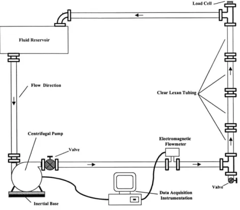
4.1.2 Flowloop

A diagram of the simulated well is portrayed in figure 4.3, the system is simply a flowloop composed

of a 20

ft

long straight section of clear cast acrylic tubing connected to a reservoir and a centrifugal pump. The pump is used to drain water from the reservoir plus circulate and control the fluid flow inside the clear tubing section. The entire structure is secured against a solid wall. Copper tubing is used to connect the pump inlet and outlet to the top and bottom of the straight section.

4--Fluid Reservoir

7

Flow Direction

Load Cell

-t

Clear Lexan Tubing

lye Centrifugal Pump Electromagnetic ValveFlowmeter Data Acquisition Inertial Base Instrumentation

Figure 4.3: Diagram of Flowloop Setup (not to scale).

4.1.3 Pump, Sensors and Hardware

The pump used in the flowloop is a centrifugal pump capable of delivering mass flow rates of 600

GPM

at 140

ft

of head (using water). The impeller is driven by a triphase, 30 Watt AC motor. The pump is mounted on an inertial base in order do damp any vibrations during operation. Figure 4.4 shows the pump and the inertial base.

A programmable controller regulates the pump operations. Consequently, accurate step, ramp and

sinusoidal flow inputs can be applied to the loop. For experimental purposes it is desired to measure accurately the flow rates inside the loop. Several choices of flow meters are available commercially. The most commonly used in industry are mechanical flowmeters or spinners and electromagnetic flowmeters. Spinners have one or several propeller blades that are put in contact with the flow, as the flow "spins" the blades they generate small voltages via dynamos. The voltages generated can be calibrated to the flow velocities and the output can be used to determine the flow rates. However, this kind of flow meter is not very accurate and disturbs the flow profile as well.

On the other hand, electromagnetic flow meters are very accurate and work under a principle that does not disturb the flow being measured. An electromagnetic flowmeter is essentially a piece of piping with an internal isolating lining. Two electromagnetic coils are located outside the flow tube, diametrically opposed to each other and protected by a carbon steel housing. Two electrodes, inserted into the flow tube, are positioned "flush" with the internal diameter of the tube and perpendicular to the coils. A pulsed DC voltage energizes the coils and a magnetic field is generated across the flow tube section. According to Faraday's law, when this magnetic field is "cut" by a conductive liquid flowing through the meter, a voltage is generated in the liquid. This voltage is directly proportional to the liquid flow velocity, and therefore to the actual volumetric flow rate of the liquid. Provided the liquids being tested have some conductivity the small voltages generated can be measured, and flow rates can be estimated with an accuracy of 0.25% or better.

An electromagnetic flowmeter was installed downstream from the pump outlet as shown in figure 4.5.

Care was taken to install the flowmeter more than 5 pipe diameters away from the pump outlet in order to have a fully developed flow for measurement. The tool model was submerged inside the long straight section of clear tubing and secured to a load cell mounted at the top T-junction in order to perform the static tests. The load cell mounting is shown in figure 4.6. The load cell used is a universal (tension/compression) hermetically sealed cell rated for 1000

lb.

This type of load cell, and in general any axial load cells, are very susceptible and can be very easily damaged by any bending or torsion applied. Therefore, special care was taken when mounting the model and a special feature was designed to take any bending moments applied to the cell while the setup was moved.

A reservoir is part of the flowloop to facilitate cleaning and replacement of the liquids. The reservoir

has a capacity of 800 gallons, is made of nylon, and is supported by four casters to ease its manipulation; figure 4.7 portrays how it was mounted to the flowloop.

Figure 4.7: Fluid Reservoir.

Finally, the readings (voltage outputs) from the electromagnetic flowmeter and the load cell are monitored using digital multimeters interfaced to a computer running LabView. A LabView program is used to filter the signals and convert them to the desired units for calculations. Figures 4.8 and 4.9 display the data acquisition equipment sitting next to the flowmeter and a front view of the entire flowloop.

Figure 4.9: Front view of Flowloop.

4.2 Experiments

As we explained briefly at the beginning of the chapter, the experiments performed were aimed to identify the loss coefficient brought by the umbrella mechanism. A tool model was submerged inside the straight section of clear plastic tubing and attached by a rigid connection to a universal load cell. The load cell was in turn rigidly mounted to the top T-junction so it would measure any force applied to the model inside the flowloop. Solid conical fixtures were used in the model in order to simulate the umbrella mechanism and a different conical geometry was tested in each experiment to simulate different umbrella openings and depths.

For a given experiment, with the model rigidly mounted inside the loop, a series of increasing flow rates step inputs are administered using the pump controller. The forces felt by the model and the flowmeter readings are continuously recorded using the data acquisition hardware. Once the components attributed to the weight and the buoyancy of the model are subtracted, the only force present is that due to the differential pressure across the obstruction. Figures 4.10 and 4.11 display the model being submerged

Figure 4.10: Model being submerged inside the flowloop.