Determining distributed source waveforms in casual, lossy, dispersive, plane-wave (CLDP) materials

Determining Distributed Source

Causal, Lossy, Dispersive, Plane-Wave

Waveforms in

(CLDP) Materials

R. Joseph Lyons

B.A. English, University Of Colorado (1986) M.S. Electrical Engineering, Boston University (1991)

Submitted to the Department of Electrical Engineering and Computer Science in Partial Fulfillment of the Requirements for the Degree of

Doctor of Philosophy in Electrical Engineering and Computer Science at the

Massachusetts Institute of Technology June 1998

@

Signature of Author

Certified by ...

Dep oEecric ngi wringand Computer Science Depar(A1t of Electrical Engi ring and Computer Science May 14, 1998

. ..

.... . .... ...

7

Pr jcip e-sech Engineer

Accepted by ...

Arthur C. Smith Chairman, Committee on Graduate Students Department of Electrical Engineering and Computer Science

MASSACHUSETTS INSTITUTE OF TECHNOLOGY

MAY 2

11999

Determining Distributed Source Waveforms in

Causal, Lossy, Dispersive, Plane-Wave (CLDP) Materials

R. Joseph Lyons

B.A. English, University Of Colorado (1986) M.S. Electrical Engineering, Boston University (1991)

Submitted to the Department of Electrical Engineering and Computer Science on May 14, 1998 in Partial Fulfillment of the Requirements for the Degree of

Doctor of Philosophy in Electrical Engineering and Computer Science

ABSTRACT

This thesis presents and employs novel mathematics for the inversion of linear, first-kind Fredholm integral equations (IEs) which have a time t dependent response signal, a space z dependent source waveform, and a kernel with time dependence (at each z) corresponding to the impulse response of a thickness z slab of causal, lossy, dispersive, homogeneous material through which planar disturbances propagate according to the wave equation. These materials are called CLDP materials; these IEs are called CLDP IEs. These novel mathematics are applicable to the PESAW (aka PEA) charge recovery method.

The proposed inversion method recognizes that the (temporal) Fourier transform of a CLDP IE's response signal can be interpreted as the values of the (spatial) Laplace transform of that IE's source waveform along a Laplace plane path determined by the material's propagation wavenumber k(f). Executing the Laplace transform inversion integral along this CLDP path yields an inverse CLDP IE which recovers the true source waveform provided that source waveform is real, causal, Fourier-transformable, and also satisfies the proposed k(f)-dependent 'CLDP criterion'. The forward and inverse CLDP IEs corresponding to a particular CLDP material model k(f) therefore comprise a particular integral transform relationship applicable to waveforms satisfy-ing the CLDP criterion for that material. The CLDP transform relationship for a

lossless/dispersionless material reduces to the (unilateral) Fourier transform.

Even without noise, the 'inverse CLDP'-recovered waveform gleaned from an abruptly bandlimited CLDP response signal requires regularization - a generalized Gibbs-Dirichlet kernel dubbed 'the Darrell' comes into effect. The measured (time sampled) PESAW signal is necessarily bandlimited; this thesis investigates regularization via lowpass filtering of the measured signal. Both synthetic and experimental examples are inves-tigated. The focus is on MHz-range signals culled from mm-range polymeric PESAW experiments. A method for determining the requisite model k(f) from measured PE-SAW signals is also presented and employed.

Thesis Supervisor: Chathan M. Cooke Title: Principal Research Engineer

Acknowledgements

* First of all I would like to thank my advisor, Dr. Chathan M. Cooke. You are the model for clear headed, practical scientific research. You asked the questions, questioned the answers, and kept me on the path. Truly, it would not have been possible nor nearly so memorable without you.

* I would also like to thank my mentors: Cooke (again), Hohlfeld, Horenstein, Mor-genthaler, and Zahn - for, well, mentoring.

* Thanks also to Marilyn Pierce, Kathy McCue, and Maxine Milstean - for believing in me and encouraging me to go on when going on seemed pointless. And for making the way more passable.

* And of course I would like to thank everyone else who acted like a friend to me during my grad school years. And so I will, starting with my family, roughly in order of appearance: Pop & T; Guille, Vicky, Erik; Moon, The Commandress, Gwynn, Carmen, Carol; Couga', Zane, Teresa, Gracie & li'l Zane; Joe, Jane, Stewart, Ben, Lex; Alfred, Johnnie Mike. And Rose, rose, rose ...

* Also Jessica, Rob & Gail Mills. Sarah Trickett. Kaarina & Jon. Mary Nell, Zachary Knight, and Rebecca Morss. Bart, Jamie, Terry, Eric, Anna, Jim, Jeff. Ollie. James Goodberlet. Siegfried Fleischer. Eric Mauer. John Barr. Bill Bresee. Jay Wasserman & Oribe. Also Hiroki Shigetsugu and Pam Ikegami. Yanqing Du, Alexander Mamishev & Kristina. And Priscilla and Caia & Amy and Ronnie. No way will I forget to thank

Judy Rudolph or Wayne Ryan. You know why. I thank Cecelia as well ...

* A big thanks to Sara Jamileh and Heather Heimarck, who were always there through thick and thin.

* Thanks to Melissa Collins, who saved me from going off the brink. More than once. * Thanks to Darrell "The Darrell" Schlicker, Greg Derderian & Rhonda - for listening to me talk about this thesis ad nauseam. Aaron McCabe and Mitch Meinhold did this too, and read and offered insightful comments upon early versions of the text. To Mr. Schlicker in particular: your comments and observations, and your finite width and asymmetry, were a boon and an inspiration, respectively.

* Thanks to the creators of the Macintosh, and also to the creators of Mathematica, LabVIEW, Igor, and Textures. You made my life easier.

* Last but far from least: consistent, steady support from the Tokyo Electric Power Company is acknowledged with deep gratitude. Especial thanks to Yoji (Naohisa Yoshifuji)!

Contents

1 Overview 10

1.1 Requisite Background Material ... ... 10

1.2 Thesis Motivation - PESAW & CLDP . ... 11

1.3 The Quasi-Static Approximation (QSA) ... 12

1.4 PESAW Essentials ... .. ... 12

1.5 The PESAW-CLDP Integral Equation ... 13

1.6 The Dominant Recovery ... ... 14

1.7 CLDP Materials, Paths, and Transforms ... 14

1.8 CLDP Inverse Transforms and the Darrell . ... 16

1.9 The Behavior of the Darrell ... ... 17

1.10 The Impact of the Darrell ... ... 18

1.11 The Need for Regularization ... ... 18

1.12 Possible Regularization Methods ... ... 19

1.13 Spatially Dependent BLG (SDB) Filtering . ... 21

1.14 The Lyons Recovery ... 22

1.15 Lyons Recovery vs Dominant Recovery . ... 22

1.15.1 skewness ... ... 24

1.15.2 w idth . . . . . . . .. . 24

1.15.3 position ... .... ... . 24

1.15.4 area . . . .. . 25

1.16 Preview of Experimental Results ... .... 26

1.17 Generality of the Lyons Recovery ... ... .. 27

1.18 Charge Recoveries: Motivation and Review . ... 28

1.18.1 Non-PESAW Methods ... 28

1.18.2 The PESAW Method ... ... 29

1.19 Thesis Outline ... . .... ... ... . 31

2 Technical Introduction 36 2.1 The PESAW Problem ... ... 36

2.2 From Voltage Signal To Charge Waveform . ... 40

2.2.1 Step 1 . . . .. . 41

2.2.2 Step 2 . . . . 41

2.3 Dimensions And Units . ... 2.3.1 Nepers and Decibels ... 2.4 The Need For Improved Recovery ... 2.5 CLDP Transforms ...

2.5.1 Group Velocity . ... 2.5.2 Time Domain Recovery. ... 2.5.3 The Convolution Inverse ... 2.5.4 The Group Signal ... 2.5.5 Conjugate Symmetry ...

2.5.6 Delay-Only Materials And The Fourier Transform . 2.5.7 Delay-Only Materials And The Dominant Recovery 2.6 The Darrell Property of the Inverse CLDP IE ...

2.6.1 The Darrell As Generalized Gibbs-Dirichlet Kernel 3 Loss, Dispersion, Deconvolution

3.1 Loss And Dispersion . . . .. 3.2 Deconvolution ... ... 4 The 4.1 4.2 4.3 4.4 4.5 4.6 4.7 4.8 PESAW Recovery

Bulk Forces And Plate Forces . ... Bulk And Plate Responses ... The Applied Voltage Signal Va(t) .. Resolving The Two Plate Responses Resolving The Bulk Response . ... Temporally Impulsive Electric Field . A Sample Pressure-Response Signal .

Calibration And Bulk Signals . ... 4.9 Sampling Issues .

4.10 Extracting The Experimental Impulse Response Si 4.11 Extracting The Attenuation Coefficient a(f) . . . 4.12 Extracting The Phase Velocity c(f) . . . . 4.12.1 A Possible Improvement . . . . 4.13 Curve Fitting And Parameter Extraction . . . . . 4.13.1 Frequency Domain Parameter Extraction . 4.13.2 Time Domain Parameter Extraction . . . 4.13.3 Final Note On Parameter Extraction . . . 4.14 Implementing The Lyons Recovery . . . . 4.14.1 Relationship To The PESAW Experiment

ignal He(t)

4.14.2 SDB Filtering (Items I & II)

4.14.3 Time Samples To Frequency Samples (Item III) 4.14.4 Frequency Domain Integration (Item IV) . . . . 4.15 Putting It All Together ...

4.15.1 Overview ... 56 56 58 62 62 . . . 64 . . . 66 . . . 67 . . . 67 . . . 68 . . . 68 . . . 69 . . . 71 . . . 72 . . . 72 . . . 73 . . . 75 . . . 75 . . . 75 . . . 76 . . . 77 . . . 77 . . . 78 . . . 79 . . . 80 . . . 82 .. . 83 .. . 83

111

4.15.2 The Need For Spatially Dependent Scaling ... 4.15.3 SD Filtering And The Spatial Sampling Interval ... 4.15.4 Determining The SDB Function fe(z) . ...

4.15.5 The Un-Normalization Procedure . ... 5 Inverting Linear, First-Kind Fredholm IEs

6 Causality And Materials

6.1 The Kramers-Kronig Relations ... 6.1.1 Example: Bromwich Materials ...

6.2 The Nearly-Local KK Relations . . . . 6.2.1 Example: Polymeric Materials . . . . 6.2.2 The Standard Model For Polyethylene . . . . . 6.3 The Paley-Wiener Criterion . . . . 6.3.1 Failure Of The Polymeric Model . . . . 6.3.2 Existence Theorem . ... . ... 6.4 The Paley-Wiener-Guillemin Criterion . . . .

6.4.1 Existence Theorem . . . . . . . .. 6.5 Analytic Propagation Coefficients . . . ...

6.5.1 Example: The Standard Skin-Effect Material. 7 CLDP Transforms

7.1 The Principal Insight ... ... .. 7.2 CLDP Paths ... .. ... ... 7.3 The Bromwich Path ... ... 7.4 The Bromwich Inversion . . . . . . . . .... 7.5 The Proposed Inverse CLDP IE ...

7.6 The Darrell Property of the Inverse CLDP IE . . . . . 7.7 Deriving the Darrell . . . . . . . . .. 7.8 Validation of the Inverse CLDP IE . . . . 7.9 The Darrell As Delta Convergent Sequence . . . .

7.9.1 The Basic Idea ...

7.9.2 Interpreting The Dirac Delta Function . . . . . 7.9.3 Darrell-Determined Constraints on Q(z) . . . . 7.10 Numeric Verification Of The Darrell Property . . . . . 8 The Lyons Recovery Applied To Synthetic Data

8.1 The Standard Impulsive Source Waveform . . . . 8.1.1 The Unregularized Recovery . . . . 8.2 The Standard Gaussian Source Waveform . . . . 8.3 The SIB Recovery ...

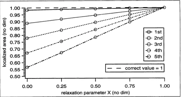
8.3.1 Relaxation To The Dominant Recovery . . . . . 8.4 The SDB Recovery ...

8.4.1 Plots Pertaining To The Relaxed SDB Recovery

94 . . . . . 95 . . . . . 96 . . . . . . . 97 .. . . . . 99 . . . . . 100 . . . . . 100 . . . 101 . . . . . . 101 . . . . . . 101 . . . . . 102 . . . . . . 102 . . . . . 103 106 . . . 106 . . . . . 108 . . . . . .. . 108 . . . . . 109 . . . . 110 . . . . . 111 . . . . . . . 112 . . . . . 113 . . . 121 ... 121 . . . 121 . . . . . 122 . . . . . 129 135 . . . . . 135 . . . . . 135 . . . 141 . . . . 143 . . . . . 146 . . . . . 151 . . . 151 90

9 The Lyons Recovery Applied To Experimental Data 164

9.1 The Voltage Boundary Condition ... 166

9.2 The Double-Sided E-beam Experiment ... 167

9.2.1 Inverse Medium Solution ... 167

9.2.2 Inverse Source Solution - Calibration Waveforms ... . 172

9.2.3 Raw Lyons-Recovered Localized Area . ... . 177

9.2.4 Un-Normalization And The Voltage BC . ... 186

9.2.5 Verifying the Voltage BC for Calibration Waveforms ... 186

9.2.6 Verifying the Voltage BC for Bulk Waveforms . ... 189

9.2.7 Closer Analysis Of The Bulk Signals . ... 192

9.2.8 Comparing Bulk Charge Recoveries . ... . 194

9.3 The Calibration Experiment . ... . .. ... .. 197

9.3.1 Inverse Medium Solution ... . . . . . . . . . 198

9.3.2 Inverse Source Solution ... .... ... . 201

9.3.3 Voltage Waveform Verification ... . . . . . 208

9.4 Overview Of The Remaining Two Experiments . ... 213

9.5 The DC Field Experiment . ... .. . . . . 213

9.5.1 Inverse Medium Solution . ... .. . 213

9.5.2 Inverse Source Solution - Calibration Waveform . ... 217

9.5.3 Inverse Source Solution - Bulk Waveform . ... 219

9.6 The Distal Dipole Experiment . ... . . 222

9.6.1 Inverse Medium Solution . ... . . . . 222

9.6.2 Inverse Source Solution - Calibration Waveform . ... 225

9.6.3 Inverse Source Solution - Bulk Waveform . ... 227

10 Conclusions And Surmises 236 10.1 Conclusions ... . .. . . .... .. .. ... . . . . . . . .. 236

10.1.1 CLDP IEs ... . ... . 236

10.1.2 Inverting CLDP IEs ... 237

10.1.3 Group Velocity ... ... ... 239

10.1.4 CLDP Theory And The PESAW Charge Recovery ... 240

10.1.5 The Darrell ... ... 241

10.1.6 Synthetic Validation Of The Lyons Recovery . ... 242

10.1.7 Experimental Validation Of The Lyons Recovery ... 243

10.1.8 Overall ... ... 244

10.2 Surmises . ... .. ... . . 245

10.2.1 Recovery From Inhomogeneous Materials . ... 245

I Appendices I

A Wave Equation Transfer Function 248

B The BLG Filter B(fe, f) And The Standard SDB Function fc(z) 252

B.1 The Filter B(f,, f) (Blackman's Lucky Guess) ... 252

B.2 The Standard SDB Function fc(z) ... 253

C Data Describing The Three Standard Materials 255 D Graphical Depiction Of The Principal Insight 259 E Key Concepts & Notation 262 E.1 Bars, Tildes, Hats, Checks ... 262

E.2 Acronym s ... ... 264

E.3 Signals, Waveforms, Standards ... 264

E.4 Functions Describing Experiment & Recovery ... 265

E.5 The Meanings OfK: ... ... 265

E.6 The Derivative Of IC(f) ... ... 266

E.7 Lyons Recovery vs Inverse CLDP IE ... 266

E.8 CLDP Transfer Function ... 266

E.9 The Darrell ... ... ... 267

E.9.1 fm vs fmM ... 268

E.10 Subscripts: Usual Meaning, Example ... 269

F Transform Definitions 270 F.1 The Fourier Transform ... ... ... 271

F.2 The Laplace Transform ... ... . . 271

F.3 The Fast Fourier Transform . ... ... 272

F.4 The Hilbert Transform ... .. ... 272

F.5 The CLDP Transforms ... ... 273

G PESAW-CLDP Overview 274

List of Figures 275

List of Tables 282

Chapter 1

Overview

1.1

Requisite Background Material

information in this short

thesis easier to digest if he first familiarizes himself with the section and appendices E, F, and G.

+ Va(t) + pulse + + Transducer + V(t) .4 -P(t) + HT(t) + + proximal + distal capacitor + capacitor plate q, plate

I

I

I

z

1

Figure 1.1: The PESAW data collection apparatus: a parallel-plate capacitor with a pressure-to-voltage transducer HT(t) attached to its proximal plate. Also shown: a column of plusses representing a hypothetical embedded surface charge layer ql at position z = zl. Not shown: surface charges generated on the inside surface of each plate in response to both the bulk charge Q(z) = q16(z - zl) and the applied voltage

Figure 1.1's charge waveform Q(z) = q,6(z - zl), where 6(z) is the Dirac delta function and ql is measured in units of nC/cm2. The position z (distance from the

proximal plate) is measured in millimeters, so Q(z) has units nC/(cm2 mm). The applied, pulsive excitation voltage Va(t) is the impetus for the measured voltage V(t). The Coulomb force F(z, t) = Q(z) Va(t) / provides the coupling between them.

Note that there will also be surface charge on the capacitor plates. Some of this plate charge is constant over the acquisition time of the PESAW signal - the image charges corresponding to the embedded charge waveform Q(z). Some of this capaci-tor plate charge is time varying - the surface charge C' Va(t) due to the time varying voltage Va(t) applied to the capacitor C' = e/1, where e is the permittivity of the

capac-itor's dielectric and 1 is the distance between the plates. Bear in mind that the desired, experimental Q(z) will generally be a continuous function of position z. Figure 1.1's spatially impulsive Q(z) is introduced for didactic purposes only, to simplify the anal-ysis.

1.2

Thesis Motivation

-

PESAW & CLDP

The motivation for the research that led to this thesis was the desire to improve the Pulsed Electrically Stimulated Acoustic Wave (PESAW, aka PEA; see section 1.18.2) charge recovery method. Figure 1.1 depicts the PESAW data collection apparatus. The applied excitation voltage pulse Va(t) is the impetus for the measured voltage V(t). The Coulomb-force interaction F = Q E between the embedded charge waveform Q(z) and the Va(t)-generated excitation electric field E(z, t) provides the coupling between Va(t) and V(t).

In this thesis' one-dimensional planar geometry E(z, t) = Va(t)/l is independent of z. However, other geometries (eg: coaxial cable) yield E(z, t)'s that are not independent of z. In the interests of generality, this thesis' results are presented in terms of the general E(z, t) instead of this thesis' particular form E(z, t) = Va(t)/l.

Over the duration of the excitation pulse the excitation electric field generally causes bulk charges to move slightly from their pre-excitation positions, in accordance with Hooke's law F = - K X [83]. The electric field does (spatially distributed) work on the dielectric, which stores the energy in the form of distributed compression.

Just after the excitation pulse has been applied (time t = 0+) the distributed compression starts to uncoil into kinetic energy, launching a compressional wave toward the proximal capacitor plate (and also toward the distal plate, although with opposite polarity. This thesis focusses upon the wave launched toward the proximal plate.).

In the PESAW context, CLDP theory applies to the mapping between this initial, distributed source (pressure) waveform and the response (pressure) signal P(t) it would cause to pass through z = 0 if the dielectric region continued for negative z.

1.3

The Quasi-Static Approximation (QSA)

If the duration of the pulsive Va(t) is much longer than the time required for an electromagnetic wave to traverse the capacitor then, according to the quasistatic ap-proximation (QSA,[86]), Va(t) will generate a temporally pulsive, spatially distributed E(z, t) proportional to the product of the signal (function of time alone) Va(t) and some waveform (function of space alone) E~ (z) that depends only upon the capacitor's geometry (see section 2.2.3).

Under the QSA the force F(z, t) = Q(z) E(z, t) oc [Q(z)Ez(z)]Va(t) must also have separable space and time dependencies, and the time dependence of F(z, t) must also be given by Va(t). Therefore the actual signal V(t) measured as a response to a finite duration Va(t) will be simply related to the hypothetical signal Vb(t) that would be recorded if the time dependence of F(z, t) were truly impulsive: V(t) Oc V (t) * Va(t), where the * denotes convolution.

So although it is physically impossible (see section 4.6) to have a temporally impul-sive F(z, t), under the QSA it is as reasonable as it is simplifying to think of F(z, t) as having the separable, temporally impulsive form F(z, t) = Q(z)&(t) where 6(t) is the Dirac delta function.

The proceeding discussion speaks of applying an impulsive excitation voltage Va(t) =

V6(t) to generate spatially distributed, temporally impulsive fields E(z, t) and F(z, t).

According to the above discussion, this approach to analysis of the PESAW experiment makes sense provided the QSA holds. Throughout this thesis, it will be assumed that the QSA holds.

The following chapter's more rigorous analysis introduces a meaningful Q(z) = VQ(z)/l which has units of pressure (Pascals, Pa) per velocity (millimeters per mi-crosecond, mm/[s). Therefore, dividing Q(z) by [Pa ps] yields a normalized Q(z) with units mm-'. Similarly, dividing P(t) by [Pa ps] yields a normalized P(t) with units ps- 1. The same notation (Q(z) and P(t)) is used for both the normalized and the un-normalized (physical) quantities. It is in this manner that the physical, PESAW quantities are generalized into the larger CLDP context.

1.4

PESAW Essentials

With P(z, t) representing a -z directed, Coulomb-force-generated pressure wave travel-ling through the dielectric after the pulsive Va(t) = V6(t) has been applied, the PESAW method seeks knowledge of P(t) = P(O, t), and the frequency dependent attenuation coefficient ca(f) and phase velocity c(f) of pressure waves inside the dielectric, as a means to determine first Q(z) (oc P(z, 0+)), and then (using Ez(z)) the desired charge versus position waveform Q(z).

Expanding on the preceeding discussion, this thesis' essential PESAW concepts are -1. that a -z directed travelling pressure wave P(z, t) will be launched by the

spa-tially distributed PESAW excitation electric field E(z, t) with the assumed-one-dimensional, spatially distributed charge waveform Q(z) inside the dielectric. 2. that the temporally pulsive pressure signal F(zo, t) oc Q(zo)Va(t) injected into

the dielectric by the charge layer at position zo will be modified (via a(f) and c(f)) as a result of having propagated through the slab of dielectric between that charge layer and the proximal capacitor plate

3. that the modifications imposed upon each layer's injected pressure signal will depend upon that layer's position because the thickness of the intermediate slab depends upon that layer's position

4. that this travelling pressure wave will, after having been modified, eventually impinge upon the proximal capacitor plate

5. that some of this impingent pressure wave will be transmitted through the ca-pacitor plate and into the transducer, where it is ultimately registered as V(t) =

HT(t) * P(t)

6. that the measured V(t) therefore contains 'tangled' information about the desired source charge waveform Q(z)

7. that information about Va(t), HT(t), a(f), and c(f) is required to 'un-tangle' the information in the measured V(t) and arrive at some estimate to the source pressure waveform Q(z) - R(z) which can then be mapped, via Ez (z), to an estimate for the desired charge waveform Q(z)

As a practical matter, the transducer depicted in figure 1.1 is often comprised of a delay line with a piezoelectric device attached to its left hand side. Some of the pressure waves P(z, t) travelling through the dielectric are transmitted through the proximal plate and into the delay line. These pressure waves eventually arrive at the piezo device and cause it to emit a voltage signal which can be sampled and stored by a digitizing oscilloscope. The delay line is added so that the electrical transients generated by Va(t) will have mostly decayed away by the time the desired, slower-travelling, pressure-wave signal is recorded by the oscilloscope.

1.5

The PESAW-CLDP Integral Equation

Chapter 2 of this thesis derives a linear, first-kind Fredholm integral equation (IE) model of the forward problem which expresses the response signal P(t) as the integral over position z of the product of the source waveform Q(z) with a position-dependent impulse response function H(z, t) that takes into account the propagation properties of the dielectric. That is,

P(t) =

j

Experimental factors such as the sample thickness I and the applied voltage have been normalized out so that Q(z) has dimensions of inverse length, and p(t) and H(z, t) have dimensions of inverse time. This normalization procedure is discussed in more detail in sections 2.2 and 2.3. A one-page overview of the CLDP-PESAW connection may be found in appendix G.

1.6

The Dominant Recovery

Setting aside, for now, a discussion of this normalization procedure and the methods used for reducing the influence of systematic errors and noise upon the measured sig-nal, the dominant method for mapping temporal signals to spatial waveforms simply maps time to space via some constant velocity Cd. This dominant recovery Rd(Z) corre-sponds to the assumption that acoustic waves inside the dielectric propagate without attenuation or dispersion (see sections 2.5.6 and 2.5.7). The result

1

1

r"

Rd(z) = -p(-) = - .(f) exp(j 27rflc(f)) df (1.2) Cd Cd Cd -oo

yields a perfect recovery provided that pressure waves passing through the material are only delayed, not attenuated or dispersed, so that

H(z,t) = 6(t - -) Hd(z,t)

Cd

where 6(t) is the Dirac delta function. Such a material is called a delay-only material.. When it was found that pressure signals measured by the PESAW apparatus could be interpreted to yield frequency f dependent estimates for the attenuation coefficient a(f) and phase velocity c(f) of pressure waves travelling inside the dielectric (see sections 4.11 and 4.12), the following question naturally arose: how can this information be used to improve the time to space mapping algorithm?

1.7

CLDP Materials, Paths, and Transforms

The previous section ended by asking how information about a(f) and c(f) could be used to improve the time to space mapping algorithm. This thesis' answer to that question was found to be, in some sense, larger than the question that prompted it. The result is that, if the dielectric is a CLDP material (Causal, Lossy, Dispersive, Plane-wave; see the abstract, or chapter 2) then there exists an inverse CLDP IE that exactly undoes the forward CLDP IE. The CLDP forward and inverse problem IEs

comprise an integral transform relation which relate spatial waveforms to temporal signals, and vice-versa. These transform relations are unilateral in the sense that all the spatial waveforms and the temporal signals treated must be causal, meaning each must vanish for negative values of its respective argument (z or t).

Bear in mind that, owing to the uniqueness of the Fourier transform, the information in each temporal signal could equally well be represented in the frequency domain. That is, the time domain signal P(t) possesses the same information as the frequency domain signal given by its Fourier transform

2(f).

Although PESAW data is collected in time, and although these CLDP transform relations could be expressed as space-time transformations, the mathematical analysis and computer implementation are simpler if the CLDP transform relations are thought of as space-frequency transformations. From the CLDP transform point of view, func-tions of space alone (waveforms) are considered to be direct-space funcfunc-tions whereas functions of frequency alone or time alone (signals) are considered to be inverse-space

functions.

Because each CLPD material corresponds to a unique integral transform relation, and because there are an infinite number of CLDP materials, this result amounts to the discovery of an infinite number of transform relations. This set of transform relations are called the CLDP transforms.

For example, the familiar Fourier transform relation is that member of the set of CLDP transform relations which corresponds to the delay-only material characterized by Hd(Z, t). That is: letting I -- oo, inserting the delay-only H(z, t) into the forward IE expression for P(t), and then Fourier transforming both sides of the IE yields a scaled, unilateral version of the Fourier transform. The dominant recovery Rd(z) yields a scaled version of the inverse Fourier transform. See sections 2.5.6 and 2.5.7.

This thesis' demonstration of the correspondence between a CLDP material and its associated transform relation utilizes the realization that the Fourier transform

2(f)

&(f) = a(f) +j 27rf/c(f) -Z(f)

where the familiar temporal Laplace transform variable s has been replaced by the spatial Laplace transform variable C so that

5 = o + jW

S= a + jp

This correspondence between P(f) and the spatial Laplace transform Q(&) of Q(z)

is detailed in chapter 7. The result is that, if

Q(IC)

= Q( (f) + j 3(f) )

= Q( a(f) +j 27rf/c(f) )

For now, suffice to say that if the Fourier transform Q() of the source pressure wave-form Q(z) exists, application of the Cauchy-Goursat theorem to the analytic [56, 57] Laplace plane region between the j 3 axis and the CLDP path results in the realiza-tion that the CLDP transforms merely exploit the independence of path of Laplace transforms.

1.8

CLDP Inverse Transforms and the Darrell

The added import of CLDP materials, paths, and transforms follow from the requisite exponential form of the Fourier transform H(z, f) of a CLDP material's temporally causal impulse response function H(z, t). For these materials, the source waveform recovery R(fm, z) given by inserting an abruptly bandlimited response signal P(fm, f) into the inverse IE can be shown to be the convolution of the true source waveform Q(z) with a waveform called the Darrell D(fm, z) which is determined solely by the CLDP material's properties a(f) and c(f) (or simply

K(f)),

R(fm, z) = Q(z) * D(fm, z)

where the * denotes spatial convolution and "the Darrell" D(fm, z) is given by

D(fm, Z) = m{ exp(z

C(fm)))

7rZ

= exp(z

a(f))

7rz

Note that the Darrell can be rewritten in terms of the two functions A and A of fm:

D(fm, z) = exp(z/A) sin(27rz/A)

7rz

where

-

c(f

)

f

1

A = A(fm)

-The function A(fm) does not depend on the material's attenuation coefficient a(f); the function A(fm) does not depend on the material's phase velocity c(f). And yet A and A are not truly independent; the functions a(f) and c(f) are linked because they must correspond to a causal material.

Raising the bandlimiting frequency to infinity results in the exact inverse transform. Therefore the fm - oo limit of any CLDP material's Darrell must converge to the Dirac delta function. That is, the Darrell is a delta convergent sequence in fm provided a(f) and c(f) describe a causal material.

The form of D(fm, z) ensures this convergence provided that the quantities [a(f)] and [f/c(f)] exhibit appropriate asymptotic behavior in the limit f -+ co. (see the

Technical Introduction's section titled The Darrell As Delta Convergent Sequence). If some test function varies slowly over every region of width A < A then D(fm, z) acts like a delta function for that test function, at least for z < A.

This result is consistent with the interpretation of the Darrell as a generalized Gibbs-Dirichlet kernel: just as the usual Gibbs-Dirichlet kernel (a sinc function [53, 77]) converges to a Dirac delta function as the bandlimiting frequency approaches infinity, so too does the Darrell. (see the Technical Introduction's section titled The Darrell As Generalized Gibbs-Dirichlet Kernel).

But real PESAW data is sampled at a finite time step At which corresponds to a finite fm = (2At)- 1 for which, generally, a(fm) > 0. Therefore an analysis of the

finite fm 'lossy Darrell' is of critical import if these CLDP transforms are to be used

to perform actual numeric recoveries. A numeric CLDP IE source waveform recovery which uses analytic CLDP transform mathematics is called a Lyons recovery.

1.9

The Behavior of the Darrell

This thesis' analyses assume 0 < A< A < oc, in which case the Darrell has * a central pulse - centered asymmetrically about z = 0

- with full width at first zero crossing (FWZC) = c(fm)/fm = A - with height HD - lim{z - 0} [D(fm, z)] = 2fm/c(fm) = 2/A - with area A = lim

{(

- with full width at half maximum (FWHM) ! A/1.66 * sidelobes that - oscillate with wavelength A

- grow without bound for z > A

1.10

The Impact of the Darrell

Applying the Darrell property to a material with Nq spatially impulsive embedded sources (excited by an electric field of short duration)

Nq

Q(z) = qn 6(Z - Zn)

n=l

yields the prediction that the recovery gleaned from noiseless PESAW pressure data sampled and processed 'without numeric error' at a finite time step At (and therefore finite f, = fM -- (2At)-1) will be given by

Nq

R(fm, z)= D(fm, -- z)

n=1

in the limit as At -+ 0 and (Nt At) -* oc, where Nt is the number of time samples.

1.11

The Need for Regularization

Applying this direct version of the Lyons recovery to real PESAW data acquired when

a(f,) does not vanish will result in a source waveform recovery that is desperately in

need of regularization.

That is, even if Q(z) consists of only a single source impulse the recovered waveform will exhibit significant yet unphysical oscillations, especially for positions A deep or deeper than that source impulse (see section 8.1.1). The reason is that the exp(a(fm)z)/z factor in D(fm, z) grows without bound for large z. When multiplied by D(fm, z)'s os-cillatory sin(27rfmz/c(fm))/wr factor, the result is a waveform that oscillates and grows without bound for large z.

Even if Q(z) is comprised of only two source impulses separated by a width W - A,

the recovery of the deeper source may well be completely obfuscated by the oscillations associated with the recovery of the shallower source. Even if A < W << A, the A oscillations associated with the recovery of the shallower source will be detrimental to the recovery of the deeper source. It follows that the recovery of a continuous charge distribution will be troubled as well, especially if its width W > A.

1.12

Possible Regularization Methods

Because only a material model and a sampling rate are required to compute some material's Darrell, and because the Darrell property involves only convolution of the true source waveform with the Darrell, one possible solution to this problem would seem to be simple deconvolution. Unfortunately, the Darrell has no Fourier transform (because of its exp(z c(fm)) term). Seen another way, deconvolution is impossible to implement because the Darrell, and consequently the entire recovery, are unbounded and impossible to parse.

Further, any parsed approximation to the Darrell would tend to be sinc-like. Be-cause the Fourier transform of a spatial sinc function vanishes for wavenumbers (inverse lengths) greater than some cutoff wavenumber, the usual Fourier domain deconvolution technique of division in the wavenumber domain is ill-posed. This is but a particular instance of the general rule that deconvolution tends to increase noise. The decon-volution problem is discussed in greater detail in the chapter titled Loss, Dispersion, Deconvolution.

A second possibility is to use the fact that the usual frequency domain inverse CLDP IE (2.31) can be expressed in the time domain (2.40) as a linear IE with the measured P(t) as the source, and the fact that causality requires that the plate pressure response to deeper charges arrive later than the response to shallower charges, to legit-imize performing separate recoveries for temporally localized 'chunks' of the measured pressure signal, then ensuring that the recovered waveform associated with each chunk does not extend significantly deeper than it ought. A third possibility advocates spatial filtering of the recovered waveform to explicitly suppress the troublesome characteristic wavelength A.

Many useful linear, spatially independent spatial filters can be described via convo-lution with a unit-area waveform which has its center of area at the origin. The 'boxcar waveform' with height A- 1 in the range -A/2 < z < A/2, and zero height elsewhere, is the member of this class of waveforms which takes most obvious advantage of the fact that the sidelobes go through one complete cycle in one A range, whereas the central pulse has all positive area in the same range.

The result D.(fm, z) of convolving D(fm, z) with this boxcar waveform is

DA(fm, z) = [ID(f, + A/2)- ID(fm, Z- A/2) - [U(z + A/2) - U(z - A/2)]

where U(z) is the Heaviside unit step function and the integral ID (fm_, z) of D(fm, z) is expressed in terms of the exponential integral Ei(Z) [52]:

I(fm, z) - D(f,, z') dz'

i= E(z[a(fn)+j 2irfm/c(fm )]) - i(z[a(fm) -

j

The result I, (f,, z) follows directly from the definition of Ei(Z) once the sin term in D(fm, z) is expanded in terms of complex exponentials via Euler's identity. The unit step component of DA(fm, z) arises from the fact that the exponential integral Ei(Z) is not analytic at Z = 0. Ei(Z) has a branch cut along the negative real axis of Z.

The impact of the branch cut is that when computing the definite integral of D(fm, z), the result gleaned via ID (fm, z) and the fundamental theorem of calculus is unity greater than the result gleaned via numerical integration of D(fm, z) if the integration range includes z = 0. Plots of D (fm, z) show that it exhibits a significant reduction in sidelobe envelope when compared with the unregularized D(fm, z). Like D(fm, z), D.(fm, z) oscillates and grows without bound for z > A.

In addition to standard (linear) wavenumber domain spatial filtering, the nonlinear median filter may also be useful. The median filter operates upon samples in the space domain by replacing the sample at position z, with the median value of all the samples within some neighborhood zo,±L,/ 2. The result is a filter that tends to remove large (greater than 1/L,) wavenumber variations from the waveform, while preserving edges. The median filter preserves slope. If Ln A, the procedure of integrating the direct recovery, applying the median filter, then differentiating tends to remove the A oscillations while preserving the central pulse.

It is also possible to decrease the sidelobe envelope of the recovery R(fm, z) by averaging the results of a number of recoveries utilizing various values of fm (denoted fi to distinguish them from the constant fm) where all the f 's are less than or equal to fm. The basic idea is that the central pulses will tend to add whereas (hopefully) the oscillating sidelobes will tend to cancel. Consider averaging the result of two Darrells: one with f', = fm and one with fm = fm/2. The result

D(fm, Z) + D(f/2, z) fm 3

D2 (fm, ) z) = cos(2r-z/c(fm)) D(- fm, z)

2 4 4

corresponds to an effective Darrell whose sidelobes decrease (via the slowly varying cos term) in the vicinity of its central pulse, which is about 33% wider than D(fm, z)'s central pulse. However, because the cos term is a continuous periodic waveform with range (-1,1), the sidelobes still oscillate everywhere and grow without bound for z > A. The characteristics of the recovery given by averaging all the f" 's between fm/2

and f_m is determined by the effective Darrell

_m1 ) c(fm) sin(ir fz/c(fm)) 3

which has a central pulse width that is still only about 33% wider than D(fm, z)'s central pulse, but which has a sidelobe envelope that is smaller than D(fm, z)'s by a factor of at least order z over all space. Like D2(fm, z), Do(fm, z)'s sidelobes oscillate everywhere and grow without bound for z > A. But perhaps the slower growth rate of the sidelobe envelope could be used in conjunction with one of the other possible regularization methods to yield an acceptable overall recovery.

1.13

Spatially Dependent BLG (SDB) Filtering

2(f) -+

k(fc,

This technique has been found to regularize the noiseless Lyons recovery and it removes high frequencies which often have, at least in the practical PESAW context, a low signal to noise ratio. Its result is called the SIB recovery (Spatially Indepen-dent Blackman) and should not be confused with the spatially filtered recovery which operates upon the recovered waveform.

This SIB recovery, although satisfactory in terms of regularization alone, has demon-strated the less-than-optimum property that the full width at half maximum of recov-ered source impulses are roughly independent of source position - intuition suggests that the FWHM of shallow-source recoveries ought to be smaller than that of deep-source recoveries. This intuition follows from the realization that pressure waves gen-erated by deep sources have to travel through more attenuative, dispersive material than do the pressure waves generated by shallow sources.

Theoretically, in the absence of noise, these deeper sources should be equally as 'recoverable' as shallow sources. But practically, the finite noise level in the mea-sured signal renders the more-attenuated signals generated by arbitrarily deep sources indistinguishable from the measurement noise.

It is possible to implement a modification of the SIB recovery in which the cutoff frequency f, of the BLG filter B(fe, f) used on P(f) is a function of z:

(f (z, f) P (f) B(f (z), f) (1.3)

This technique is called spatially dependent BLG (SDB) filtering. The quantity fe(z) is called the SDB function; see sections 4.14.2 and 4.15.4, or appendix B.

It has been found that the SDB filtered recovery can be made to yield a regularized recovery for which the FWHM of shallow-source recoveries is smaller than that of deep-source recoveries.

There is no inherent tie between the concept of spatially dependent filtering and the BLG filter. Future research may even show that the BLG filter should not be used for Lyons recoveries because its extreme rejection of frequencies above fc may not be necessary, and may tend to decrease resolution.

Nevertheless, SDB filtering is the only regularization method investigated in this thesis. The SDB filtering method was chosen as the workhorse regularization scheme in this thesis because the BLG filter has an historic association with the PESAW method, it is simple to implement, and it gives reasonable results.

1.14

The Lyons Recovery

A Lyons recovery is defined as the process, or the result, of numerically implementing the analytic CLDP inverse transform relation (2.31) defined by some material's prop-agation coefficient K(f). There are, therefore, many possible implementations of the Lyons recovery. But unless noted otherwise, in this thesis 'the Lyons recovery' refers to the SDB filtered Lyons recovery given by (4.60).

As defined above, the Lyons recovery does not pertain particularly to the PESAW recovery of the charge waveform Q(z) from the measured waveform V(t). Rather, the Lyons recovery pertains to the CLDP inverse source problem of mapping the generic frequency-domain response signal

k(f)

With this definition, the Lyons recovery is applicable to problems beyond the PE-SAW context. It is possible to validate the best-case efficacy of the Lyons recovery by synthetically generating a (to within numerical errors) noiseless P(t) via the stan-dard model (see section 6.2.2) for the propagation coefficient Kp(f) of polyethylene, and then performing a Lyons recovery upon the fast Fourier transform 1(f) of the synthetic, sampled P(t). The following section compares the Q(z)'s gleaned from this best case P(t) by the dominant recovery, and by the SDB filtered Lyons recovery.

As defined in (1.2), the dominant recovery Rd(z) does not use P,(f) whereas the Lyons recovery does. Similarly, Rd(z) does not use filtering whereas the Lyons recovery does. The approximately noiseless property of the data therefore gives the dominant recovery an unrealistic advantage for z 0 where the effects of attenuation and dis-persion have not had much distance over which to accumulate. Over larger distances, however, the Lyons recovery's use of

K,(f)

(in exchange for regularization) imposed by its use of SBD filtering.

1.15

Lyons Recovery vs Dominant Recovery

The following figure offers a comparison of the best-case SD filtered Lyons recovery R(z) to the best-case dominant recovery Rd(Z) for a source waveform comprised of ten impulses placed at half-millimeter increments, from z = 0.25 mm to z = 4.75

mm, inside a slab of what this thesis has dubbed 'standard polyethylene' (see section 6.2.2). The so-called standard model of polyethylene ultimately amounts to a specific {a(f), c(f)} pair. The specific {a(f), c(f)} pair selected for the model called 'standard polyethylene' was chosen because its values are typical for polyethylene.

This standard model of polyethylene (PE) will be widely used throughout this thesis. It will be introduced in the chapter titled Causality And Materials. This placement of sources is dubbed the standard impulsive source waveform. In this section, each of the sources is a spatial impulse, or Dirac delta function 6(z). The Dirac delta function is the limit of a (normalized) Gaussian as the Gaussian's width vanishes. Later in this thesis, this standard source waveform will employ Gaussians of nonvanishing width. 40 E 35 E 30 - R(z) r 25 ... Rd(Z) a 20 o 15 10 5 0.0 0.5 1.0 1.5 2.0 2.5 3.0 3.5 4.0 4.5 5.0 position z (mm)

Figure 1.2: Comparison of the noiseless Lyons recovery R(z) to the noiseless dominant recovery Rd(Z) for the standard source waveform embedded within standard polyethy-lene.

Note that the SDB filtered Lyons recovery has been denoted R(z), not R(fm, z). The

fm in R(fm, z) has been dropped for two reasons. First, because Blackman filtering

k(f)

Henceforth R(fm, z) will denote the Lyons recovery obtained from a

R(f)

appendix B. Note that SDB filtering reduces to spatially independent filtering if fe(z) is a constant fc, and that SDB filtering reduces to no filtering if f' = oo00.

The material model and source placement used here is consistent with this thesis' goal of establishing the efficacy of the Lyons recovery to PESAW charge recoveries of up-to-five mm samples of PE. Explicit presentation of P(t) has been omitted here because the Rd(z) presented in Figure 1.2 is simply a version of P(t) which has been scaled by the velocity Cd = 2.035 mm/ps. A plot of this P(t) can be found on page 45 in Figure 2.2.

1.15.1

skewness

Returning to Figure 1.2, note that the Lyons recovery is clearly better than the dom-inant recovery in terms of both the skewness of the recovered source impulses and in terms of their width. As for skewness, the recovered sources determined by the Lyons recovery are all nearly symmetric and have, therefore, nearly vanishing skewness whereas the recovered sources determined by the dominant recovery all have significant positive skewness (they all have long 'tails' extending to the right).

1.15.2

width

As for the width of the recovered source impulses, note that the z > 2.5 mm source impulses recovered by the dominant method fail to have a region between them in which the recovery vanishes, whereas all the source impulses recovered by the Lyons method do have a nearly-vanishing recovery region separating them. More quantitatively, figure 1.3 depicts a comparison of the position dependent FWHM of the source impulses recovered via the Lyons method (FWHM,(z)) to the FWHM of the sources recovered via the dominant method (FWHMd(z)).

Note that FWHM,(z) < FWHMd(z) for all z > .75 mm. The small width of the z < .75 mm source impulses recovered by the dominant method is due to the fact that no filtering was utilized to produce Rd (Z)

The small width of these recovered source impulses is an artifact of the known noiselessness of the data - when operating upon real (noisy) data the dominant recov-ery would presumably employ filtering, which would surely and significantly increase especially the small-z FWHMd(Z). It is encouraging that the Lyons recovery, which employs a significant degree of filtering, fares as well as it does when compared to the unfiltered Rd(z).

1.15.3

position

Closer inspection of the data depicted in figure 1.2 shows that the Lyons recovery betters the dominant recovery in terms of positional accuracy as well. The value Cd = 2.035 mm/ps was chosen to ensure that the dominant recovery's placement of the peak of the 4.75 mm source was exact. Given this constraint, the root-mean-square

280 - - FWHMd -240 _--- FWHM₁ ,. . E 200 ,e 2 160 136.32 lm , 95.49 m 120 LL 80 40 0.00 0.50 1.00 1.50 2.00 2.50 3.00 3.50 4.00 4.50 5.00 position z (mm)

Figure 1.3: Comparison of the position dependent FWHM of the sources recovered via the Lyons method to the FWHM of the sources recovered via the dominant method for the standard impulsive source waveform embedded within a material described by the standard model of PE

error (RMS) in the dominant recovery's placement of the ten source impulses is 16 pm, whereas the Lyons recovery's RMS placement error was just 1 pm.

1.15.4

area

The Lyons recovery bettered the dominant recovery in terms of the raw area of the recovered sources as well. Integrating between -0.25 and 5.25 mm, each raw recovered area fell short of the expected area of ten; the Lyons recovery yielded an area of 9.91 whereas the dominant recovery yielded an area of 9.74.

But note that actual PESAW recoveries are scaled via a priori knowledge of the quantity of surface charge on the capacitor plates (see the chapter titled The PESA W

Recovery). It is, therefore, much more important to the PESAW recovery that the area

of a recovered source impulse be independent of position than that the unscaled total area be accurate.

The result of calculating the RMS deviation in the area of each source impulse, as determined by integrating ± 0.25 mm around the known position of each source, results in the realization that the dominant recovery has an RMS deviation of 1.57 % about its mean whereas the Lyons recovery has an RMS deviation of only 0.15 % about its mean.

In short, for this noiseless numerical experiment, the Lyons recovery is more suc-cessful than the dominant recovery in terms of the skewness, width, placement, and area of the recovered source impulses. The Lyons recovery of area betters that of the dominant recovery both in terms of raw recovered area, and in terms of the constancy of the area of each recovered source impulse.

Please remember that the data used in this numerical experiment was as noiseless as a computer can generate, and that the Lyons recovery used filtering (which would reduce high-frequency noise if it existed) whereas the dominant recovery did not. The only category in which the dominant recovery bettered the Lyons recovery was in the recovered width of sources placed very close to the receiving transducer. These gains would not be so great if noise were included in the data and/or if filtering were imposed on the data. The influence of noise will be the subject of the chapters titled The Lyons Recovery And Noise and Experimental Recovery.

This discussion of the superiority of the Lyons recovery as compared to the domi-nant recovery is buttressed in the following chapter, where the self consistency of the dominant recovery's placement of recovered sources is questioned. Note that the Rd(z) used in this chapter is denoted Rd(z) in the following chapter.

1.16

Preview of Experimental Results

Section 9.2 (The Double-Sided E-Beam Experiment) focusses on an 1 = 2.121 mm slab of polymethylmethacrylate which was bombarded with a dose of 0.35 MeV electrons on June 3 1997. The dosage was designed to deliver 200 nC/cm2 of charge. This irradiated sample was then set aside until June 28'th. Between June 28'th and June 30'th this sample was subjected to the PESAW experimental procedure. Many PESAW signals were measured; some with the DC voltage bias Vo = -2 kV, some with Vo = +2 kV, and some with Vo = 0. The temperature was held constant at 220C throughout. See section 4.3 for an explanation of the meaning of Vo; the current section is only a preview.

Four of the signals were collected with the sample in the EP configuration (ie: the sample was mounted with the proximal plate attached to the side of the sample through which the bombarding electrons entered) and four of the signals were collected with the sample in the ED configuration (ie: the sample was mounted so that the irradiating electrons entered through the distal plate).

Figure 1.4 (which is identical to page 196's figure 9.22) depicts the bulk region (ie: all but the plate region) of the eight charge recoveries corresponding to the eight distinct measured PESAW signals. This plot was included here because whereas these eight recoveries differ in terms of mounting orientation (EP and ED, which 'look into' the sample from opposite sides) and applied DC voltage Vo, these eight recoveries agree on many of the details of the embedded charge distribution.

That is, all eight recoveries agree that bombarding a sample of PMMA with - 0.35 MeV electrons, and then allowing the embedded electrons to 'settle' for , 25 days, results in a charge distribution dominated by a negative pulse which has a peak value occuring at z = 1.23 mm (ie: 1.23 mm from the plane of entry of the bombarding electrons) and which has a width (FWHM) - 0.26 mm.

The eight recoveries also agree on some of the finer details of the structure of the charge waveform embedded within this irradiated sample, eg: there is a region of positive charge in the region between, say, 1.55 and 1.8 mm from the point of entry.

0.5 1.0 1.5 position z (mm)

Figure 1.4: Recovered bulk charge distributions corresponding to eight distinct PE-SAW bulk signals. Solid lines correspond to the four signals acquired with the sample mounted in the EP configuration; dotted lines correspond to the four signals acquired with the sample mounted in the ED configuration.

Further, all eight recoveries roughly agree on the scale of the embedded charge waveform - the peak value of the charge waveform is - -13.6 ± 0.6 nC/ (cm 2 mm). The fact that these PESAW recoveries seem to be largely independent of mounting orientation (and

Vo) confirms the efficacy of applying the Lyons recovery to the required mapping of

measured PESAW signals to charge waveforms.

1.17

Generality of the Lyons Recovery

The mathematics behind the Lyons recovery should be applicable to a class of prob-lems much larger than the polymeric PESAW inverse-source problem. At the very least, the mathematics invoked will apply not only to polymer dielectrics, but to any homogeneous dielectric in which the propagation of plane pressure waves is governed by the wave equation. Further, these mathematics should also prove useful for im-proving the localization of defects in the field of acoustic emission, and for locating submarines/airplanes emitting active sonar/radar. Insofar as the earth can be mod-elled as homogeneous with respect to shockwave propagation, these mathematics could prove useful for locating, and quantifying the strength of, earthquakes. In the field of power transmission, these mathematics should prove useful in determining the strength

and location of disturbances from the transients they propagate.

In short, any field which seeks to determine the location and strength of a (possibly distributed but, if so, necessarily simultaneous) source which can only be sensed after

U E E CM E 0 -5 C -15 - EP recoveries ... ED recoveries - - zero level

propagating through a causal, lossy, dispersive, plane-wave (CLDP) medium may well benefit from these inverse-source mathematics.

The downside of the Lyons recovery as applied to these other fields is that both the time of application, and the shape, of the pulsive, simultaneous stimulus signal must be known so that their influences can be deconvolved out of the measured response signal. Error in the stimulus time leads predominantly to error in the position of recovered features; error in the stimulus shape leads predominantly to error in the shape of recovered features. In the PESAW context, the stimulus time and shape are well enough known that the Lyons recovery gives recoveries that are at least as positionally accurate and well resolved as the dominant method's recoveries.

1.18

Charge Recoveries: Motivation and Review

[1, 2, 3, 4, 5, 6, 7, 8]. The problem is serious: "picture irradiating [a dielectric device on a satellite] with energetic electrons [from the solar wind] that can penetrate the dielectric and actually remain there. They deposit a charge there. So you can have this charge buildup, and if it gets high enough, the center conductor could arc to the shield and burn a hole right through the shield material. This phenomenon of deep dielectric charging is thought to be responsible for satellite upsets [98]."

Spacecharge formation was also suspected as a possible contributing factor to polymer-dielectric power cable breakdown, which can be disruptive and expensive to fix. Although the charging mechanism itself is less clear, it's existence is manifest. The increase in breakdown voltage with polymer-dielectric cable thickness was found to be less than 'charge-free' electrostatic theory predicted. It was realized that charges inside the cable modify the otherwise divergence-free electric field there, and can possibly in-crease it so that it has a value greater than the dielectric's breakdown limit somewhere within the dielectric. It seemed prudent to develop a charge monitoring system to investigate the relationship between spacecharge buildup and electrical breakdown.

Researchers have developed a suite of methods for the nondestructive spacecharge profiling of dielectrics. There are five main methods currently in vogue: the Kerr Electro-Optic (KEO) method [2, 9], the Thermally Stimulated Current (TSC) method [10, 11, 12], the Thermal Pulse (TP) method [3, 12, 13, 14, 15], the Pressure Wave Pulse (PWP) method [3, 4, 5, 12, 13], and the Pulsed Electro-Acoustic (PEA) method, referred to here as the Pulsed Electrically Stimulated Acoustic Wave (PESAW) method [1, 3, 6, 7, 8, 16, 17, 18, 19, 20]. These methods allow the monitoring of spacecharge buildup over time, so that the link between charge formation, migration, and break-down may be investigated.

1.18.1

Non-PESAW Methods

The KEO charge recovery method utilizes the fact that Kerr media exhibit birefringence (polarization dependent phase velocity) in the presence of an applied electric field. The