Designing nanoparticle self-propulsion With nonequilibrium Casimir physics

Designing Nanoparticle Self-Propulsion With

Nonequilibrium Casimir Physics

by

Eric D. Tomlinson

Submitted to the Department of Physics

ARCHIVES

MASSAC HLJSET NS TUTE

OF FECHNIOLOLGY

AUG 10 2015

LIBRARIES

in partial fulfillment of the requirements for the degree of

Bachelor of Science

at the

MASSACHUSETTS INSTITUTE OF TECHNOLOGY

June 2015

@

2015 Massachusetts Institute of Technology. All rights reserved.

Author...

Signature redacted

Department of Physics

Signature redacted

May 8, 2015

(- Ateven G. Johnson

Professor of Applied Mathematics

bSignature

redacted

Thesis Supervisor

b y . . ...

Accepted by ...

Robert L. Jaffe

Professor of Physics

Thesis Supervisor

Signature

redacted

....

Professor Nergis Mavalvala

Senior Thesis Coordinator, Department of Physics

by.

Certified

Designing Nanoparticle Self-Propulsion With Nonequilibrium

Casimir Physics

by

Eric D. Tomlinson

Submitted to the Department of Physics on May 8, 2015, in partial fulfillment of the

requirements for the degree of Bachelor of Science

Abstract

This work presents an analysis of thermal self-propulsion behavior in nanoparticles using several recent advancements in the field of nonequilibrium Casimir physics. We compute fundamental limits on the thermal power emission and thermal self-propulsion force that is attainable for particles of a given size. The limits that we obtain are valid for photon emission at a single frequency; however, they allow us to estimate the maximum total power emission and self-propulsion force that we can ex-pect to achieve for a wide range of materials that are commonly used in nanoparticle manufacturing. We provide a detailed description of the role that particle tempera-ture, material composition, and geometry play in generating thermal self-propulsion forces and use this information to develop a general procedure for designing efficient self-propulsion behavior using the SCUFF-EM software package [24]. Finally, we present the results of our exploratory design study amongst silicon dioxide nanopar-ticles and identify three candidates that exhibit strong self-propulsion.

Thesis Supervisor: Steven G. Johnson Title: Professor of Applied Mathematics Thesis Supervisor: Robert L. Jaffe Title: Professor of Physics

Acknowledgments

In February 2014, I was re-admitted into MIT after a much-needed leave of absence.

My first three years of college had been unexpectedly rocky and my time away had left

me feeling unsure of myself and confused about my academic aspirations. Fortunately, my return to academia has been a wonderful, tremendously encouraging experience.

I am sincerely grateful for the friendship and guidance that I have received from Homer Reid. Homer is an engaging lecturer, a gifted researcher, and a generous donor of his time and energy. Working with Homer has truly been the highlight of my undergraduate education. I would like to thank my academic advisor Bob Jaffe both for his assistance in my re-admission and for inviting me to attend his weekly Casimir theory research group. The information and feedback that I gained from attending these meetings has been instrumental in the development of this thesis. I would also like thank my thesis advisor Steven Johnson for helping to support my research with Homer over the past year.

In addition to those that I have already mentioned above, I wish to acknowledge a few individuals that have directly contributed to my research by providing useful in-sights and helpful discussions. In no particular order, they are: Owen Miller, Matthias Kruger, Thorsten Emig, and Mehran Kardar. In the realm of personal and emotional support, I would like to thank my parents and my wonderful group of friends who-despite being scattered around the country-have kept me going through spirited phone calls and surprise visits.

This thesis is dedicated to Drew Ames. Your friendship and support over the past few years has meant the world to me. Here's hoping that our paths continue on their surprisingly parallel trajectories.

Contents

1 Overview 13

2 General Concepts 15

2.1 Computing Power and Force in Deterministic Electrodynamics . . . . 16

2.1.1 Discretization . . . . 18

2.2 Computing Power and Force in Fluctuational Electrodynamics . . . . 18

2.2.1 Discretization . . . . 20

2.3 Computing Power and Force in the T-Matrix Formalism . . . . 21

2.4 The Boundary Element Method . . . . 22

3 Fundamental Limits On Thermal Self-Propulsion 25 3.1 Upper Bound on Thermal Power Emission . . . . 27

3.1.1 Accounting for Particle Size . . . . 29

3.1.2 Implications for Particle Design . . . . 31

3.2 Upper Bound on Thermal Self-Propulsion . . . . 32

3.2.1 Computing the Gradient . . . . 33

3.2.2 Symmetries of the T-Matrix . . . . 34

3.2.3 Conservation of Energy . . . . 36

3.2.4 Results and Discussion . . . . 38

3.3 Experimental Predictions . . . . 41

4 Designing Thermal Self-Propulsion With SCUFF-EM 45 4.1 Design Parameters . . . . 46

4.1.1 - Particle Temperature . . . . 46

4.1.2 Material Composition . . . . 47

4.1.3 G eom etry . . . . 52

4.2 Design Procedure . . . . 53

4.3.1 Prototype 1: Death Star . . . . 55

4.3.2 Prototype 2: Sorcerer's Hat . . . . 59

4.3.3 Prototype 3: Martini Glass . . . . 61

4.3.4 Final Comparison: Total Self-Propulsion . . . . 63

5 Conclusions and Future Work 65

List of Figures

2-1 Typical triangular-element surface discretization scheme that is used in conjunction with the boundary element method. . . . . 23 3-1 Arbitrarily-shaped particle of radius R along with a rough estimate of

the angle AO over which the shape of the particle varies. . . . . 30 3-2 Plots displaying the convergence properties of our nonlinear self-propulsion

force optimization scheme for 1 < emax < 4 . . . . 39 3-3 Best estimates obtained for the dimensionless analogues of maximum

thermal power emission, maximum thermal self-propulsion force, and the thermal power emissio corresponding to the maximum thermal self-propulsion force. . . . . 42 4-1 Energy spectrum of thermal photons at various temperatures. . . . . 48 4-2 Schematic diagram of the Death Star particle prototype. . . . . 56

4-3 Parameter sweep over possible Death Star shapes at the smallest length scale. . . . . 57

4-4 Parameter sweep over possible Death Star length scales for the best particle in Figure 4-3. . . . . 58

4-5 Schematic diagram of the Sorcerer's Hat particle prototype. . . . . . 59

4-6 Parameter sweep over possible shapes for the Sorcerer's Hat prototype. 60

4-7 Schematic diagram of the Martini Glass particle prototype. . . . . 61

List of Tables

3.1 An (incomplete) collection of T-matrix symmetry properties that hold in the spherical wave basis 119]. . . . . 35 3.2 List of the number of independent elements in T-matrices that satisfy

various symmetry properties . . . . 36 3.3 Ratio of the average magnitude of negative eigenvalues to positive

eigenvalues associated with the rightmost point (100,000 constraint vectors) in each of the four plots from Figure 3-2. . . . . 40 3.4 Collection of the data represented graphically in Figure 3-3. . . . . . 43 4.1 Parameters used in the oscillator model (4.10) for the permittivity of

SiO2 [17]. All values are given in units of radians per second. . . . . . 55

4.2 Details of our search through the Death Star parameter space. The parameter d has three start and stop values, each corresponding to a different value of the parameter r. . . . . 56

4.3 Final statistics on the total thermal self-propulsion force and thermal acceleration at room temperature for the best candidate particle from each class. . . . . 63

Chapter 1

Overview

A particle whose internal temperature differs from the temperature of the surrounding

medium will experience a self-propulsion force if it preferentially emits or absorbs electromagnetic radiation in a single direction. At a conceptual level, this behavior is easy to understand. In order to equilibrate with its surroundings, the particle will exchange energy with the medium in a process known as radiative heat transfer. The thermal radiation that mediates this exchange of energy is also endowed with linear momentum. If there happens to be a directional imbalance in the flow of linear momentum between the particle and the medium, then the particle will feel a recoil

force in accordance with Newton's third law of motion. This recoil force will persist

until the internal temperature of the particle matches the temperature of the medium. This means that the particle will remain in a self-propelled state until it has reached thermal equilibrium.

Despite its conceptual simplicity, thermal self-propulsion has never been explored in detail. There are two primary reasons for the lack of research on this topic at the present time. First of all, the effect is small and would be challenging for an experimentalist to observe. Nanoparticle manufacturing is a rapidly developing field of research, but the ability to precisely engineer optical properties at this length scale is still outside of our grasp. Secondly, it turns out that this phenomenon is very difficult to predict in realistic systems. To understand why, we must delve into the mechanism that gives rise to radiative heat and momentum transfer.

Quantum and thermal fluctuations in otherwise neutral bodies create stochastic electromagnetic fields that are present everywhere in space. In systems at ther-mal equilibrium, these fluctuating electromagnetic fields give rise to Casimir forces, which are a generalized version of the van der Waals interaction that exist between macroscopic bodies [5]. In nonequilibrium systems, the fields additionally mediate

the transfer of energy from hotter to colder bodies

129].

This flow of energy from hot bodies to cold bodies modifies the Casimir force in a highly non-trivial fashion. Fortunately, recent advances in the field have made it possible to compute nonequi-librium Casimir forces between arbitrary compact objects [16, 291. In this thesis, we make use of these advances to study nanoparticle self-propulsion by computing the nonequilibrium Casimir force between a particle and its surrounding medium.

Our study of thermal self-propulsion is divided into four chapters. In Chapter 2, we develop general mathematical techniques for computing the emitted power and self-propulsion force from an isolated, radiating material body. These techniques set the stage for a brief description of the main computational tools that we will utilize in our study: the T-matrix formalism and the boundary element method. In Chapter 3, we use the T-matrix formalism to obtain fundamental limits on the thermal power emission and thermal self-propulsion that is attainable for particles of a given size. Strictly speaking, the limits that we obtain are only valid for photon emission at a sin-gle frequency. However, they allow us to estimate the maximum total power emission and self-propulsion force that we can expect to achieve for a wide range of materials that are commonly used in nanoparticle manufacturing. In Chapter 4, we perform an exploratory design study of thermal self-propulsion in silicon dioxide nanoparticles using the SCUFF-EM software package. Here we provide a detailed description of the role that is played by particle temperature, material composition, and geometry in generating thermal self-propulsion forces. After developing a general approach to nanoparticle design, we use the software to locate three novel self-propulsion geome-tries and compare their relative performance. Finally, we conclude in Chapter 5 with a summary of our findings and present our suggestions for future work.

Chapter 2

General Concepts

In this chapter we develop general techniques for computing the emitted power and self-propulsion force from an isolated, radiating material body. We first consider the case where the source of radiation is a deterministic volume density of electric current. Using the dyadic Green's functions from classical electromagnetic theory, we construct explicit formulas for the power and force from the electric current density alone. Our goal in this section is to convince the reader that the emitted power and self-propulsion force both depend quadratically on the volume density of electric current. Once this has been accomplished, we consider the case where the radiation is produced by thermal current fluctuations that are present in the body when it is held at finite temperature.

For stochastic current sources, we lose the ability to make predictions regarding the instantaneous values of any quantities of interest. Furthermore, any quantity that depends linearly on the current density will average over time to zero. Using the fluctuation-dissipation theorem of statistical physics, it is possible to derive a two-point correlation function that relates fluctuations in the product of vector components of the current density to the temperature and material properties of the radiating body. We make use of this two-point correlation function to derive expressions for the thermal power emission and thermal self-propulsion force for an isolated material body. Our development of the aforementioned material will take inspiration from references [16, 22, 25].

2.1

Computing Power and Force in Deterministic

Electrodynamics

The reader will recall that, in the presence of a known volume density of electric current J(x), the components of the electric and magnetic fields are given by linear integral relations of the form:

E (w, x) = JG (w; x, x')J(w, x') dx', (2.1)

Hi(w, x) = G (w; x, x')Jj (w, x') dx', (2.2)

where G3 and G3 are the electric and magnetic dyadic Green's functions (DGFs) and we have assumed that all currents and fields have a time dependence that is proportional to e-t. For a brief review of the dyadic Green's functions, we refer the reader to Appendix A.

Let us consider the case where the electric current distribution J(x) is entirely contained within the volume of a single material body B. The radiation that is produced by the electric current carries energy and momentum away from the body. The time-averaged value of the emitted power P is obtained by integrating the mean Poynting flux over any surface S that entirely surrounds the body1:

P =I Re E*(x) x H(x) -n(x) dx , (2.3)

where fi(x) is the outward-pointing unit normal to the surface S at the point x. Similarly, we can compute the time-averaged value of the self-propulsion force F by integrating the real part of the Maxwell stress tensor over the same surface:

F = I Re {eoE (x)Ej (x) + poH (x)Hj (x)

-j EoIE(x) 2 + polH(x))

}

ii3(x) dx .

By including the free-space permittivity co and permeability /Lo in (2.4), we have made

the assumption that the material body is embedded in vacuum.

We now wish to rewrite our expressions for the emitted power and self-propulsion force in terms of the electric current density. We will demonstrate this procedure for 'Here and for the remainder of the chapter, any dependence on angular frequency w will be dropped from our expressions. All currents and fields are assumed to vary harmonically with time.

the emitted power (2.3). Inserting our expressions for the electric (2.1) and magnetic (2.2) fields into (2.3), we obtain:

1

Pr(

_(x)P

P = -Re Eijk f G*(x, x')J*(x') dx'

2 Jsl J} (2.5)

x

j

Gm(x, x")Jm(x") dx"} hi (x) dx ,

where we have used the Levi-Civita symbol Eijk to write the components of the cross product. Although this expression (2.5) is rather complicated, it demonstrates that the emitted power is a bilinear function of the vector components of the electric current density J(x). Furthermore, if we change the order of integration and group the terms in the following way:

P = Rejdx'jdx" J*(x') G *(x, X')G'm(x, x")hi (x) dx Jm(x") (2.6)

we will see that the power can be thought of as the real part of a bilinear convolution operation

P = Re J* QP *J = Re dx' dx"J* (x')Q m(x', X")Jm(X") , (2.7)

where the components of the tensor QP (x', x") are given by the quantity in curly brackets (2.6). Applying this procedure to the self-propulsion force (2.4), one can derive a similar expression:

F= Re J** QF* J = Re dx' dx"J*(x') m(x' x")J(x") , (2.8)

where the components of the tensor Q m(x', x") are given by

Gi'm ' x = Gt*(x, x')Gjm(x, x")

- -6jGD(x, x')Gm(x, x")

(2.9)

+2

G*(xx')Gjm(xX")

2.1.1

Discretization

Equations (2.7) and (2.8) allow us to compute the emitted power and self-propulsion force for any electric current distribution J(x). In practice, however, we will rarely find ourselves in possession of an exact expression for the current distribution within a material body. In deterministic electrodynamics, we will commonly be faced with scenarios where we must solve for the electric current that is induced within the object

by an incident electromagnetic field. This first step in the calculation is typically

accomplished by discretizing the current density with a well-chosen set of vector-valued basis functions ba(x):

J(x) = Zjaba(x), (2.10)

a

and solving an integral equation for the expansion coefficients

ja

in terms of the incident field. If we plug the discretized current density (2.10) into our expressions for the power (2.7) and force (2.8), we obtain vector-matrix-vector products:

P= Re [jtQPj] , _(2.11)

Fi = Re [jtQFj] , (2.12)

where the

j

is the vector of expansion coefficients and the matrix elements of QP and

Q

are given by2:

QP = b* * QP * b, = dx' dx" b* (x')Qim(x', x")bam(x"), (2.13)

1

af1

JB at(I fB

Q[

= _{b* * QF * bo = dx'} dx" b*(x')Qm(x', x")bm(x"). (2.14)

2.2

Computing Power and Force in Fluctuational

Electrodynamics

As we mentioned in the introduction to this chapter, if the current distribution J(x) in a material body is fluctuating randomly with time-as is the case for a particle held at finite temperature-then we lose the ability to make predictions regarding the

instantaneous value of any quantities of interest. Moreover, any measurable quantity 2

The notation here is unavoidably complex. When we write boldface ba with a single Greek index, we are referring to the ath basis vector. When we write bae with Greek and Roman indices, we are referring to the fth component of the ath basis vector.

that depends linearly on the current, such as the electric (2.1) or magnetic (2.2) field, will average over time to zero. Fortunately, quantities that depend bilinearly or quadratically on the current, like the emitted power (2.7) and self-propulsion force

(2.8), will typically have time-averaged values that are non-zero. This comports with

our intuition, as we know that finite-temperature material bodies emit energy-and-momentum-carrying photons off to infinity. How then, do we compute the emitted power and self-propulsion force for thermally fluctuating current distributions?

The answer to this question was originally developed by Russian physicist S. M. Rytov in the early 1950s [301. Rytov made use of the fluctuation-dissipation theorem of statistical physics to derive a two-point correlation function relating fluctuations in the product of vector components of the current density to the temperature T and the material properties of the radiating body [31]:

1 hw hw~

KJi(x)J(x')

_w = -6(x -x') - coth w Im eCi (w, x) . (2.15)

CO F 2

(2kBT

_

We will have more to say about the Rytov correlation function (2.15) in Section 4.1, but for now it will suffice the know that our

( ),

notation implies an average over all possible phases3 , and the material properties of the radiating object are encoded in

the frequency-dependent permittivity tensor ey (w, x).

Taking the average of both sides of our equations for the power (2.7) and the force

(2.8), plugging in for the Rytov correlation function (2.15) and simplifying we obtain:

(P)

w 9(w,T) dx' Re Qm(x', x')

Im em(wx') ,

(2.16)

KFi) = w(w, T) dx' Re Qm(x', x') [Im e m(w, x')

,

(2.17)

where we have chosen to define a new function 8(w, T) that returns the quantity in square brackets (2.15):

E(w, T)= -- coth . (2.18)

2 2kBT

Furthermore, by pulling the factor of O(w, T) outside of the volume integrals in (2.16) 3_{This is simply the natural extension of time-averaging into the frequency domain. More} techni-cally, we can define the phase-average of any time-varying quantity f(t) by:

Kf)

= e t_{f(t) dt),}

where the angle brackets on the right-hand side indicate an average over all possible values of the start time to [23].

and (2.17), we have made the assumption that the temperature distribution within the radiating body is spatially constant. Equations (2.16) and (2.17) give us the power spectral density and force spectral density, respectively. In other words, they provide us with the contribution to thermal power emission and self-propulsion force coming from fluctuations at a single angular frequency. If we wish to compute the

total thermal power emission and self-propulsion force, we must integrate the spectral

densities over all frequencies:

(P) = (P), du , (Fi) = (Fi) dw. (2.19)

2.2.1

Discretization

To obtain the discrete forms of our expressions for the spectral densities (2.16) and

(2.17), we will have to first compute the discrete analogue of the Rytov correlation

function (2.15). Inverting our expression for the discretized current density (2.10), we can write the expansion coefficients in the form:

ja = fb (x) Jj (x) dx, (2.20)

where the integral is again taken over the volume of the radiating body. If we take the

outer product of the vector of expansion coefficients

j

with itself, we obtain a matrix that is populated with the elements:

[jj

= jdx Xdx' b& (x) Ji (x) J (x bm(x'). (2.21)

Taking the average of both sides of (2.21) and inserting the Rytov correlation function

(2.15), we obtain an object that we will refer to as the Rytov matrix:

[RI

--

Kj-

j

= 'w IT) dx br (x) Im etm(w, x) b*m(x), (2.22) where we have temporarily dropped the w subscript from our angle brackets for no-tational clarity. The Rytov matrix (2.22) is the natural extension of the Rytov cor-relation function into the discrete domain.

Now we perform a subtle trick with our discrete formulas for the power (2.11) and force (2.12). We will demonstrate the trick for the power, but it is applicable to any physical quantity that can be expressed as a vector-matrix-vector product. First, since the power (2.11) is a scalar quantity, we are free to express the right-hand-side

as the trace over what is effectively a one-dimensional matrix:

P= Re Tr

jf

QPjI

(2.23)

Then, taking advantage of the invariance of the trace under cyclic permutations, we re-express (2.23) as the trace of an alternative matrix:

P = ReTr

QP (jjt)

J, (2.24)

where we have grouped the terms in a suggestive way. Equation (2.24) holds equally well in deterministic electrodynamics as it does in fluctuational electrodynamics. However, in the deterministic case, the object

(jjt

) is a rank-one matrix, which

would make (2.24) an extremely inefficient method for computing the power.

Taking the average of both sides of equation (2.24), we are able to obtain an expression for the power spectral density in terms of the Rytov matrix (2.22):

(P)

=ReTr QPRJ, Fi) =ReTr[QFR]. (2.25)

In (2.25), we have included the analogously obtained expression for the force spec-tral density. Finally, if we wish to compute the total thermal power emission and thermal self-propulsion force, we must integrate the spectral densities (2.25) over all frequencies. We include here the explicit formulas for later reference:

(P)

= Ref Tr

[QPRdo,

(F) = Ref Tr [Q R]d . (2.26)

2.3

Computing Power and Force in the T-Matrix

Formalism

There are a number of different ways in which one can formulate expressions for the thermal power emission and self-propulsion force. As we will see in Section 2.4, our trace formulas (2.26) are particularly well-suited for efficient numerical implementa-tion. Here we provide a brief description of an alternative trace formulation that arises out of the scattering theory of nonequilibrium Casimir forces and radiative heat transfer

116].

The scattering matrix theory that is used in this approach will highlight certain aspects of the underlying phenomenology that we will find useful in our analysis of fundamental limits in Chapter 3.

The scattering theory is completely general, allowing one to compute fluctuation-induced energy and momentum transfer between any number of objects having ar-bitrary temperatures, shapes, material properties, and separations. Thermal power emission and thermal self-propulsion arise as a special case in this formalism in which only a single, finite-temperature object is present in the vacuum. We make no at-tempt to derive the trace formulas that are obtained in this context, as the process is quite involved. Here will simply present the relevant formulas and provide a brief qualitative discussion to familiarize the reader with their meaning and interpretation.

The trace formulas for thermal power emission and thermal self-propulsion force, obtained in [16] and [21] respectively, are given by:

2 00 1

P)=

Tr (T + - T

})

(2.27)

7r f e kBT - 1 2

(F) =

f

Im Tr PTT T , (2.28)

7 o ekBT-I

where

T

is the transition matrix (T-matrix) of the radiating body, and p is referred

to as the infinitesimal translation matrix. We will have much more to say about the

T-matrix formalism in Chapter 3, but for now it will suffice to know that the T-matrix is a mathematical object that encodes the geometric and material properties of the radiating body by telling us how it scatters incident light [19, 35]. The infinitesimal translation matrix p is a purely off-diagonal matrix that is universal and entirely independent of the properties of the radiating object4_{. Equations (2.27) and (2.28)} are known to be entirely equivalent to the formulas that we obtained above (2.26). However, a direct correspondence between the two formulations has never been shown in the literature.

2.4

The Boundary Element Method

The boundary element method (BEM) is a well-established technique in computa-tional electromagnetism for efficiently solving integral equations [9]. In the context of thermal power emission and thermal self-propulsion, the BEM provides us with an efficient choice of basis functions for use in evaluating our trace formulas (2.26). The matrices

Q

and R in these formulas are computed by integrating products of basis functions over the volume of the radiating body. However, the BEM uses

lo-4

Explicit formulas for p are rather long and complicated, so we will not repeat them here. We refer the interested reader to Appendix E of [16].

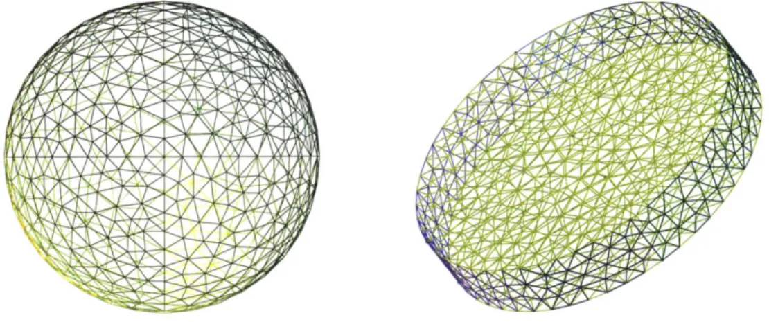
calized tangential-vector-valued basis functions that are restricted to the surface of the object. It is common to use basis functions that are defined over small triangular elements that approximate the surface of the object. Two examples of this type of surface discretization can be seen in Figure 2-1.

The restriction of currents to the surface is made without loss of generality using the well-known equivalence principle of electromagnetism, which states that the fields within the object can be completely specified by a fictitious distribution of source currents that are confined to the boundary

[23].

In other words, the BEM involves computing "effective" electric and magnetic surface currents that are mathematically equivalent to the volume currents that would be realistically flowing through the body. In Chapter 4, we will utilize a specialized piece of BEM software known as

SCUFF-NEQ to simulate thermal self-propulsion in a variety of different nanoparticle

configurations using precisely the trace formulas (2.26) that we have derived above.

-7

w

Figure 2-1: Typical triangular-element surface discretization scheme that is used in conjunction with the boundary element method.

Chapter 3

Fundamental Limits On Thermal

Self-Propulsion

Before we dive into the realm of computer simulation, there is a great deal of nu-merical and phenomenological insight to be gained from the scattering matrix theory that we described in Section 2.3. In this chapter, we will make use of the T-matrix trace formulas (2.27) and (2.28) to obtain fundamental limits on the thermal power emission and self-propulsion force that is attainable for particles of a given size. The most important result of this chapter is a set of explicit predictions-reported in Table 3.4 on page 43-for the maximum self-propulsion force that is attainable for

any homogeneous dielectric nanoparticle of arbitrarily complex shape. In addition,

we will explore details of the T-matrix formalism which, in this context, will allow us to extract useful design principles that will guide our numerical search for efficient self-propulsion geometries in Chapter 4.

We will restrict our attention to contributions to the power and self-propulsion force coming from photons emitted by the body at a single frequency. This approach has obvious limitations, but will not significantly reduce the generality of our results. We will demonstrate in Chapter 4 that the power and self-propulsion force are dom-inated by contributions coming from a small set of frequencies, particularly those associated with dielectric resonances. As long as we tailor our results to the resonant frequencies that are unique to each object, we will reap the benefits of reduced math-ematical complexity and computation time with only a minimal loss of predictive power.

the following simplified form: P=_ - _ <D,(W) d, (3.1) F oj{ ekBT l}

/0

2 hw 4D, . (3.2) fo 7r e kBT _ C

In these expressions, we have introduced the dimensionless quantities <D, and <PF representing the temperature-independent power flux spectral density

<D,~(W) = Tr 1(T + TV) - TV ,(3.3)

and force flux spectral density

=D w Jm Tr

I 5T7'}

(3.4)

where j = (w/c)- 1p is a non-dimensionalized version of the infinitesimal translation

matrix and the dependence on angular frequency w enters implicitly through the T-matrix. For the remainder of this chapter, we will work directly with (3.3) and (3.4), recognizing their unique dependence on particle shape and composition. For ease of discussion, we also will refer to (3.3) and (3.4) as the "power" and "force", respectively. It is our hope that any discomfort caused by our loose terminology will be alleviated

by the notable absence of the phrase "flux spectral density" in every sentence for the

remainder of the chapter.

Turning our attention to the form of these equations, we see that the force and the power both depend quadratically on the T-matrix. This quadratic dependence follows from the fact that the microscopic current densities in the radiating body enter into the formalism twice: once as the source of the incident field and again as the currents induced by the incident field. Due to the presence of an overall minus sign, the power (3.3) is a concave function of the elements of the T-matrix. This has the interesting consequence of ensuring the existence of a T-matrix that globally maximizes the emitted power. We will explore this feature analytically and discuss its physical significance in Section 3.1. The expression for the self-propulsion force (3.4) is complicated by the presence of 5, which mixes the T-matrix elements in a non-trivial way. It is unclear from the form of equation (3.4) alone whether the force magnitude has a finite upper bound. We will demonstrate in Section 3.2, however, that a global maximum force emerges when we impose constraints on the T-matrix

to ensure that it is physically realizable.

3.1

Upper Bound on Thermal Power Emission

Computing the T-matrix that globally maximizes the emitted power turns out to be a straightforward exercise in multivariable calculus, with the only complication arising from the fact that the elements of the matrix are complex numbers. We proceed by defining the elements of the T-matrix T3 in terms of their real and imaginary parts:

To = XQ + iya, T = T*3=a Xa - iyo, Xa,Yaa e R . (3.5)

Substituting (3.5) back into our expression for the emitted power (3.3) and simplify-ing, we arrive at the following equivalent expressioni:

(X) = - Tr{X + XXT _{+ yyT}. (3.6)}

In anticipation of computing the gradient, we re-express (3.6) in the form:

'Ip(X,

Y) = -Xaa - xaoxao - yaoyao) (3.7)

where we have made use of the convention that each repeated index is summed over all possible values2_.

Before we proceed, we should clarify what is meant when we speak of computing the "gradient" of (3.3). We have written the emitted power in the form (3.7) to emphasize the fact that the trace formula (3.3) is merely a multivariable function that maps complex "vectors" of length (dim T)2 _{[or two real "vectors" of length (dim T)}2_] into real numbers. In this language, the meaning of the gradient becomes clear: we are computing the sensitivity of the emitted power (3.3) to changes in the individual elements of the T-matrix, treating the real and imaginary parts of each element as distinct real variables. Now that the meaning is clear, the actual computation of the 'Moving forward, we will omit the implicit dependence on w from our expressions for power and force. For our purposes, it will suffice to think of these quantities as functions of the T-matrix elements alone.

2_{To make the meaning of (3.7) absolutely clear, we repeat it here with the implied summations} re-inserted:

gradient of (3.7) is quite simple:

aip = - ,ca va - 2 15a6v ,3X a ,3= - o - MX n , _(3.8)

& Dy _ - 2 6lia6v ,Y aO = 2Y qv . _(3.9)

Setting the gradient equal to zero and solving for X, and Yu, we obtain:

8x

-13

VX21V 2

a = 0 Y7V = 0,

which tells us that the T-matrix which maximizes the emitted power is given by:

-v = 216OV . (3.10)

Plugging this expression for the T-matrix (3.10) back in to the emitted power formula

(3.3) and recognizing that aa = dim T, we arrive at the following analytic expression:

max _P = dim T. (3.11)

4

This formula (3.11) highlights one detail of the T-matrix that we have, as of yet, glossed over. As an abstract mathematical object, the T-matrix is infinite-dimensional, so our formula (3.11) predicts that the maximum power should be infinite. We should not despair, however, as there is a subtle but important physical assumption lying beneath this conclusion.

To understand the significance of this subtlety, it will help if we fix in our minds a particular basis for the T-matrix. For the purposes of this discussion, the spherical basis will be the most intuitive, so moving forward we will imagine that all fields under consideration have been projected onto a basis of vector spherical wave func-tions3_{. In this case each entry of the T-matrix, written Tpim,p'e'm', represents the} complex amplitude of an outgoing vector spherical wave Eo"' with polarization P and multipole order

(f,

m) that is produced when the object under consideration is

illuminated by a regular vector spherical wave ETm, with unit amplitude. In this basis, we can formally write down an expression for the dimension of the T-matrix,

3

For a review of the definitions and properties of vector spherical wave functions, we refer the reader to any one of the following wonderful references on the topic [1, 11, 20].

as it is simply the total number of vector spherical multipoles:

dim T = 2 (2e+ 1). (3.12)

f=1

Thinking now in terms of spherical wave functions, it is easier to see the physical assumption being made in our expression for the maximum-power T-matrix (3.10): it describes an object that couples equally to spherical multipoles fields of arbitrar-ily high order. We now present a heuristic argument that demonstrates why this idealization can never be realized in practice.

3.1.1

Accounting for Particle Size

In Figure 3-1, we depict a two-dimensional slice of an arbitrarily-shaped particle of radius R that is in the presence of an incident field {Einc, Hinc} that is traveling with

wave vector k. As we can see, the particle is not assumed to be spherically symmetric, so the "radius" of the particle is meant to indicate the radius of the smallest sphere that can completely contain the object within its interior. Vector spherical harmonics of order f exhibit oscillations in the azimuthal coordinate 0 with period T~ 2i/fe.

For the incident field to excite spherical modes of order f within the particle, the wavelength A = 27r/k = 2wc/w must be less than the distance RAO over which the

material and geometric properties of the particle vary, which in turn must be smaller than the distance scale TR set by the period of the spherical mode. This length scale comparison allows us to make a rough estimate fmax of the largest spherical mode that can be supported in our particle's interior:

A < RAO < 2rR max = [wR . (3.13)

In equation (3.13), we have made use of the floor function

Lx],

which returns the largest integer that is less than or equal to x. In other words, any spherical modes of order f > emax that are excited in the particle will rapidly decay, meaning that their contribution to the scattered field will be negligibly small. We can now understand why our prediction for the maximum emitted power was unphysical: an object can only emit an infinite amount of power if it is infinitely large. For compact objects of radius R, however, there is a well-defined upper limit to the amount of power that can be emitted by photons with angular frequency w.

R

IEinc n

H k

Figure 3-1: Arbitrarily-shaped particle of radius R along with a rough estimate of the angle AO over which the shape of the particle varies.

multipole bound (3.13) into the language of T-matrices. By saying that the incident field in Figure 3-1 does not excite spherical modes of order f > fmax within the particle, we are claiming that spherical vector waves of order f > emax pass right through the

particle without even "seeing" it. Recalling the physical interpretation of Tim,p'e'm', we can see that this conclusion is equivalent to the requirement that all elements of the T-matrix with f and f' greater than emax be equal to zero:

Tpjm,ptym, ~ 0 for f, ' > fmax . (3.14)

With this condition (3.14), our expression for the maximum-power T-matrix (3.10)

is modified to read (in the spherical basis):

- I 4'Af6mim e, ' < emax

Tpfm,p'e'm, = 2 . (3.15)

0 otherwise

Plugging this modified T-matrix (3.15) back into the trace formula for emitted power (3.3), we obtain the same result that we had before (3.11), except that dim T is re-interpreted as the dimension of the non-zero portion of the T-matrix. Fortunately, this

is precisely what we get when we truncate the sum (3.12) at f = fmax. Computing

the partial sum and plugging (3.13) in for emax, we arrive at the following simple

expression for the maximum power that can be emitted at angular frequency w by an object of radius R:

<) max(w R) = [wR + 1 -1 (3.16)

3.1.2

Implications for Particle Design

We have obtained an upper bound on the thermal power emission for compact objects

(3.16), but can we design a particle that will achieve this maximum? In other words,

can we design an object whose T-matrix is given by (3.15)? This type of problem, known in the scattering literature as inverse design, is normally very difficult to solve. Luckily, however, the form of the maximum-power T-matrix is simple enough to permit a solution without much work. Here we will find it helpful to describe the particle by its S-matrix

135],

which is related to the T-matrix by

S = I+ 2T, (3.17)

where I is the identity matrix. The S-matrix provides a subtly different viewpoint by telling us how incoming vector spherical waves Eietm, transform into outgoing vector spherical waves E"t when they scatter off of the particle. According to (3.17), the maximum-power S-matrix is given by:

0 f, f' < max

Spem,pijm' = (3.18)

1 Pppfvfomn otherwise

The interpretation of the S-matrix is more straightforward: the particle described

by (3.18) absorbs all incoming spherical waves of order f < max but is otherwise

transparent. In the limit as max -+ oo, this S-matrix describes an idealized perfect

absorber, which is commonly referred to as a blackbody. A well-established corollary of Kirchoff's law of thermal radiation states that an object in thermal equilibrium with its surroundings will emit and absorb electromagnetic radiation at the same rate

[36].

In our case, this means that our perfect absorber will also be a perfect emitter4. In essence, we have rediscovered the fact, known to Kirchoff over 150 years ago, that-at a given temperature and frequency-a blackbody will emit more radiant energy than any other object held at the same temperature.

Another interesting facet of the blackbody emitter is that it radiates photons isotropically, so it will not exhibit thermal self-propulsion. After all, for an object to experience self-propulsion, there must be a directional imbalance in the linear

4_{In Chapter 4, we will study particles that are held at room temperature (~ 300 K) in vacuum. In}

this case, the warm particles are most definitely not in thermal equilibrium with their surroundings. This interpretation will still be valid, however, as we will only compute quantities in the instant of time after the particle is placed in vacuum and will assume that it was in thermal equilibrium with a heat source immediately before.

momentum that is leaving the body. It turns out that this attribute, which follows directly from the definition of a blackbody, is already encoded in the diagonal form of the maximum-power T-matrix (3.10). We will discuss the symmetry properties of the T-matrix in greater detail in Section 3.2.2, but for now it will suffice to know that an object whose T-matrix is diagonal in the spherical basis will exhibit spherical symmetry. In Section 2.3, we mentioned briefly that the infinitesimal translation matrix fp is purely off-diagonal. By simple calculation, one can show that the trace of the product of a diagonal matrix with a purely off-diagonal matrix is always zero, which is sufficient to conclude that the self-propulsion force (3.4) for a spherically symmetric particle will vanish.

This conclusion has interesting consequences with regard to the design of optimal propulsion geometries. For example, one might naively expect that the best self-propulsion design is a particle that emits all of its photons in a single direction. It is true that, if we fix the total power emitted by the body, then unidirectional photon emission, being maximally asymmetric, will result in the largest self-propulsion force. This is not, however, the design problem we face in reality. To understand why, let us consider first what would happen if we tried to work toward this goal with an actual particle that is composed of a fixed amount of dielectric (or conducting) material. We might start by molding our particle into the shape of a sphere, since have we just learned that this shape will give us the greatest power emission that is available to us. We will then proceed to deform the particle in some asymmetric fashion, with the intent of concentrating photon emission in a certain direction. What we will find, however, is that the further our particle deviates from spherical symmetry, the lower its total power output will be5_{. Therefore, there is a significant trade-off that occurs} between our ability to increase the concentration of photons in a particular direction and the total number of photons available to us. In other words, even if we were to somehow design a particle that emitted all of its photons in a single direction, the total power that would be emitted by the object would be quite low, suggesting that there is some less geometrically extreme particle that would perform better.

3.2

Upper Bound on Thermal Self-Propulsion

We now wish to use the techniques we have developed and the insight we have gained in the previous section to compute the maximum thermal self-propulsion force that

5

This must be the case, since any deformation that moves the particle toward spherical symmetry will increase the emitted power.

can be achieved by a particle of radius R that is emitting photons with angular fre-quency w. As we anticipated in the chapter introduction, this problem is significantly more difficult than the one we encountered in Section 3.1, for a number of reasons. First of all, we must now contend with the infinitesimal translation matrix ], or, p-matrix for short. The complexity of the p-matrix is reduced considerably when we work in the spherical basis and restrict ourselves to self-propulsion forces along the z-axis; however, it is still formidable and will make calculations involving the force and its gradient more laborious. Secondly, we will discover that if we naively attempt to compute the maximum force by setting the gradient of (3.4) equal to zero and solving for the elements of the T-matrix, we will obtain a T-matrix that does not correspond to a physically realizable particle. As it turns out, there are additional symmetries and properties of the T-matrix that must be satisfied for our upper bound to be meaningful. In our maximum-power calculation, these conditions were automatically satisfied due to the diagonal, spherically symmetric form of the solution. In the realm of force calculations, we no longer have the luxury of a simple T-matrix, and must therefore devise a strategy for imposing the extra constraints. Finally, there is no reason a priori to believe that a closed-form, analytic expression for the maximum force T-matrix even exists. With all of this in mind, we will focus our efforts on molding this problem into a form that can be efficiently be handled by NLopt, an open source library for nonlinear optimization

[14].

3.2.1

Computing the Gradient

Although it is not strictly required, many of the nonlinear optimization routines that are available to us can be sped up dramatically by supplying an analytic formula for the gradient. This eases the computational burden by reducing the total number of times that the objective function (3.4) must be evaluated while the search for a maximum is conducted. We will again define T and Tt according to (3.5), and we will decompose the p-matrix in a similar way:

Paf =QPaa + iQa , Pcp , Q,, cE R . (3.19)

Before moving on, it is important to reiterate that despite their complicated origin, the matrices P and Q are strictly constant, and will simply be carried along in our computation of the gradient. With this mind, we can plug (3.19) and (3.5) into the

original expression for the force (3.4) to obtain:

DF(X, Y) = T- (3.20)

Following the steps we took in Section 3.1, we write (3.20) in component form:

(DF(X, Y) = PaYO-yXa-j + QaOX,3yXay - Po~X)3yY + Qay,Y6YcY.- (3.21)

At this point, computing the gradient of (3.21) is simply a matter of applying the product rule and keeping close track of indices. The result is given by the following two expressions:

- (Q77 + Q Q?l)XQv + (P77 - -Pa(3.22)

-YJ -(P~l - Pca)Xav + (Q77a + Qa??)Ycw.

(3.23)

3.2.2

Symmetries of the T-Matrix

Few techniques in the scattering theorist's arsenal match the versatility, accuracy, and elegance of the T-matrix. We have seen evidence of its symbolic power: equa-tions (3.1) and (3.2) hold true for any object that one could imagine. However, the simplicity and compactness of these formulas can be quite misleading. It is true that all of the mathematical difficulties that arise when dealing with realistic materials and geometries have been abstracted away, but they certainly have not disappeared from the calculation. They have merely been reassigned to the poor soul in charge of computing the elements of the T-matrix. For those of us who must, for one reason or another; "look under the hood" and grapple with the elements themselves, the T-matrix can seem rather intimidating. Working in the spherical basis and retaining only elements corresponding to the lowest-order mode, the T-matrix is composed of

36 complex numbers that collectively describe the geometric and material features of

the object that can be resolved by

e

= 1 spherical waves. If we add in the fact that

the number of elements in the T-matrix grows like (fMax + 1)4, it may sound enticing

to abandon our efforts before they've even begun. Fortunately, however, the elements of the T-matrix are not all independent.

We have collected in Table 3.1 a short list of symmetry properties of the T-matrix in the spherical wave basis

119].

The first property in our list must be satisfied in

6

In the engineering literature, this property is said to follow from electromagnetic reciprocity [19]. Reciprocity, however, is a direct consequence of the time-reversal invariance of Maxwell's equations.

Table 3.1: An (incomplete) collection of T-matrix symmetry properties that hold in the spherical wave basis 1191.

any system that is symmetric under a reversal of the direction of time. The theory of electrodynamics, as described by Maxwell's equations, is completely unchanged by the transformation t -+ -t, so we must take care to ensure that this property holds in any T-matrix that we claim maximizes self-propulsion force. Knowing this ahead of time, we can pre-program this symmetry property into the T-matrix by restricting the space of possible matrices that our nonlinear optimization software can explore. We are also free to restrict this space further by requiring that our particle exhibit spatial symmetries. Looking at the second property in our list, we see that one can ensure azimuthal symmetry by setting all T-matrix elements with m -, m' equal to zero, and we will find it advantageous to do so. As we discussed in Section 3.1.2, thermal self-propulsion forces are a result of asymmetric photon emission. Imagining a coordinate system whose origin lies at our particle's center of mass, it stands to reason that self-propulsion forces directed along the z-axis arise when our particle is asymmetric under reflections about the x - y plane. It is clear, then, that the requirement of azimuthal symmetry neatly confines our particle to motion along the z-axis. It is also clear from this line of reasoning that our space of possible T-matrices should not include those that satisfy properties three and four in our list7.

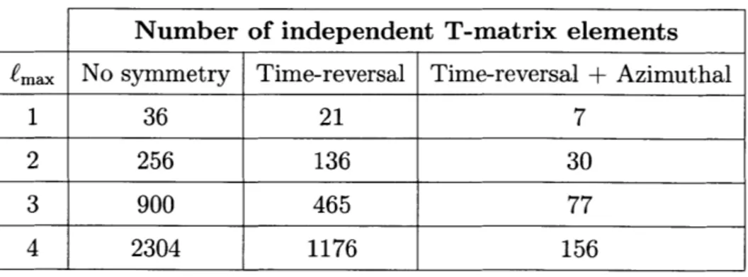
A quick glance at Table 3.2 will reveal that by requiring that our particle be

azimuthally symmetric and time-reversal invariant, we have dramatically reduced the number of independent T-matrix elements. The addition of azimuthal symmetry comes with the auxiliary benefit of setting a large number of independent elements equal to zero. We can directly exploit the sparsity of our T-matrix in costly linear

7_{Property four in Table 3.1, which is simply a combination of properties two and}

three, was discussed in detail in Section 3.1.2.

Symmetry T-Matrix Property

Time-reversal6 TPem,P'em' = ( -1)mm'7p,,,p,_m

Azimuthal Tpem,p',tm' = 6m'mTfm,p'e'm

Reflection: x - y plane TPm,Pem' = 0 unless (_ J+f

= I

Tpipme/m, = 0 unless (- 1)'+" = -1 Spherical Tpmpe',m' = 6p'p6e' 6mmTpim,pem

Table 3.2: List of the number of independent elements in T-matrices that satisfy various symmetry properties.

algebra operations to achieve a substantial reduction in computation time. At this stage, we appear to be in pretty good shape. We have worked hard to ensure that our particle is not engaging in egregious violations of physical law, and have reduced the computation time for our optimization problem from weeks to hours. However, if we were to attempt the computation now, we would find that the optimizer would return infinity. There is one more condition that the T-matrix must satisfy to ensure that it is physically realizable, and it turns out that imposing this condition efficiently is rather difficult.

3.2.3

Conservation of Energy

As it stands, there is nothing stopping our nonlinear optimization software from sending all of the independent elements of the T-matrix to infinity. Let us use the S-matrix to consider the physical implications of this process. As we have mentioned before, the elements of the S-matrix represent the complex amplitudes of outgoing spherical waves that result from incoming spherical waves with unit strength. These complex amplitudes provide us with the expansion coefficients of the scattered field. We can use the magnitude of the scattered field coefficients to compute the Poynting vector, which, when integrated over any surface that completely encloses the object, tells us the rate at which energy is being carried off to infinity. It is clear, then, that if we multiply the T-matrix by a number that is greater than one, we will increase the total amount of energy that is leaving the body per unit time. Since the amplitude of incoming waves is fixed at unity, there is surely a point at which the rate of energy leaving the body will exceed the rate of energy that is being supplied. An object with this property is said to be an active or gain medium, and generally relies on an external power source to achieve field amplification.

Number of independent T-matrix elements

emax No symmetry Time-reversal Time-reversal + Azimuthal

1 36 21 7

2 256 136 30

3 900 465 77

In contrast, the particles that we are interested in consist of passive or lossy media. Each particle constitutes an isolated physical system whose only source of energy comes from thermal current fluctuations. In this case, it is obvious that there must be an upper bound to the rate at which energy (and momentum) can leave the body. How, then, is this bound encoded in the properties of the S-matrix? It turns out that the statement of conservation of energy is equivalent to the requirement that the matrix I - SSI be positive semi-definite 119]:

I - SSt > 0. (3.24)

Although it's not immediately obvious, this condition (3.24) ensures that the S-matrix maps all non-zero vectors into vectors with a smaller Euclidean norm8. This statement is precisely what we had in mind when we discussed using the S-matrix to compute the Poynting vector. We can now use equation (3.17) to derive an alternative expression of energy conservation in terms of the T-matrix:

2 (7T + V) - TVf > 0 .(3.25)

We can see immediately that (3.25) places a condition on precisely the same matrix whose trace gives us the emitted power (3.3).

At long last, our final task has emerged. In order to compute a physically mean-ingful upper bound on the thermal self-propulsion force that can be attained by a compact object emitting photons with angular frequency w, we must perform a nu-merical optimization of the force (3.4), subject to the constraint that the T-matrix is azimuthally symmetric, time-reversal invariant, and that a particular nonlinear func-tion of the T-matrix (3.25) is positive semi-definite. As we discussed in Secfunc-tion 3.2.2, symmetries of the T-matrix are easily enforced by restricting the space of possible matrices that our optimization software can explore. Efficiently imposing the positive semi-definiteness constraint (3.25), however, will bring us to the forefront of applied mathematics.

Semidefinite programming (SDP) is a rich and exciting field of applied mathe-matics that has primarily developed in the past twenty years [7]. The objective of

linear SDP is to minimize a linear function F(M) -+ R subject to the constraint that the matrix M > 0. It was demonstrated in the 1990's that linear SDP is

ef-8_{To understand why this is true, consider the following alternative statement of (3.24):} xt (I - StS) x > 0 for all complex vectors x. By simple linear algebra manipulations, one can