Complex materials handling and assembly systems.

COMPLEX MATERIALS HANDLING AND ASSEMBLY SYSTEMS Final Report

June 1, 1976 to July 31, 1978

Volume V

ALGORITHMS FOR A SCHEDULING APPLICATION OF THE ASYMMETRIC TRAVELING SALESMAN PROBLEM

by

Paris-Christos Kanellakis

This report is based on the unaltered thesis of Paris-Christos Kanellakis, submitted in partial fulfillment of the requirements for the degree of Master of Science at the Massachusetts Institute of Technology in May,

1978. This research was carried out at the M.I.T. Electronic Systems

Laboratory with partial support extended by the National Science Foundation grant NSF/RANN APR76-12036. (A few copies of this report were previously distributed under the number ESL-TH-823.)

Any opinions, findings, and conclusions or recommendations expressed in this n publication are those of the authors, and do not necessarily reflect the views of the National Science Foundation.

Electronic Systems Laboratory Massachusetts Institute of Technology

OF THE ASYMMETRIC TRAVELING SALESMAN PROBLEM by

Paris-Christos Kanellakis

S.B., National Tech. Univ. of Athens, Greece, (1976)

SUBMITTED IN PARTIAL FULFILLMENT OF THE REQUIREMENTS FOR THE DEGREE OF

MASTER OF SCIENCE at the

MASSACHUSETTS INSTITUTE OF TECHNOLOGY May 1978

Signature of Author... ...

Department of Electrical Engineering and Computer Science, May 24, 1978

Certified by ... ...

Thesis Supervisor

...

'...

...

Thesis Supervisor

Accepted by ... ... Chairman, Department Committee on Graduate Students

by

Paris Christos Kanellakis

Submitted to the Department of Electrical Engineering and Computer Science on May 24, 1978, in Partial Fulfillment of the Requirements for the

Degree of Master of Science.

ABSTRACT

We examine the problem of scheduling 2-machine flowshops in order to minimize makespan, using a limited amount of intermediate storage buffers. Although there are efficient algorithms for the extreme cases

of zero and infinite buffer capacities, we show that all the intermediate (finite capacity) cases are NP-complete. We analyze an efficient approxi-mation algorithm for solving the finite buffer problem. Furthermore, we show that the "no-wait" (i.e., zero buffer) flowshop scheduling problem with 4 machines is NP-complete. This partly settles a well-known open

question, although the 3-machine case is left open here. All the above problems are formulated as or approximated by Asymmetric Traveling Salesman Problems (A-TSP). A methodology is developed to treat (A-TSP)'s.

Thesis Supervisor: Ronald L. Rivest

Title: Associate Professor of EECS Thesis Supervisor: Michael Athans

Title: Professor of EECS, Director ESL

-2-I would like to express my sincere thanks to Prof. Christos H. Papadimitriou of Harvard for his help and collaboration that made this

research possible. I am greatly indebted to Prof. Ronald L. Rivest who supervised this work with great understanding and many helpful sug-gestions. I would also like to express my deep appreciation to Prof. Michael Athans, whose encouragement and constant support were invaluable.

Finally, I would like to thank Ms. Margaret Flaherty for the excellent typing of this manuscript.

This research was carried out at the M.I.T. Electronic Systems Laboratory with partial support extended by the National Science Foundation grant

NSF-APR-76-12036.

ABSTRACT 2

ACKNOWLEDGEMENTS 3

TABLE OF CONTENTS 4

CHAPTER 1: INTRODUCTION AND PROBLEM DESCRIPTION 6

1.1 Motivation 6

1.2 Problem Description 9

1.2.1 Discussion 9

1.2.2 The Finite Buffer Problem 10

1.2.3 The "No-Wait" Problem 14

1.2.4 The Significance of Constraints 20 1.3 The General Scheduling Model and Extensions 22 1.4 Notions from Complexity Theory and the Efficiency 24

of Algorithms

1.5 A Summary and Guide to the Thesis 28

CHAPTER 2: COMPLEXITY OF FLOWSHOP SCHEDULING WITH LIMITED 33 TEMPORARY STORAGE

2.1 The Two Machine Finite Buffer Problem - (2,b)-FS 33

2.2 The Fixed Machine "No-Wait" Problem - (m,0)-FS 41

2.3 Three Machine Flowshops 56

CHAPTER 3: AN APPROXIMATION ALGORITHM FOR TWO MACHINE FINITE 62 BUFFER FLOWSHOPS

3.1 The (2,0)-FS Problem and the Gilmore Gomory Algorithm 62

3.2 An Approximation Algorithm 66

3.3 Bounds for Flowshop Scheduling 73

3.4 The Significance of Permutation Scheduling 78 CHAPTER 4: THE ASYMMETRIC TRAVELING SALESMAN PROBLEM 88

4.1 Neighborhood Search Techniques and Primary Changes 88 4.2 The Significance of the Triangle Inequality 98

4.3 A Proposed Heuristic 102

-4-TABLE OF CONTENTS (con't)

Page

CHAPTER 5: CONCLUSIONS AND OPEN PROBLEMS 108

APPENDIX 110

1.1 Motivation

"What do I do first?" _{This irritating question has tormented us} all. _{It has plagued the student in his thesis, vexed the engineer in} his design, and worried the technician in his workshop. It is bound to puzzle any machine that aspires to be versatile and efficient. The auto-matic factory will have to live with it and above all answer it. What

is most annoying is that it is never alone, but has a demanding sequel "What do I do next?"

In very general terms, that is the fundamental question the theory of scheduling set out to answer a quarter of a century ago. Because of its applicability to diverse physical systems as jobshops or

com-puters, this theory spans many powerful disciplines such as Operations Research and Computer Science. Therefore it is not by chance that the ideas used in the present work were provided by the theory of Algorithms and Complexity.

Scheduling follows such functions as goal setting, decision making and design in the industrial environment. Its prime concern is with operating a set of resources in a time- or more generally cost-wise efficient manner. _{The present work was motivated by a number of} ob-vious but significant facts about the operation of highly automated shops with multipurpose machines for batch manufacturing (e.g., a job-shop with computer controlled NC machines and an automated materials handling system). Let us briefly look at these facts:

-6-(a) A large percentage of the decisions made by the supervisor or the computer control in such systems are scheduling decisions. Their objective is high machine utilization or equivalently schedules with as little idle time and overhead set-up times as possible. Therefore any analytic means to decide "what to do next?" with a guarantee of good performance will be welcome.

(b) Well behaved mathematical models (e.g., queueing models or network flow models) tend to appear at aggregate levels. Yet scheduling decisions are combinatorial in nature. A combinatorial approach can be useful both in the insight it provides and the determination of power-ful non-obvious decision rules for giving priorities to different jobs. By making simplifying assumptions (e.g., replacing a complicated trans-fer line with a fixed size buftrans-fer) we can sometimes get a tractable combinatorial model.

(c) The trend in the hardware design is towards few powerful machines (typically 2 to 6) set in straight line or loop configurations with storage space and a transfer system. What is significant is the small number of machines, usually small buffer sizes (1 or 2 jobs in metal cutting applications) and the simple interconnection. The con-figuration studied consists of the machines in series (flowshop) under the restriction of finite buffers between machines (Figure 1). This does not give us the full job shop freedom of the transfer line as in

(Figure 2). Yet let us look at an abstraction of the system in Figure 2. Consider a series of machines with buffers in between (which model the actual storage and the storage on the transfer line). The jobs

1 2 m

Buffer

Figure 1

PQueue

Transfer Line

Ml

M14

_{rLoading & Unloading Stations}

Figure 2

Bujfer |

Mli

_4ii

_[

_F

_3I

M4

(Figure 3).

Decidedly Figure 3, because of communication between buffers,

is more complicated than Figure 1, which is a necessary first

approxi-mation.

(d) Scheduling models might sometimes look too simple, also the

jobs are not always available when we determine the schedule. All this

can be compensated by the fact that computers are much faster than other

machines and we can experiment with simulation and heuristics (that the

theory provides) long enough and often enough to make good decisions.

Let us now proceed with a detailed description of our scheduling

problem, its setting in the context of the general scheduling model,

the central ideas used from the theory of Algorithms and a brief look

at the results obtained.

1.2

Problem Description

1.2.1 Discussion

We examine the problem of "scheduling flowshops with a limited

amount of intermediate storage buffers".

Flowshop scheduling is a problem that is considered somehow

inter-mediate between single- and multi-processor scheduling.

In the version

concerning us here, we are given n jobs that have to be executed on a

number of machines. Each job has to stay on the first machine for a

prespecified amount of time, and then on the second for another fixed

amount of time, and so on. For the cases that the (j+l)st machine is

busy executing another job when a job is done with the j-th machine,

the system is equipped with first-in, first-out (FIFO) buffers, that

cannot be bypassed by a job, and that can hold up to b. jobs at a time

(see Figure 1). We seek to minimize the makespan of the job system, in other words, the time between the starting of the first job in the first machine and the end of the last job in the last machine.

Two are the significant cases studied here:

(i) 2-machine flowshops with finite intermediate storage of size b > 1.

(ii) m-machine flowshops with no storage at all, where m is a fixed number larger than two; (also known as

"no-wait" or "hot-ingot" problem.)

Apart from their practical significance, for which we argued in section 1.1, these problems are important because they are the simplest in the hierarchy of flowshop problems (see Figure 10), whose complexity the goal of this work was to study. Particularly problem (ii) can be formulated as an Asymmetric Traveling Salesman Problem (ATSP - given a directed graph and a weight function on the edges, find a path visiting all vertices exactly once at minimum cost). Let us now formulate our problems in a more rigorous manner.

1.2.2 The Finite Buffer Problem

We start by introducing (i). Each job is represented by two positive* integers, denoting its execution time requirements on the first and second machine respectively. Now, a feasible schedule with.

*For the purpose of clarity in the proofs that follow, we also allow 0 execution times. If a job has 0 execution time for the second machine it is not considered to leave the system after its completion in the first machine. One may disallow 0 execution times, if they seem

un-natural by multiplying all execution times by a suitably large interger --say n -- and then replacing 0 execution times by 1.

b buffers is an allocation of starting times to all jobs on both machines, such that the following conditions are satisfied:

a) No machine ever executes two jobs at the same time. Naturally, if a job begins on a machine, it continues

until it finishes.

b) No job starts on any machine before the previous one

ends; no job starts at the second machine unless it

is.

done with the first.

c) No job finishes at the first machine, unless there is

buffer space available ---

in other words there are

less than b other jobs that await execution on the second

machine.

One may allow the use of the first machine as

temporary storage, if no other buffer is available; this

does not modify the analysis that follows.

In Figure 4

it is demonstrated that this is different from having

an extra buffer.

d) All jobs execute on both machines in the same order;

this restriction comes from the FIFO, non-bypassing

nature of the buffer.

More formallly,

DEFINITION. A job J is a pair (a,f) of positive integers. A

feasible schedule with b buffers for a (multi)-set

J

= {J ,...,J

}

-1 n

of jobs (called a job system) is a mapping S:{l,...,n} x {1,2}

+

N;

S(i,j) is the starting time of the i-th job on the j-th machine.

(The

finishing time is defined as F(i,l) = S(i,l) + i.,

F(i,2) = S(i,2) + i.

)

S is subject to the following restrictions

a) i f j + S(i,k)

$

S(j,k).

b) Let 71' 72 be permutations defined by i < j + S(Tk(i),k) < S(Ok(j),k). Then

T

1 = 72 = v (this is the FIFO rule).

d) F( (i),l) < S(T(i),2).

e) i > b + 2 + F(r(i-b-1),2) < F ((i),l)*.

The makespan of S is p(S) = F(r(n),2). It should be obvious how the definition above generalizes to m machines.

A feasible schedule is usually represented in terms of a double Ghannt chart as in Figure 4. Here 5 jobs are scheduled on two machines

for different values of b, r is the identity permutation. In 4a and 4c a job leaves the first machine when it finishes, whereas in 4b and 4d it might wait. The buffers are used for temporary storage of jobs (e.g., job (3) in 4c spends time T in the buffer). A schedule without superfluous idle time is fully determined by the pairs (ai, i), r and b; hence finding an optimum schedule amounts to selecting an optimum permutation.

Some information had been available concerning the complexity of such problems. In the two-machine case, for example, if we assume that there is no bound on the capacity of the buffer (b = -) we can find the optimum schedule of n jobs in O(n log n) steps using the algorithm of

[20]. Notice that, for m > 2, the m-machine, unlimited buffer problem is known to be NP-complete** [13]. Also for two machines, when no

buffer space is available (b = 0, the "no-wait" case) the problem can be

* If we assume that the first machine acts as temporary storage the only modification is that e) becomes

i > b + 2 + F(OT(i-b-2), 2) < S(QI(i), 1)

**

See Section 1.4,characterizing the problem as NP-complete means that it is essentially computationally intractable.

,

,

2

2

3

3

Mach

I2

1

3

4

2

3

3

3

1 i i i - I

4

t

I

0

2

3

4

5

7

8

9

1

time

i

5

2

2

(o)

I

~

2

3

V~A

4

345

1

Y~1

2

34

V34

5

~o

ti(b)

tt

I 1

2 3

4 5

Figure 4

4

5

a) b=O

0

(C)

14---r

tO10

c) b=l

d) b--=lO

₂

₃

0

(d

2

3

4

15

0

(d]

tO

considered as a single-state machine problem in the fashion of [10], As noted by [11], the case of the 2-machine flowshop problem in which b is given positive, finite integer was not as well understood. In fact, in [9

1

this practical problem is examined, and solutions based on dyna-mic programming are proposed and tested.

Although there are efficient algorithms for the extreme cases of zero and infinite buffer capacities, all the intermediate cases (.finite capacity cases) are NP-complete. We analyze an efficient heuristic for solving the finite capacity problem.

1.2.3 The "No-Wait" Problem

Let us, now take a look at problem (ii) of 1.2.1. We present re-sults that extend our understanding of the complexity of flowshop scheduling under buffer constraints in another direction: we show that the m-machine zero-buffer problem is NP-complete for m > 4. As mentioned earlier, the m = 2 case can be solved efficiently by using ideas due to Gilmore and Gomory [10] and such "no-wait" problems in general can be viewed as specially structured Traveling Salesman problems [32],

[33], [39]. Furthermore, it was known that the problem is hard when m is allowed to vary as a parameter [24]. For fixed m and particularly m = 3 the complexity of the problem was an open question [24], [18]. Although our proof for m > 4 is already very complicated, it appears that settling the m = 3 case requires a departure from our methodology.

We will demonstrate the connection between Asymmetric Traveling Saleman Problem (ATSP) and the scheduling problem by presenting the formulation of the "no wait" problem as a directed graph problem [33],

in this representation.

Each job is an m-tuple of numbers. We have the same restrictions

of flowshop scheduling as in 1.2.2, only now b = 0 and m > 2. Let tij

be the time to process job Jj on Machine Mi. Each job will correspond

to a node in the graph.

(We also have a start node with t

0 l<i<m).

The weights on the arcs (i,j) depend on the idle time on machine k,

l-<k<m, that can result if job Ji precedes Jj in the schedule.

Let us

call this idle time Ik(i,j).

We have [33]:

_ k-l

Il(i,j) = max

't

-

;

t

,j

0

2 < k < m i

k-l

k

I

k

(i,j) = I

l (i,j)

+

tT

j

-

tT

i 2

< k <

m

0 <

i,j

<n

1=1

T=2

There are k equivalent formulations as ATSP's with the distances

ex-pressing the idle times directly. Note that we have n+l nodes, where

the n nodes correspond to the n jobs and the n+l

s

t one to the starting

node with all processing times 0.

<

k <m ATSPk : Cij= Ik(i'j) 0 < i,j < n

If for simplicity the optimal permutation of jobs is the identity we

have:

n

(Optimal Schedule) =

EtkT

+ (Optimal tour of ATSP

k)

T=l

k

Vk

k

=

tk

+

C

ii+1

+Cno =

kl CO1 C ii+l nO

T=O T=1

n n

(i+l) mod(n +1) ki

E

(i+l) mod(n+l)

i=O i=O

n n

- k~i~l~mod~n~lI=

i(i(i+l)mod(n+l)+

i(i+l)mod(n+l) (**)

i=O i=O

wk kr k k

where d.j = C.. + tki p C.. + t

13 13 ki ij 13 kj

The TSP formulations based on the dkijs and the P ijs satisfy the triangle inequality. dk dk ij Pi p.kjk PXj _dk \ Figure 5 k k k k k k

di +d > d.. and Pix + P j > P. because:

d xj- ij

IX

Xj

- 1j

k k k

d. +

dXj

-

d.

.= Ik(i,X) + Ik(Xj) - Ik(i,j) + tk_i + tkX tki

ix 13 k k k ki kX ki

k k k

ik

+ PXj

i-P

(iX)

+ (Xij) Il(ij) +tlX = (by substitution)

K1 K--l K2 K2-1 -K K₃-1

T=

tTi _

+

TtTX -E

ti

T j t Ti

-

t T >

TT=1 T=1 T=1 = 1 T=

(by adding tli- tli and substituting)

(

K3 1

K

K 3-

The formulation commonly used is with

/k

k-l

d.. = max

t

-

t.

13 lJ<k<m Tt=l i T=l

Example: In order to illustrate the above let us formulate the ATSP1 for 2 machines and jobs (tli, t2i) = (ai,

Si

)

C.. = max (5. - '., O)

d.. =max (c. + 3. -c.,

Co.)

13 1

P.. = max (aj.,

.i)

For the ATSP1 for 3 machines and jobs (ai.

Si'

Yi) we have:

13 1 1 3 3 1 Cij = max (ai + Yi (j + j) i - j 0) 13 1 i 1

3

31

3 1 di max ( i +i -i (ej + Bj), c_i + _i .j' - i)

P.. = max (S. + Y. -

5.,

a.,

5.)

13 1 1 3 3

1

Note that in the first example all distances Pij are increased by an increase in the job lengths. In the second example an increase in the B's will increase some distances and might decrease others.

For the set of tasks

3

figure 6 has the ATSP2 formulation and figure 7 the Ghannt charts for schedules using 1 or 0 buffers.

Certain remarks are significant. First if we assume a formu-lation using idle times as distances and consider only the arcs with

0 weight, the existence of a Hamilton circuit (a circuit visiting all nodes exactly once) in the resulting graph indicates that there is a schedule saturating machine k. Second we actually have mn degrees

size b

Jobs

Machine

Machine

Product

1

/

D

1

2

(a) Two-machine flowshop with buffer size b

Time spent on

Time spent on

Job.

Machine 1 (t

l i

)

Machine 2 (t

2

i)

1

~

O

2

2

1

~0

2

2

2

12

3-

5

1

4

8

s 0

(b) A set of tasks '7

(0,0)

(2,12)

(5,1)

0

(0,2)

(8,0)-(c) The TSP, which corresponds to'Yand b

-

0. Optimal tour is in

heavy lines. The distances of the TSP are C..

C.. is the idle time on Machine 2, if job j follows job i

II

C q =

max

To.

I

t

til

C. =0

oJ

ii

CFigure

6=

cD

0

enters

_b~uffer

M2

t

2

5

7

10

14

15

Li.

1

leaves

buffer

(a)

The optimal schedule for

2"

if b

=

1.

The permutation of

jobs is ()-

(

-

)

M

2

0

DL(D

1

2

9

14 15

22

(b) The schedule for

the

permutation of

jobs

0

-

0

-

0

-

0

and b = O. [(a) is a compression of (b)]

0

,,

M

2 Q ILE 3

_

_

_

|

2

5

6

7

11

19

(c)

The optimal schedule for

Y'

if b = O. The permutation of

iobs s O

-

-

0

-0

of freedom to construct a matrix of (n+l)n distances which satisfy the

triangle inequality. If m is a parameter we can take m=O(n

2

) and expect

to come up with a problem as difficult as the general TSP.

This

in-tuition is correct [24].

If m is fixed the problem of determining its

complexity is more difficult.

1.2.4 The Significance of Constraints

Let us briefly comment on three issues related to the constraints

in our problem definitions.

1) If we assume that a machine can serve as temporary storage

this does not affect our analysis (e.g. increase b), and produces only

minor modifications in the schedule (see figure 4).

2) By accepting jobs of 0 length we do not assume that they can

bypass the machines or leave the system. This is in contrast with

[36], which treats the complexity of "no-wait" job-shops and

open-shops.

Also [36] introduces a "flow shop with 0 tasks".

Such a

dif-ference in definition (jobs able to bypass machines) makes it simple

to derive NP-completeness results from partition problems, but the

problem is no longer the "no-wait" fixed size flowshop problem [24].

3) In a flowshop of m machines and n jobs the combinatorial

opti-mization problem addresses the question of determining a permutation

of jobs to be performed on each machine (that is m permutations

I

l<i<m, such as those in the definition of 1.2.2).

Therefore the

1

--space of permutations that we must search is roughly 0((n!)m

). We

would like to be able to search a smaller space.

For all buffers

o

there are two classical results in scheduling theory [7 ], which

demon-strate that we can restrict our attention to equal permutations on the

first two machines and the two last ones (for a makespan criterion),

without loss of optimality. Since the problem is difficult anyway it

is customary to look only for some good schedule with the same

permuta-tion of jobs for all machines (optimal in the space of permutapermuta-tion

schedules).

This is obviously the correct approach when all buffers

are 0, yet it does not hold for b finite > 0. Even when b=l, m=2 we

might have a job bypassing another job that remains in the buffer and

allowing 71

t r2

our schedule might fare slightly better than under

the FIFO assumption. This is demonstrated in Figure 8 and more closely

examined in chapter 3. We conjecture that removing the FIFO assumption

results, at best, in negligible gains for the b = 1 case.

Job #

Ci

i

1

0

100

2

80

40

3

10

1

4

50

9

5

5

0

6

5

0

a

2

=

80

a

4

=50

a3=10

a=5 a5

,-

₁

00 -

₂

..

:40

P

₄

9

Figure 8

b=l 1TT=2

1.3 The General Scheduling Model & Extensions

In this section we will sketch the simple combinatorial model, which

defines most deterministic scheduling problems. This is done in order

to provide a complete view of the setting in which the present work fits.

Also this section provides us with a common language for problems

ad-dressed in chapters 2 and 5 or referred to elsewhere in this thesis.

Suppose that n jobs Jj(j=l,...,n) have to be processed on m machines

M.

(i=l,...,m). The most basic assumptions are that each machine can

process at most one job at a time and that each job can be processed

on at most one machine at a time. The scheduling problem has three

dimensions, which are more thoroughly examined in [18].

1) Resources:

We have m machines, wherem

might be fixed or a

problem parameter. We might have a single machine, identical, uniform

(they perform the same tasks at different speeds) or unrelated parallel

machines. Common network configurations are the flow-shop (defined in

1.2), the open-shop (each J. consists of a set of tasks one for each of

J

the m machines, but the order of execution is immaterial) and the

job-shop (each J. consists of a chain of tasks on a subset of the machines).

In general we also have a set of resources, which can be shared and

which are scarce

R = {R1 ... ,Rs} where Ri < Bi 1 < i < s

The buffer resources examined in this work can both be shared and form

part of the network topology of the system. Generally there seems to be

2) The Job Characteristics The jobs can be characterized by

a) Precedence constraints expressed as an irreflexive partial order on the tasks. This partial order < is represented by a directed acyclic graph, which in special cases can have the form of a tree or a set of chains (as in the flowshop case).

b) Processing times t.. > 0 of J. on M..

c) Resource requirements Ri (J.) < Bi of a job Jj

for resource i (B. = maximum available resource).

d) Release dates r., on which Jj becomes available and

due dates d., by which J. should ideally be completed.

If Fi(S) denotes the finishing time of a job in a

1

schedule S, then F.

(S)-d. is its lateness and

1 1

max{0O, F.(S)-d.} its tardiness.

3) Optimization Criteria

Our goal is to determine a sequence of tasks S such that certain

performance measures are optimized.

These optimal schedules might

be-long to general classes: preemptive, nonpreemptive (each task is an

entity and cannot be subdivided and executed separately), list scheduling

(a priority list is constructed and tasks are taken from it if the

proper processor is free and the precedence constraints satisfied),

permutation scheduling (in flow shops as discussed in 1.2.4) etc.

The

common performance measures are maximum finishing time

max (Fi(S)) or

l<i<n

makespan, mean weighted finishing time, maximum or mean weighted lateness

and tardiness.

In the last few years we have witnessed a spectacular progress towards understanding deterministic multiprocessor scheduling problems of various types. For an overview of results in scheduling we recommend

[5 ]; [11], [18] and [7

1

also stress certain aspects of the area. 1.4 Notions from Complexity Theory and the Efficiency of Algorithms

In order to investigate the computational complexity of a problem, the meanings of "problem" and of "computation" must be formally defined. We will attempt to illustrate these definitions.

A problem might be considered as a question that has a "yes" or "no" answer. Normally the question has several parameters, i.e., free variables. A selection of values for the parameters is termed an

in-stance of the problem. The size of the instance is the length of the string used to represent the values of the parameters. When we speak about complexity O(n3), n is the size of the instance.

The time needed by an algorithm expressed as a function of the size of the instance of the problem is called the time complexity of the algorithm. The limiting behavior of the complexity as size increases is called the asymptotic time complexity. Analogous definitions can be made for space complexity and asymptotic space complexity.

The theory of computation has created and analyzed simple computer models (automata) in order to determine the limits of computer capabili-ties and make precise the notion of an algorithm. This is where the study of time and space requirements on computation models (e.g., Turing machines, pushdown automata, etc.) has been fruitful. A distinct line

as those solvable efficiently or those that have polynomial time

com-plexity.

These easy problems belong to the class P. The other

inter-esting class for our purposes is NP (for nondeterministic, polynomial

time).

It encompasses P and all problems, which can be solved by a

nondeterministic Turing machine in polynomial time.

All problems in NP are solvable in principle, but for those whose

status with respect to P is still uncertain only exponential time

algorithms are known. So in order for a problem to qualify for the

class NP there need not be an efficient means of answering the yes-or-no

decision questions. What polynomial time on a nondetermistic Turing

machine in fact says is that the problem is solvable by an algorithm

with the ability to backtrack, which would take polynomial time if a

wise demon made the correct choice at every point in our program and

the final answer were yes.

In other words what is required is that

whenever the answer is yes, there be a short and convincing argument

proving it.

The structure of NP has been closely examined but we need only

con-sider one of its subsets, the subset of hard problems.

Although some

theoretical questions have still to be resolved, we can safely state

the hard problems will be the NP-complete ones.

Definition:

Define problem (S) to be NP-complete if every problem

in NP polynomially reduces to (S). An important corollary is that

if a polynomial-time algorithm can be found for problem (S), then

polynomial algorithms will be determined for all problems in NP.

The key theorem for NP-complete problems was given by Cook

18

],

Many important NP-complete problems were investigated by Karp [21] and

an up to date bibliography is contained in [15].

The key problem is the satisfiability problem for Boolean expressions,

which, given a Boolean expression, is as follows:

"Does there exist an assignment of truth values 0 and 1

(false & true) to its propositional variables that makes

the expression true?"

Cook proved that:

Satisfiability problem

E

NP-time

if (s)

£

NP-time then (s) reduces polynomially to the

satisfiability problem therefore

satisfiability problem is NP-complete

Therefore in order to prove NP-completeness for other problems all

we need are polynomial transformations from known NP-complete problems

--e.g., the satisfiability problem, the clique problem (is there a complete

subgraph in a graph), etc. -- to the problems we wish to prove NP-complete.

Since these problems are in NP, Cook's result stated above actually

closes the circle and proves complete equivalence between NP-complete

problems, justifying the fact that they are the hardest in NP.

Ullman [37] initially investigated NP-completeness of scheduling

problems and some results exist on the subject to date, i.e., [12], [13],

[15], which are well classified by Lenstra [24].

Let us dwell now on

the practical significance of these results. Fig. 9 is the standard

representation of NP (co-NP are the complementary decision problems of

problem

i

Hamii'on's

/

E

u

Hami

ers

study\provie

the

problem

primat

s

t

ar

ao-NP

Figure 9

Some general remarks may be made concerning NP-completeness:

a) Proving NP-completeness is, in a way, a negative result,

because then only general-purpose methods like dynamic

r pgramming, integer programming or branch and

bound

techniques could give an exact solution. Yet this

study provides the motivation and the proper problems

for refining such techniques (based on such general

methodologies good approximate solutions are always

welcome).

b) Proofs of NP-completeness are significant for problems

on the borderline

borderline between hard and easy problems. These

proofs are generally difficult (there is no standard

way to come up with tthm) and the problems that still

remain open are candidates for a breakthrough in re-search, or might belong to a separate complexity class. The problem reductions unify the field of combinatorial optimization.

The obvious question is "what can we do about NP-complete problems?" There are various possible approaches:

1) Application of general purpose methods and heuristics based on our problem's properties, where experience actually gives us the

certificate of "good" behavior of our algorithm (such an approach will be described in Chapter 4).

2) Deterministic approximation algorithms, which run in polynomial time and for which we can derive analytic upper bounds, exhibit worst case examples and determine special solvable cases for our problem

(Chapter 3 is devoted to this methodology).

3) Average case analysis of an algorithm, which is equivalent to a randomization of our inputs. We either use analytic means or simulation (Chapter 3).

4) By extending the ideas of randomization we can examine probabilistic algorithms [22].

In the following paragraph we will discuss how the problems described in 1.2 were examined and treated using the ideas above.

1.5 A Summary and Guide to the Thesis

The problems addressed in this thesis are those formulated in 1.2. We will use the following abreviations for them.

- For the 2 machine flowshop problem with finite inter-mediate storage size b > 1 we use (2,b)-FS.

- For the m-machine, (m fixed), "no-wait" flowshop problem we use (m,O)-FS (e.g., m=4 (4,0)-FS).

Chapter 2 contains a study of the complexity of these problems. Chapter 3 an approximation algorithm for the (2,b)-FS and Chapter 4 a scheme for a heuristic approach to the (m,O)-FS problem. Chapter 5 contains our conclusions and a general discussion, whereas an Appendix

contains the LISP listing for a program used in the (2,b)-FS approxi-mation.

The research was conducted in close collaboration with Prof. C.H. Papadimitriou of Harvard, whose great help and interest are enormously appreciated. Most of the basic results have appeared in [31]. Let us briefly describe this research.

a) A certain number of open problems in the borderline between easy and hard problems have been proven NP-complete. The (2,b)-FS problem has been proven NP-complete by two different reductions for b > 3 and b > 2 using a partition problem. Using a more re-stricted partition problem Prof. C.H. Papadimitriou has proven NP-completeness for the b > 1 case. Other problems examined are three machine flowshops with

buffer sizes of 0 and o or - and 0 respectively. The (m,0)-FS problem has been proven NP-complete for m > 4. The proof technique is based on [16]; which actually creates gadgets which translate Boolean algebra into statements about Hamilton paths. This part represents a joint effort with Prof. C.H. Papadimitriou. Personal contributions are the idea of use of Hamilton paths in the defined special graphs and the realization of the

components of these graphs in terms of 4 machine job systems. This (m,0)-FS problem was pointed out by Lenstra [24]. As far as the no-wait problems are

concerned we leave only one open question: the 3-machine case (i.e., (3,0)-FS)). We conjecture that this problem is NP-complete, although we cannot see how to prove this without a drastic departure from the methodology used here.

These are the contents of Chapter 2, Figure 10 contains the hierarchy of these flowshop problems in a schematic manner.

b. For the (2,b)-FS problem we have an obvious heuristic. STEP 1 Solve the TSP problem resulting from a

constraint of 0 sized buffers

STEP 2 Compress the resulting schedule to take advantage of finite buffer size.

STEP 1 is the Gilmore Gomory algorithm [10], which is re-viewed and implmented in 0(nlogn) time (which is optimal) as opposed to 0(n ). Let 1b (J) denote the minimal schedule length for a job system in a (2,b)-Flowshop. Prof. C.H.

',(J) 2b+l

Papadimitriou has proven that bJ < . This gives

lj(J) - b+l

on upper bound on the accuracy of the approximation of b+l We will outline the argument for b=l. Worst case examples

indicate that the bound is tight even after STEP2. The only other exact bounds for flowshops are

1

3] and [171.

Since it was proven that for every job set we can find another job set with a saturated optimal schedule and worse perform-ance for the above heuristic than the initial job set, we tested the average case performance of the heuristic with

respect to such saturated optimal schedules. The performance was very encouraging (average error around 5% and deviation around 10% for large number of jobs).

Finally, we examine the effect of having FIFO buffers that

cannot be bypassed by jobs (let b(J) be the optimal makespan with b general buffers), We provide arguments to substantiate the

con-~J (J)

1 5

jecture that < . These are the contents of Chapter

P

(J)

-

4

3.

c) All the above flowshop problems actually are or can be approximated by special cases of the Asymmetric Traveling Saleman problem. Although branch and bound techniques have been studied for this problem [24], heuristics equivalent to the most successful Lin Kemighan algorithm

[25] have not been developed. The fact that the tri-angle inequality enters naturally in these applications

(see section 1.2.3) makes it plausible (Theorem 4.2.1) that heuristics based on neighborhood search will perform

well. What is non obvious is how to extend the Lin-Kernighan methodology from undirected to directed graphs. What we attempt to do is study primary changes [38] and

the neighborhood structure resulting from them in the asymmetric case (e.g., all primary changes in the ATSP are odd). Based on this we propose a scheme for the extension of the Lin Kernigham algorithm to the asym-metric case. These are the contents of Chapter 4. Hoping that we have appropriately motivated and

de-cribed the contents of this research, we will now proceed to the actual theorems and proofs.

#

of machines

Lenstra

-rn

1976

-4

Resolved

-3

0

Cases

Garey

1975

Johnson

-2

**

Johnson

Gilmore 1964

1956

Gomory

I .

I

I

I

I

. _

0

1

2

6

CO

size of

buffer(s)

PROBLEM: FLOWSHOP SCHEDULING WITH

LIMITED

TEMPORARY

STORAGE IN

ORDER TO MINIMIZE SCHEDULE LENGTH

*

easy problems

6

hard problems

O

open problems

LIMITED TEMPORARY STORAGE

2.1 The Two Machine Finite Buffer Problem - (2,b)-FS

We will prove that the two machine fixed, non-zero, finite buffer flowshop problem (b>l) is NP-complete. We use the shorthand notation

(2,b)-FS. This is somewhat surprising given that the limiting cases of b=O and b-- (or b>n) have easy (polynomial) solutions [10], [20].

The corresponding decision problem is:

I· Given n jobs and an integer L, is there a feasible schedule S for the (2,b)-FS such that p(S) < L? (b is a fixed non-zero integer).

We can use different reductions for different fixed sizes of b. The problems, which are efficiently reduced to the (2,b)-FS and known to be NP-complete are described in [15]. The technique the reductions use is similar to [13]. The basic idea behind the proofs is: given an arbitrary instance of a partition problem for integers we translate it into a job system for a flowshop which, iff the partition problem has a solution, will have a saturated (no-idle time) schedule. This job

system is such as to create slots of known length in the Ghannt chart, which have to be filled in exactly if we wish to meet the schedule

length L requirement.

We will use two partition problems designated 3M and 3MI (for three way matching of integers, where 3MI is a special (restricted versionY of 3M).

-33-Three-way matching of integers (3M)

3n

Given a set A of 3n integers A = {al,

..., a

₃

n}

with

I

ai = nc

i=l

does there exist a partition of A into three element sets A. l<i<n,

such that for each i

E

a. = c?

a.CA. ] 1

c c

Without loss of generality

a

<

and the problem is

NP-4

i

2

complete [13].

Special Three-way matching of integers (3MI)

Given a set A of n integers A = {al,...,a

_}

and a set B of 2n

integers B = {bl,...,b2

I

is there a partition of B into n pairs

Pi

=

{Pil'P

i2

}

such that for all i, a

_i

+ Pil

+

Pi2 = c where

c = 1/n(Ea. + Eb.) (an integer)?

1 J

This problem is known to be NP-complete [15].

In the 3MI problem we wish, as in 3M, to partition a set (AUB)

into three element sets, but these three element sets contrain one

element from A and two from B.

The (2,b)-FS problems are obviously in NP. A nondeterministic

algorithm could guess the optimal permutation w, construct the

cor-responding schedule S, and check that p(S) < L. Let us now proceed

with the reductions.

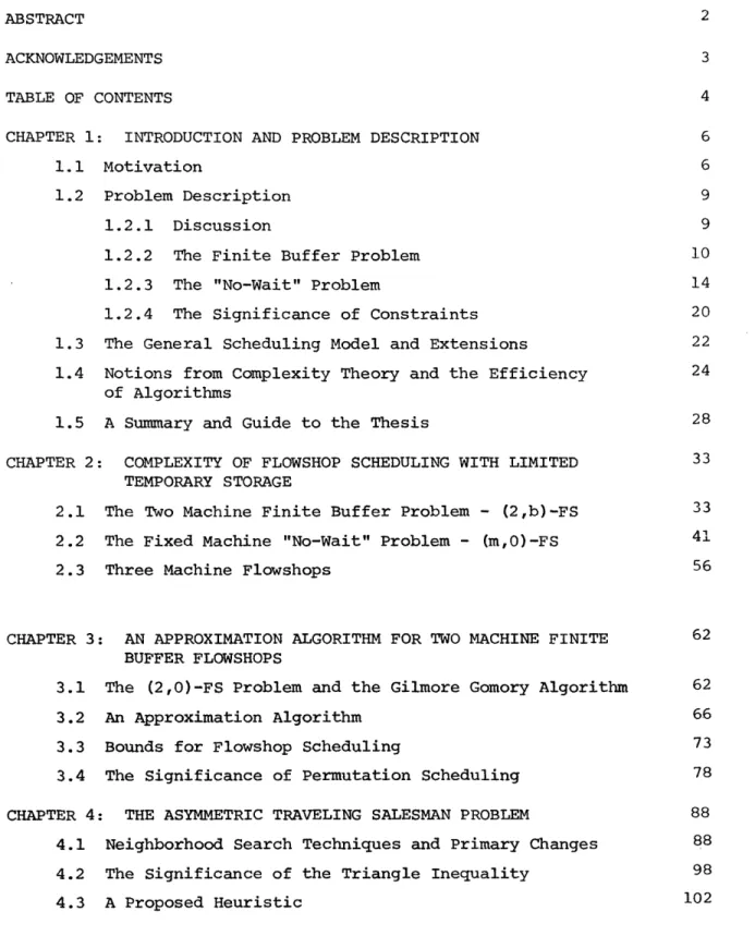
Theorem 2.1.1. The (2,3)-FS problem is NP-complete.

Proof: Suppose that we are given an instance {al,..., a3n

I

of the

3M problem. We construct the following instance of the (2,3)-FS

problem. Consider a set

J

of 4n+2 jobs, with execution times

a) We have n jobs K1,..., K with K. = (2c, c).

ln 1

Also, we have the jobs Ko = (O,c) and K = (c,O).

b) For each i, l<i<3n we have a job Ei = (0, a.).

L is taken to be (2n+l)c.

"4" Suppose a partition exists which has the desired form. That is

each set Ai consists of three elements ag(i,l)' ag(i,2)' a (i 3) such

that for all i, l<i<n j

ag(ij) = c. Then the following schedule

j=1

shown in Figure lla and by its starting times below has length (2n+l)c.

S(KO, 1) = 0 S(K0,2) = 0

S(Ki, i) = 2c(i-1) S(Ki, 2) = 2ci

S(Kn+l, 1) = 2cn

S(K +1, 2) = 2cn + c

S(Eg(il)' 1) = 2c(i-1) S(Eg(i1)' 2) = 2c(i-1)

S(E 1) = 2c(i-1) S(E (i,2)' 2) = 2c(i-1) + ag(il)

S(E 1) = 2c(i-1) S(E g 2) 2c(i-l)+a 1) + ag(i,2)

2

c

K1 K K K

12

n

n+l

K0

I

1

Kn-

K

c c \ E Eg

g(i,l) Eg(i,2) g(i,3)

Figure l]a

c

Eg(i,])' Eg(i,2) ' g(i,3

K Ki

i _-1

"-" Conversely suppose a schedule of length (2n+l)c exists. It is

evident that there is no idle time on either machine. The schedule on

machine 1 has the form K

₀

, , K

K

2 ,

..., K , K

because all K.'s l<i<n

are equivalent. The 3n jobs E. have to be distributed among the n

in-stants 2c(i-1), l<i<n for the first machine. We cannot insert 4 or

more jobs at time 2c(i-1) on machine 1, because since K. has to start

on it no matter which one of the 4 jobs or

Ki_

1

we executed on machine

2 we would violate the buffer constraint, (Figure llb is not permitted).

Therefore, since we have 3n jobs we have to place exactly 3 of them

at each 2c(i-1). Betwee 2c(i-1) and 2ci machine 2 must execute exactly

these 3 jobs and Ki

. 1

The schedule must be saturated thus the three

Ej's

allocated to 2c(i-1) must correspond to three ai's that sum up

to c.

Theorem 2.1.2 The (2,2)-FS problem is NP-complete.

Proof: Suppose we are given an instance {a,..., a3n

I

of the 3M problem.

We construct the following instance of the (2,2)-FS problem.

Consider a set

J

of 4n+2 jobs with execution times (ait,

i) as

follows:

3c

a) We have n jobs K1,..., K with K.

=

(c,

Also, we

1

n

'3c

~7~13c6

have jobs K0 = (0, )and K n+=(, 0).

b) For each l<i<3n we have a job E= (

a).

i 16 I"i 3c

L is taken to be nc + (n+l)

16

"' ' Again if a partition exists we have a schedule as in Figure

12.

K K K1 . -. K_n+l K K 0 ... n E _g(1,1) E E ---g(1,2) g(1,3) 3c 16 Figure 12

Conversely if there is a schedule it must be saturated. On machine

1 between Ki

and K. we cannot have more than three jobs, because the

i-l

1

c

c

buffer would overflow. We now use the property 4 < ai < . We cannot

have more than 3 Ej jobs consecutive, because the processing times on

3c c

machine 2 are -- or at least greater than - . The rest of the argument

16

is as in theorem 2.1.1.

Theorem 2.1.3* The (2.1)-FS problem is NP-complete.

Proof: Suppose that we are given an instance {al,...,a }, {b .b } l''n'''''b2n of the 3MI problem. It is immediately obvious that we can assume that

c/4 < a., b. < c/2, and that the ai, b.'s are multiples of 4n; since

J

1

J

we can always add to the a. and b.'s a sufficiently large integer, and then multiply all integers by 4n. Obviously, this transformation will not affect in any way the existence of a solution for the instance of

the 3MI problem. Consequently, given any such instance of the 3MI problem, we shall construct an instance I of the (2,1)-FS problem such that I

has a schedule with makespan bounded by L iff the instance of 3MI problem were solvable. The instance of the (2,1)-FS problem will have

a set J of 4n+l jobs, with execution times (ai'

3i

)

as follows:

This reduction is due to Prof. Ch.H. Papadimitriou

a) We have n-l jobs K

₁

,..., Kn_

₁

with K. = (c/2,2).

Also

1

we have the jobs Ko = (0,2), and K = (c/2,0).

b) For each 1<i<2n we have a job Bi = (l,bi) and for each

l<i<n we have a job A. = (c/2,a.).

-- 1 1

L is taken to be n(c+2); this complete the construction

of the instance I of the (2,1)-FS.

We shall show that I has a schedule S with 1(S) < L iff the original

instance of the 3MI problem had a solution. First notice that L equals

the sum of all ai's and also of all

.i's; hence p(S) < L iff p(S) = L

and there is no idle time for either machine in S. It follows that K

0

must be scheduled first and K last.

n

We shall need the following lemma:

Lemma If for some j < n, S(K., 2) = k, then there are integers il,

i < 2n such that S(B. , 1) = k, S(B. , 1) = k+l.

2-

I

12

Proof of Lemma.

The lemma says that in any schedule S with no

idle times the first two executions on the first machine of jobs {Bi.}

are always as shown in Figure 13a. Obviously, the case shown in Figure

13b -- the execution of B. on the first machine starts and end in the

middle of another job -- is impossible, because the buffer constraint

is violated in the heavily drawn region. So, assume that we have the

situation in 13c.

However, since all times are multiples of 4n except

for the a's of the Bi's and the 3's of the Kj's, and since no idle time

is allowed in either machine, we conclude that this is impossible.

Similarly, the configuration of Figure 13d is also shown impossible.

Furthermore, identical arguments hold for subsequent executions of Bi

jobs; the lemma follows.

Bi, Bi, Bi

(a)

(b)

Bi

I

I

(c)

(d)

Figure 13

By the lemma, any schedule S of

J

having no idle times must have

a special structure.

It has to start with Ko and then two jobs Bi

Bi are chosen. The next job must have an

a

greater than bi but not

'2 '1

greater than bi + bi ; furthermore it cannot

be a Kj job since these

1 2

jobs must, according to the lemma, exactly precede

two Bi jobs and

then the buffer constraint would be violated.

So we must next execute

an A job and then a Kk job, because of the inequalities c/4 < ai.,

bi < c/2.

Furthermore, we must finish with the Kk job

in the first

machine exactly when we finish the Aj job on

the second, so that we can

schedule two more B jobs (see Figure 14). It follows that any feasible schedule of I will correspond to a decomposition ofthe set B into n

p { ii i

~pairs

{P, ob such that a + C.

I

I

C/2

C/2

1 1

C/2

C/2

2

b, Pi

Pi

bi

bi

j

P

i

2

bi

I

b'

Conversely, if such a partition of B is achievable then we can construct a feasible -- and without idle times -- schedule S by the pattern shown in Figure 14. Hence we have shown that the 3MI problem

reduces to (2,1)-FS, and hence the (2,1)-FS problem is NP-complete.

Let us now notice that the above arguments, for b>l, generalize to show that the (b+2)M problem reduces to the (2. b+l)-FS and that the

(b+2)MI problem reduces to the (2,b)-FS. (e.g., In the (b+2)MI problem we are given a set A of n integers and a set B of (b+l)n integers; the question is whether B can be partitioned into (b+l) tuples P =

b+l

(P ,..., P.

)

such that a. + E p. = c. This problem is easily

i1 1b+l =1

j1

seen to be NP-complete.) Therefore the important conclusion is that Corollary The (2,b)-FS problem is NP-complete for any fixed b, O<b<-.

Let us close this section by commenting on the use of another optimization criterion. If instead of the makespan we wish to examine flowshops under a flowtime criterion we have that the (2,b)-FS is NP--complete for b=y and open for b=O [24]. We conjecture that the (2,1)-FS under a flow time criterion is NP-complete.

2.2 The Fixed Machine "No-Wait" Problem - (m,O)-FS

In certain applications we must schedule flowshops without using any intermediate storage; this is known as the no-wait problem. (For a discussion of this class of problems, see Section 1.2.3).

Theorem 2.2.1* The (4,0)-FS problem is NP-complete

The discussion of this proof follows [31] . This part represents a joint effort with Prof. C.H. Papadimitriou. Personal contributions are the idea to use Hamilton paths in the defined special graphs and the realization of the components of these graphs in terms of 4 machine job systems.

For the purposes of this proof, we introduce next certain special

kinds of directed graphs. Let

J

be an m-machine job system, and let K

be a subset of {1,2,...,m}.

The digraph associated with J with respect

to K,D(J;K) is a directed graph (J,A(J;K)), such that (Ji,J.)

E

A(J;K)

iff job J. can follow job Ji in a schedule S which introduces no idle

I 1

time in the processors in K (e.g., kCK F(i,k) = S(j,k)).

The definition of the set of arcs A(J,K) given above could be made

more formal by listing an explicit set of inequalities and equalities

that must hold among the processing times of the two jobs. To illustrate

this point, we notice that if m=4 and K = {2,3} (Figure 15) the arc

(J,1J2) is included in A(J,K) iff we have

(1) a2 < 81 Y2 > 61 and 82 = Y¥

Machine

II

2

, ..

=....E .

Figure 15

We define

D(m;K)

to be the class of digraphs D such that there

exists a job system J

with D = D(J;K).

We also define the following

class of computational problems, for fixed m > 1 and K C.{1,2,...m}

(m,K)-HAMILTON CIRCUIT PROBLEM

Given an m-machine job system

J,

does D(J;K) have a Hamilton circuit?

We shall prove Theorem 2.2.1 by the following result.

Theorem 2.2.2 The (4;{2,3})-Hamilton circuit problem is NP-complete.

We shall prove Theorem 2.2.2 by employing a general technique for proving Hamilton path problems to be NP-complete first used by Garey, Johnson and Tarjan [16]. (See also [26], [27].) The intuition behind this technique is that the satisfiability problem is reduced to the different Hamilton path problems by creating subgraphs for clauses on one side of the graph and for variables on the other and relating these sebgraphs through "exclusive-or gates" and "or gates" (see Figure 16) We shall introduce the reader to this methodology by the following problem and lemma.

RESTRICTED HAMILTON CIRCUIT PROBLEM

Given a digraph D = (V,A) (with multiple arcs) a set of pairs P of arcs in A and a set of triples T of arcs in A is there a Hamilton circuit C of D such that

a. C traverses exactly one arc from each pair P. b. C traverses at least one arc from each triple T.

LEMMA 1. The restricted Hamilton circuit problem is NP-complete.

Proof. We shall reduce 3-satisfiability to it. Given a formula F in-voling n variables xl,...,x and having m clauses C1,...,C with 3 literals each, we shall construct a digraph D (with possibly multiple arcs), a set of pairs P (two arcs in a pair are denoted as in Figure 17a) and a set of triples T (Figure 17b), such that D has a feasible --with respect to P and T -- Hamilton circuit iff the formula is satis-fiable.

The construction is a rather straight-forward "compilation." For each variable x.j we have five nodes aj, bj, cj, d. and ej, two copies of each of the arcs (a.,bj) and (dj,ej) and one copy of each of the arcs

(bj,cj ) and (c.,d.) (see Figure 16): The "left" copies of (aj,bj) and (dj,ej) form a pair P. We also connect these sub-digraphs in series via the new nodes f.. For each clause C. we have the four nodes

3~~~ 1

u., v., w. and z. and two copies of each of the arcs (u.,v.) (v.,w.)

1 1 1 1 1 . 1 1

and (w.,zi). Again the "left" copies of these three arcs form a triple in T. These components are again linked in series via some

other nodes called Yi (see Figure 16). Also we have the arcs (Ym+lfl) and (f lYl). To take into account the structure of the formula, we connect in a pair P the right copy of (ui,vi) with the left copy of

(a.,b.) if the first literal of C. is x., and to the left copy of (d.,ej) if it is x.; we repeat this with all clauses and literals. An illustration is shown in Figure 16.

It is not hard to show that D has a feasible Hamilton circuit if and only if F is satisfiable. Any Hamilton circuit C of D must -have

a special structure: it must traverse the arc (y +1 fl)

,

and then the arcs of the components corresponding to variables. Because of the

pairs P, if C traverses the left copy of (ai,bi), it has to traverse the right copy of (di,e.i); we take this to mean that xi is true otherwise if the right copy of (ai,bi) and the left of (d.,ei) are traversed, Xi is false. Then C traverses the arc (fm+lY _l) and the components corresponding to the clauses, one by one. However, the left copies of arcs corresponding to literals are traversed only in the case that the corresponding literal is true; thus, the restrictions due to the triples T are satisfied only if all the clauses are satisfied by the truth assignment mentioned above. (In Figure 16, x1 = false, x2 - false, X3 = true.)

Conversely using any truth assignment that satisfies F, we can construct, as above, a feasible Hamilton circuit for D. This proves the lemma. o

What this lemma (in fact, its proof) essentially says is that for a Hamilton circuit problem to be NP-complete for some class of digraphs, it suffices to show that one can construct special purpose digraphs in this class, which can be used to enforce implicitly the constraints imposed by P (an exclusive-or constraint) and T (an or constraint). For example, in order to show that the unrestricted Hamilton circuit problem is NP-complete, we just have to persuade ourselves that the

digraphs shown in Figure 17a and b can be used in the proof of Lemma 1 instead of the P and T connectives, respectively [27]. Garey, Johnson and Tarjan applied this technique to planar, cubic, triconnected graphs

W22

e.-2

~u

2

fb2

3

--

e-e

f4

(x v

X2

V

X

₃

) A

(X

V XV

X3)

Figure

16

UI

I

,~~~~~~~~~~~~~~~~~~~~~~~~~~~

Yt'-~1-

_wt

_{2V 3hXV}

₂

₃

,--,-~_~rc2

f

Figure

16~~~~~~~!f

VV

V

_U

Ui,

--

:U'

l

...

(a)

In Figure 17a the Hamilton circuit either passes through u and u'

or through v and v'.

In Figure 17b no Hamilton circuit can contain all

the arcs (u,v), (v,w) and (w,z).

Our proof of Theorem 2.2.2 follows the same lines.

There are

how-ever, several complications due to the restricted nature of the digraphs

that concern us here.

First, we have to start with a special case of

the satisfiability problem.

LEMMA 2. The 3-satisfiability problem remains NP-complete even if each

variable is restricted to appear in the formula once or twice unnegated

and once negated.

Proof. Given any formula we first modify it so that each variable appears

at most three times.

Let x be a variable appearing k > 3 times in the

formula. We replace the first occurrence of x by (the new variable)

xl, the second with x

2

, etc. We then add the clauses (xl v x

2)

v

x

3)...(xk v

x

-- which are, of course xi=

x2= x

3

... x

k

in

conjuctive normal form. We then omit any clause that contains a literal,

which appears in the formula either uniformly negated or uniformly

un-negated. Finally if x is a variable appearing twice negated, we

sub-stitute y for x in the formula, where y is a new variable. The

re-sulting formula is the equivalent of the orignal under the restrictions

of Lemma 2. o

Secondly, realizing special-purpose digraphs in terms of job systems

presents us with certain problems. Although our special-purpose digraphs

will be similar to those in Figure 17, certain modifications cannot be

avoided. A digraph in D(4;{2,3}) must be realizable in terms of some