HAL Id: hal-00657340
https://hal-upec-upem.archives-ouvertes.fr/hal-00657340
Submitted on 16 Mar 2012
HAL is a multi-disciplinary open access archive for the deposit and dissemination of sci-entific research documents, whether they are pub-lished or not. The documents may come from teaching and research institutions in France or abroad, or from public or private research centers.
L’archive ouverte pluridisciplinaire HAL, est destinée au dépôt et à la diffusion de documents scientifiques de niveau recherche, publiés ou non, émanant des établissements d’enseignement et de recherche français ou étrangers, des laboratoires publics ou privés.
A faster algorithm for finding minimum Tucker
submatrices
Guillaume Blin, Romeo Rizzi, Stéphane Vialette
To cite this version:
Guillaume Blin, Romeo Rizzi, Stéphane Vialette. A faster algorithm for finding minimum Tucker sub-matrices. Theory of Computing Systems, Springer Verlag, 2012, 51 (3), pp.270-281. �10.1007/s00224-012-9388-1�. �hal-00657340�
A faster algorithm for finding
minimum Tucker submatrices
Guillaume Blin1, Romeo Rizzi2, and St´ephane Vialette1
1
Universit´e Paris-Est, LIGM - UMR CNRS 8049, France. {gblin,vialette}@univ-mlv.fr
2
Dipartimento di Matematica ed Informatica (DIMI) Universit degli Studi di Udine, Italy. [email protected]
Abstract. A binary matrix has the Consecutive Ones Property (C1P) if its columns can be ordered in such a way that all 1s on each row are consecutive. Algorithmic issues of the C1P are central in computa-tional molecular biology, in particular for physical mapping and ances-tral genome reconstruction. In 1972, Tucker gave a characterization of matrices that have the C1P by a set of forbidden submatrices, and a sub-stantial amount of research has been devoted to the problem of efficiently finding such a minimum size forbidden submatrix. This paper presents a new O(∆3m2(m∆ + n3)) time algorithm for this particular task for a m×n binary matrix with at most ∆ 1-entries per row, thereby improving the O(∆3m2(mn + n3)) time algorithm of [M. Dom, J. Guo and R. Nie-dermeier, Approximation and fixed-parameter algorithms for consecutive ones submatrix problems, Journal of Computer and System Sciences, 76(3-4): 204-221, 2010 ]. Moreover, this approach can be used – with a much heavier machinery – to address harder problems related to Minimal Conflicting Set [G. Blin, R. Rizzi, and S. Vialette. A Polynomial-Time Algorithm for Finding Minimal Conflicting Sets, Proc. 6th International Computer Science Symposium in Russia (CSR), 2011 ].
1 Introduction
A binary matrix has the Consecutive Ones Property (C1P) if its columns can be ordered in such a way that all 1s on each row are consecutive. Both deciding if a given binary matrix has the C1P and finding the cor-responding columns permutation can be done in linear time [9, 17, 18, 22–24, 27, 30]. The C1P of matrices has a long history and it plays an important role in combinatorial optimization, including application fields such as scheduling [6, 20, 21, 35], information retrieval [25], and railway optimization [28, 29, 32] (see [15] for a recent survey). Furthermore, algo-rithmic aspects of the C1P turn out to be of particular importance for physical mapping [2, 12, 26] and ancestral genome reconstruction [1, 11]. (see also [10, 3–5, 13, 31] for other applications in computational molecular
biology). Actually, our main motivation for studying algorithmic aspects of the C1P comes from minimal conflicting sets in binary matrices in the context of ancestral genome reconstruction [?]. A minimal conflicting set of rows in a binary matrix is a set of rows R that does not have the C1P but such that any proper subset of R has the C1P (a similar definition applies for columns). Tucker [34] has characterized the binary matrices that have the C1P by a set of forbidden submatrices, and the aim of this paper is to lay the foundations for efficiently computing minimal conflict-ing sets by presentconflict-ing a new efficient algorithm for findconflict-ing such minimum size forbidden Tucker submatrices [8].
Recently, Dom et al. [16] investigated some natural problems aris-ing when a matrix M does not have the C1P property (the C1P is in-deed a desirable property than often leads to efficient algorithms): find a minimum-cardinality set of columns to delete such that the resulting matrix has the C1P, find a minimum-cardinality set of rows to delete such that the resulting matrix has the C1P, and find a minimum-cardinality set of 1-entries in the matrix that shall be flipped (that is, replaced by 0-entries) such that the resulting matrix has the C1P. All these problems are NP-hard even for simple instances [19, 33], and hence Dom et al. have focused on approximation and parameterized complexity issues. To this end, they have provided a technical solution based on efficiently detecting forbidden Tucker submatrices [34].
In this paper, we presents a new O(∆3m2(m∆ + n3)) time algorithm for finding a a minimum size forbidden Tucker submatrix in m × n bi-nary matrices with at most ∆ 1-entries per row, thereby improving the O(∆3m2(mn + n3)) time algorithm of Dom et al. [16, 15].
This paper is organized as follows: we first recall basic definitions in Section 2, and we then formally introduce the considered problem. In Section 3, we briefly recall the algorithm of Dom et a. Section 4 is devoted to presenting out technical improvement and we consider in Section 5 matrices with unbounded ∆.
2 Preliminaries
All graphs are considered as undirected. Given a graph G = (V, E), let N (v) = {u|(u, v) ∈ E} denote the neighborhood of vertex v in G. The neighborhood described above does not include v itself, and is more specif-ically the open neighborhood of v; it is also possible to define a neigh-borhood in which v itself is included, called the closed neighneigh-borhood. For any subset V0 ⊆ V of vertices, let G[V0] denote the subgraph of G
in-duced by the vertices of V0 (i.e., G0 = (V0, {(u, v) ∈ E|u, v ∈ V0})). An induced cycle is a cycle that is an induced subgraph of G; induced cycles are also called chordless cycles. An asteroidal triple is an independent set of three vertices such that each pair is joined by a path that avoids the neighborhood of the third.
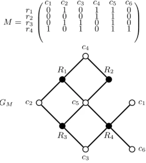
A binary matrix has the Consecutive Ones Property (C1P) if its columns can be ordered in such a way that all 1s on each rows are con-secutive. For a matrix M , we let ri and cj stand for the ith row and
the jth column of M , respectively. Let M be a m × n binary matrix. Its corresponding bipartite graph G(M ) = (VM, EM) is defined as follows:
VM = R ∪ C, where R = {ri : 1 ≤ i ≤ m} is the set of rows of M
and C = {ci : 1 ≤ i ≤ n} is the set of columns of M , and two vertices
ri ∈ R and cj ∈ C are connected by an edge if and only if M [i, j] = 1.
Equivalently, M is the reduced adjacency matrix of G(M ) (i.e. the non-redundant portion of the full adjacency matrix for the bipartite graph). Actually, it will be convenient to define G(M ) as a vertex-colored bipartite graph: each ri ∈ R (row vertex) is colored black and each cj ∈ c (column
vertex) is colored white. See Figure 1 for an illustration (we use capital letters for black vertices and uncapitalized letters for white vertices).
M = c1 c2 c3 c4 c5 c6 r1 0 1 0 1 1 0 r2 0 0 0 1 1 0 r3 0 1 1 0 1 0 r4 1 0 1 0 1 1 c2 GM R1 R3 c4 c5 c3 R2 R4 c1 c6
Fig. 1. A binary matrix and its corresponding vertex-colored bipartite graph.
The following result of Tucker links the C1P for binary matrices to asteroidal triples.
Theorem 1 ([34], Theorem 6). A binary matrix has the C1P if and only if its corresponding vertex-colored bipartite graph does not contain a white asteroidal triple, i.e. an asteroidal triple on column vertices.
Moreover, Tucker has characterized the binary matrices that have the C1P by a set of forbidden submatrices (the number of vertices in the forbidden graph defines the size of the Tucker configuration).
Theorem 2 ([34], Theorem 9). A binary matrix has the C1P if and only if it contains none of the matrices MIk, MIIk, MIIIk (k ≥ 1), MIV
and MV depicted in Figure 2.
Fig. 2. Forbidden Tucker submatrices represented as vertex-colored bipartite graphs [34]. Black and white vertices correspond to rows and columns, respectively.
3 The algorithm of Dom et al.
In [16], Dom et al. provided an algorithm for finding a forbidden Tucker submatrix (i.e., one of T = {MIk, MIIk, MIIIk, MIV, MV}) in a given
binary matrix. The general algorithm is as follows. For each white as-teroidal triple u, v, w of G(M ), compute the sum of the lengths of three shortest paths connecting two by two u, v and w (each path has to avoid the closed neighborhood of the third vertex). Select an asteroidal triple u, v, w of G(M ) with minimum total length of the paths connecting each
Time complexity
Tucker configuration Dom et al. Our contribution MIk and MIIk O(∆mn 2 + n3) O(∆3m2(n + ∆m)) MIIIk O(∆ 3 m3n + ∆2m2n2) O(∆mn2(n + ∆m))
MIV O(∆3m2n3) Algorithm of Dom et al. used verbatim
MV O(∆4m2n) Algorithm of Dom et al. used verbatim
Overall O(∆3m2(mn + n3)) O(∆3m2(∆m + n3))
Table 1. Comparing our results with Dom et al. [16, 15].
pair of vertices and return the rows and columns of M that correspond to the vertices that occur along the three shortest paths. The authors proved that the returned submatrix does contain a forbidden Tucker sub-matrix of T but which is not necessarily of minimum size (for MIIIk, MIV
and MV). Indeed, since the three shortest paths may share some vertices,
the sum of the lengths of the three paths is not necessarily the number of vertices in the union of the three paths. However, Dom et al. showed that the returned submatrix contains at most three extra columns (resp. five extra rows) compared with a forbidden Tucker submatrix with min-imum number of columns (resp. rows). To overcome this problem, they provided another algorithm devoted to MIIIk, MIV and MV submatrices.
More precisely, they used the similarity between MIIIk and MIk to reduce
the problem to a minimum-size chordless cycle search. For MIV and MV,
they provided an exhaustive search. On the whole, Dom et al. provided an algorithm for finding a forbidden Tucker submatrix in a given matrix M (assuming M does not have the C1P) in O(∆3m2n(m + n2)) time, where m is the number of rows of M , n is the number of columns of n, and ∆ is the maximum number of 1-entries in a row. More precisely, the authors provided a O(∆mn2+ n3) time algorithm for finding a MIk
or MIIk submatrix, a O(∆3m3n + ∆2m2n2) time algorithm for finding a
MIIIk submatrix, a O(∆3m2n3) time algorithm for finding a MIV
sub-matrix, and a O(∆4m2n) time algorithm for finding a MV submatrix. See
Table 1.
The main contribution of this paper is a simple O(∆3m2 (m∆ + n3)) time algorithm for finding a minimum size forbidden Tucker submatrix. Our technical improvement on Dom et al. [16, 15] is based on shortest paths and two graph pruning techniques: clean and complement clean (to be defined in the next section). Graph pruning techniques were in-troduced by Conforti and Rao [14]. One has to note that graph pruning technique does not always succeed in the detection of induced configu-rations. Indeed, in [7] Bienstock gave negative results among which one
can find an NP-completeness proof for the problem of deciding whether a graph contains an odd chordless cycle containing a given vertex. This negative result, which in attacking the perfect graph conjecture was use-ful in posing limits in what could have been a reasonable approach, also demonstrates that not everything can be done with the detection of in-duced configurations.
4 Fast detection of minimum size forbidden Tucker submatrices
In this section, we design a general algorithm that reports in polynomial-time the smallest Tucker configuration of a given matrix M if it exists. To do so, we seek for any subgraph of G(M ) that corresponds to a submatrix of T .
Let us introduce the clean and cpl clean cleaning operations. Let M be a binary matrix and G(M ) = (VM, EM) be the corresponding
vertex-colored bipartite graph. Let v be a vertex of G(M ), then cleanG(M )(v)
is the graph obtained by removing from G(M ) all neighbors of v, i.e., G(M )[VM \ N (v)]. Let v be a vertex of G(M ), then cpl cleanG(M )(v)
(read complement clean)) is the graph obtained by removing from G(M ) all vertices that do not belong to the same partition nor the neighborhood of v, i.e., G(M )[N (v) ∪ {u : color(u) = color(v)}]. For the sake of simplicity, we shall write cleanG(M )(u1, u2, . . . , uk) for the sequence
G1 ← cleanG(M )(u1), G2 ← cleanG1(u2), .. . Gk ← cleanGk−1(uk), Return Gk,
and cpl cleanG(M )(u1, u2, . . . , uk) for the sequence
G1 ← cpl cleanG(M )(u1),
G2 ← cpl cleanG1(u2),
. . . ,
Gk ← cpl cleanGk−1(uk),
We now focus on the bipartite graphs that represent Tucker con-figurations (see Figure 2) and define our guessing functions. Define the function guessI(G(M )) (reps. guessII(G(M ))) that returns all possible sets of vertices {x, y, z, A, B} ⊆ VM as defined for the Tucker
config-uration MIk (resp. MIIk) in Figure 2. Furthermore, Define the function
guessIII(G(M )) that returns all possible sets of vertices {x, y, z, A} ⊆ VM
as defined for the Tucker configuration MIIIk in Figure 2. Of particular
importance, in the presented algorithms, guessed vertices will never be affected (i.e., deleted) by the clean and cpl clean functions.
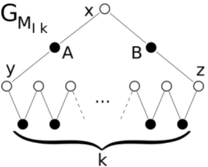
Fig. 3. MIk Tucker configuration.
Lemma 1. Let M be m × n binary matrix with at most ∆ 1-entries per row. Algorithm 1 computes the smallest submatrix G(MIk) in G(M ) in
O(m2∆3(n + ∆m)) time (if such a submatrix exists).
Proof. We apply Algorithm 1 to G(M ). Let us first prove that if G(MIk)
occurs in G(M ), then Algorithm 1 finds it. Suppose G0 = G(MIk) occurs
in G(M ). Then among all the guessed 5-plets x, y, z, A, B (Line 1), there should be at least one guess such that x, y, z, A, B are part of the vertices of G0. By definition, G0 is a chordless cycle. Therefore, clean(x, A, B) preserves G0 since in G0, (1) x is only connected to vertices A and B, (2) A is only connected to vertices x and y, and (3) B is only connected to x and z. Therefore, looking for a shortest path p in the pruned graph between y and z after having removed A and B ensures the minimality of the returned solution.
The guessing can be done in O(m2∆3) time. Indeed, once A has been identified, one can (i) select x and y among the at most ∆ neighbors of A, and (ii) identify B and one of its at most ∆ neighbors as z such that x ∈ N (B) and z /∈ {x, y}. For each such guessing, the cleaning of x, A, B
Algorithm 1 Finding G(MIk) in G(M )
1: for all {x, y, z, A, B} ← guessI(G(M )) do 2: G1← cleanG(M )(x,A,B)
3: Remove the vertices A and B from G1. In the resulting graph, find a shortest
path p from y to z 4: if p exists then
5: S ← {x, y, z, A, B} ∪ {u : u ∈ p} 6: return the induced subgraph G(M )[S] 7: end if
8: end for 9: return None
can be done in O(∆ + m) time. Finally, a shortest path between y and z can be computed in O(n+∆m) time (the pruned graph has at most m+n vertices and ∆m edges). On the whole, Algorithm 1 is O(m2∆3(n + ∆m))
time. ut
Fig. 4. MIIkTucker configuration.
Lemma 2. Let M be a m × n binary matrix with at most ∆ 1-entries per row. Algorithm 2 computes the smallest submatrix G(MIIk) in G(M )
in O(m2∆3(n + ∆m)) time (if such a submatrix exists).
Proof. We apply Algorithm 2 to G(M ). Let us first prove that if G(MIIk)
occurs in G(M ), then Algorithm 2 finds it. Suppose G0 = G(MIIk) occurs
in G(M ). Then among all the guessed 5-plets x, y, z, A, B in Line 1, there must be at least one guess such that x, y, z, A, B are part of the vertices of G0. By definition, in G0 any unguessed white node is in the neighborhood of both A and B. Thus, cpl clean(A, B) preserves G0 since (1) y (the only white node not in the neighborhood of B) has been guessed, and (2)
z (the only white node not in the neighborhood of A) has been guessed. Moreover, in G0 x should be only connected to A and B. Thus, clean(x) preserves G0. Finally, looking for a shortest path p in the pruned graph between y and z after having removed A and B ensures the minimality of the returned solution.
Algorithm 2 Finding G(MIIk) in G(M )
1: for all {x, y, z, A, B} ← guessII(G(M )) do
2: G1← cpl cleanG(M )(A, B)
3: G2← cleanG1(x)
4: Remove the vertices A and B from G2. In the resulting graph, find a shortest
path p from y to z 5: if p exists then
6: S ← {x, y, z, A, B} ∪ {u : u ∈ p} 7: return the induced subgraph G(M )[S] 8: end if
9: end for 10: return None
The guessing can be done in O(m2∆3) time. For each guessing, the
cleaning/complement-cleaning of x, A, and B can be done in O(n + m) time. Finally, a shortest path between y and z can be computed in O(n + ∆m) time (the pruned graph has at most ∆ + n vertices and ∆m edges). On the whole, Algorithm 2 is O(m2∆3(n + ∆m)) time. ut
Fig. 5. MIIIk Tucker configuration.
Lemma 3. Let M be a m × n binary matrix with at most ∆ 1-entries in each row. Algorithm 3 computes the smallest G(MIIIk) in G(M ) in
Algorithm 3 Finding G(MIIIk) in G(M )
Proof. 1: for all {x, y, z, A} ← guessIII(G(M )) do 2: G1← cpl cleanG(M )(A)
3: G2← cleanG1(x)
4: Remove the vertex A from G2. In the resulting graph, find a shortest path p
from y to z. 5: if p exists then
6: S ← {x, y, z, A} ∪ {u : u ∈ p}
7: return the induced subgraph G(M )[S] 8: end if
9: end for 10: return None
We apply Algorithm 3 to G(M ). Let us first prove that if G(MIIIk)
occurs in G(M ), then Algorithm 3 finds it. Suppose G0 = G(MIIIk) occurs
in G(M ). Then among all the guessed 4-plets x, y, z, A in Line 1, there must be at least one guess such that x, y, z, A are part of the vertices of G0. By definition, in G0 any unguessed white node is in the neighborhood of A. Thus, cpl clean(A) preserves G0 since in G0 y and z (the only white nodes not in the neighborhood of A) have been guessed. Moreover, in G0 x is only connected to A. Therefore, clean(x) preserves G0. Finally, looking for a shortest path p in the pruned graph between y and z after having removed A ensures the minimality of the returned solution.
The guessing can be done in O(m∆n2) time. Indeed, once A has been identified, one can (i) select x among the at most ∆ neighbors of A and (ii) then identify y and z. For each such guessing, the cleaning/complement-cleaning of x and A can be done in O(n+m) time. Finally, a shortest path between y and z can be computed in O(n + ∆m) time (the pruned graph has at most ∆ + n vertices and ∆m edges). On the whole, Algorithm 3
is O(m∆n2(n + ∆m)) time. ut
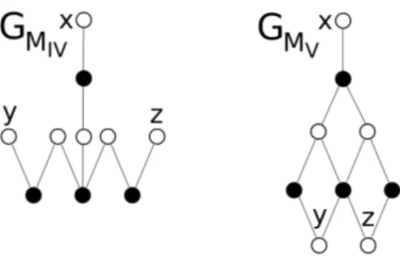
As for G(MIV) and G(MV), a simple brute-force search yields the
time complexity detailed in Lemma 4.
Lemma 4 ([16], Proposition 5.3). Let M be a m × n binary matrix with at most ∆ 1-entries per row. The smallest G(MIV) (resp. G(MV))
in G(M ) can be computed in O(∆3m2n3) (resp. O(∆4m2n) time) if it
exists.
We are now ready to state the main result of this paper (Table 1 compares our results with Dom et al. [16].).
Fig. 6. MIV and MV Tucker configurations.
Theorem 3. Let M be a m × n binary matrix that does not have the C1P with at most ∆ 1-entries per row. A minimum size forbidden Tucker submatrix that occurs in M can be found in O(∆3m2(∆m + n3)) time.
Notice that our results do not improve on the ones of Dom et al. [16] for large ∆. Furthermore, our results also do not improve on the ones of Dom et al. [16] for each Tucker configuration. For example, if m = n, our algorithm has time complexity O(∆4m3) for MIk and MIIkTucker
config-urations, whereas Dom et al.’s algorithm has time complexity O(∆ m3).
5 Matrices with unbounded ∆
As mentioned in [16], a natural question is concerned with the complex-ity of the problem when the number of 1s per row is unbounded. One can distinguish two subcases: the maximum number of 1s per column is bounded (say by C) or not. In the following, we prove that using a sim-ilar approach to the one used in the preceding section, one can achieve an O(C2n3(m + C2n)) (resp. O(n4m4)) time complexity for the bounded (resp. unbounded) case.
Theorem 4. Let M be a m × n binary matrix with at most C 1-entries per column. A minimum size forbidden Tucker submatrix that occurs in M can be found in O(C2n3(m + C2n)) time.
Proof. We apply Algorithms 1, Algorithms 2, and Algorithms 3 to find any forbidden submatrix of type MIk, MIIk or MIIIk. Let us now analyze
the time complexity.
For Algorithm 1, the guessing can be done in O(n3C2) time. Indeed, once x has been identified, one can select A and B among the at most C
neighbors of x and then identify y and z such that y ∈ N (A), y 6∈ N (B), z ∈ N (B), z 6∈ N (A) and x 6= y 6= z. For each such guessing, the cleaning of x, A, and B can be done in O(C + n) time. Finally, a shortest path between y and z can be computed in O(m + Cn) time (the pruned graph has at most m + n vertices and Cn edges). We conclude that Algorithm 1 is O(C2n3(m + Cn)) time.
For Algorithm 2, the guessing can also be done in O(n3C2). For each such guessing, the cleaning/complement-cleaning of x, A and B can be done in O(C + n) time. Finally, a shortest path between y and z can be computed in O(m + Cn) time (the pruned graphs has at most m + n vertices and Cn edges). We conclude that Algorithm 2 is O(C2n3(m +
Cn)) time.
As for Algorithm 3, the guessing can be done in O(n3C) time. Indeed, once x has been identified, one can select A among the at most C neigh-bors of x and then identify y and z such that y 6∈ N (A), z 6∈ N (A) and x 6= y 6= z. For each such guessing, the cleaning/complement-cleaning of x and A can be done in O(C + n) time. Finally, a shortest path between y and z can be computed in O(m + Cn) time (the pruned graph has at most m + n vertices and Cn edges). We conclude that Algorithm 3 is O(Cn3(m + Cn)) time.
MIV and MV forbidden submatrices deserve careful consideration.
Indeed, a direct application of Proposition 5.3 [16] for finding MIV and
MV forbidden submatrices results in a O(n6) time algorithm. We use the
following strategy: (i) Select the central three white nodes u, v, and w (distinct from x, y and z) among the O(n3) such triples, (ii) select four black nodes that are neighbors of at least one of u, v, or w among the O(C4) such 4-plets, and (iii) for each such combination check in O(n)
time whether every columns of the matrix MIV appears at least once in
the submatrix induced by the selected rows.
A submatrix of the type MV can be found analogously: (i) select the
two central white nodes (distinct from x, y, and z) among the O(n2) such triples, (ii) select four black nodes that are neighbors of at least one of u and v among the O(C4) such 4-plets, and (iii) for each such combination check in O(n) time whether every columns of the matrix MV appears at
least once in the submatrix induced by the selected rows. ut Replacing C by m in the above yields the following result.
Theorem 5. Let M be m × n binary matrix. A minimum size forbidden Tucker submatrix that occurs in M can be found in O(n4m4) time.
References
1. Z. Adam, M. Turmel, C. Lemieux, and D. Sankoff. Common intervals and symmet-ric difference in a model-free phylogenomics, with an application to streptophyte evolution. J. Comput. Biol., 14:436–445, 2007.
2. F. Alizadeh, R. Karp, D. Weisser, and G. Zweig. Physical mapping of chromosomes using unique probes. J. Comput. Biol., 2:159–184, 1995.
3. E. Althaus, S. Canzar, M.R. Emmett, A. Karrenbauer, A.G. Marshall, A. Meyer-Baese, and H. Zhang. Computing h/d-exchange speeds of single residues from data of peptic fragments. In ACM Press, editor, 23rd ACM Symposium on Applied Computing SAC ’08, page 12731277, 2008.
4. J.E. Atkins, E.G. Boman, and B. Hendrickson. A spectral algorithm for seriation and the consecutive ones problem. SIAM J. Comput., 28(1):297310, 1998. 5. J.E. Atkins and M. Middendorf. On physical mapping and the consecutive ones
property for sparse matrices. Discrete Appl. Math., 71(13):2340, 1996.
6. J. J. Bartholdi, J. B. Orlin, and H. D. Ratliff. Cyclic scheduling via integer pro-grams with circular ones. Oper Res, 28(5):1074–1085, 1980.
7. Dan Bienstock. On the complexity of testing for odd holes and induced odd paths. Discrete Math., 90(1):85–92, 1991.
8. G. Blin, R. Rizzi, and S. Vialette. General framework for minimal conflicting set. Technical report, Universit´e Paris Est, I.G.M., jan 2010.
9. K.S. Booth and G.S. Lueker. Testing for the consecutive ones property, interval graphs, and graph planarity using pq-tree algorithms. J. Comput. System Sci., 13:335379, 1976.
10. C. Chauve, J. Manˇuch, and M. Patterson. On the gapped consecutive ones prop-erty. In Proc. 5th European conference on Combinatorics, Graph Theory and Appli-cations (EuroComb), Bordeaux, France, volume 34 of Electronic Notes on Discrete Mathematics, pages 121–125, 2009.
11. C. Chauve and ´E. Tannier. A methodological framework for the reconstruction of contiguous regions of ancestral genomes and its application to mammalian genome. PLoS Comput. Biol., 4:paper e1000234, 2008.
12. T. Christof, M. J¨unger, J. Kececioglu, P. Mutzel, and G. Reinelt. A branch-and-cut approach to physical mapping of chromosome by unique end-probes. J. Comput. Biol., 4:433–447, 1997.
13. T. Christof, M. Oswald, and G. Reinelt. Consecutive ones and a betweenness prob-lem in computational biology. In Springer, editor, 6th International Conference on Integer Programming and Combinatorial Optimization IPCO ’98, volume 1412 of Lecture Notes in Comput. Sci., page 213228, 1998.
14. Michele Conforti and M. R. Rao. Structural properties and decomposition of linear balanced matrices. Mathematical Programming, 55:129–168, 1992.
15. M. Dom. Algorithmic aspects of the consecutive-ones property. Bull. Eur. Assoc. Theor. Comput. Sci. EATCS, 98:2759, 2009.
16. M. Dom, J. Guo, and R. Niedermeier. Approximation and fixed-parameter algo-rithms for consecutive ones submatrix problems. Journal of Computer and System Sciences, 76(3-4), 2010.
17. D.R. Fulkerson and O.A. Gross. Incidence matrices and interval graphs. Pacific J. Math., 15(3):835855, 1965.
18. M. Habib, R.M. McConnell, C. Paul, and L. Viennot. Lex-bfs and partition refine-ment, with applications to transitive orientation, interval graph recognition and consecutive ones testing. Theoret. Comput. Sci., 234(12):5984, 2000.
19. M. Hajiaghayi and Y. Ganjali. A note on the consecutive ones submatrix problem. Information Processing Letters, 83(3):163166, 2002.
20. Refael Hassin and Nimrod Megiddo. Approximation algorithms for hitting objects with straight lines. Discrete Applied Mathematics, 30(1):29 – 42, 1991.
21. Dorit S. Hochbaum and Asaf Levin. Cyclical scheduling and multi-shift scheduling: Complexity and approximation algorithms. Discrete Optimization, 3(4):327 – 340, 2006.
22. W.-L. Hsu. A simple test for the consecutive ones property. J. Algorithms, 43(1):116, 2002.
23. W.-L. Hsu and R.M. McConnell. Pc trees and circular-ones arrangements. Theoret. Comput. Sci., 296(1):99116, 2003.
24. N. Korte and R.H. Mhring. An incremental linear-time algorithm for recognizing interval graphs. SIAM J. Comput., 18(1):6881, 1989.
25. Lawrence T. Kou. Polynomial complete consecutive information retrieval prob-lems. SIAM J. Comput., 6(1):67–75, 1977.
26. W.-F. Lu and W.-L. Hsu. A test for the consecutive ones property on noisy data – application to physical mapping and sequence assembly. J. Comput. Biol., 10:709– 735, 2003.
27. R.M. McConnell. A certifying algorithm for the consecutive-ones property. In ACM Press, editor, 15th Annual ACMSIAM Symposium on Discrete Algorithms SODA ’04, page 768777, 2004.
28. S. Mecke, A. Schbel, and D. Wagner. Station location complexity and approxi-mation. In 5th Workshop on Algorithmic Methods and Models for Optimization of Railways ATMOS ’05, Dagstuhl, Germany, 2005.
29. S. Mecke and D. Wagner. Solving geometric covering problems by data reduction. In Springer, editor, 12th Annual European Symposium on Algorithms ESA ’04, volume 3221 of Lecture Notes in Comput. Sci., page 760771, 2004.
30. J. Meidanis, O. Porto, and G.P. Telles. On the consecutive ones property. Discrete Appl. Math., 88:325354, 1998.
31. M. Oswald and G. Reinelt. The simultaneous consecutive ones problem. Theoret. Comput. Sci., 410(2123):19861992, 2009.
32. Nikolaus Ruf and Anita Schbel. Set covering with almost consecutive ones property. Discrete Optimization, 1(2):215 – 228, 2004.
33. J. Tan and L. Zhang. The consecutive ones submatrix problem for sparse matrices. Algorithmica, 48(3):287299, 2007.
34. A.C. Tucker. A structure theorem for the consecutive 1s property. Journal of Combinatorial Theory. Series B, 12:153162, 1972.
35. A.F. Veinott and H.M. Wagner. Optimal capacity scheduling. Oper Res, 10:518– 547, 1962.
![Fig. 2. Forbidden Tucker submatrices represented as vertex-colored bipartite graphs [34]](https://thumb-eu.123doks.com/thumbv2/123doknet/14430243.515032/5.892.288.634.428.710/forbidden-tucker-submatrices-represented-vertex-colored-bipartite-graphs.webp)
![Table 1. Comparing our results with Dom et al. [16, 15].](https://thumb-eu.123doks.com/thumbv2/123doknet/14430243.515032/6.892.202.721.191.304/table-comparing-results-dom-et-al.webp)