HAL Id: hal-01322207
https://hal.inria.fr/hal-01322207
Submitted on 26 May 2016
HAL is a multi-disciplinary open access
archive for the deposit and dissemination of sci-entific research documents, whether they are pub-lished or not. The documents may come from teaching and research institutions in France or abroad, or from public or private research centers.
L’archive ouverte pluridisciplinaire HAL, est destinée au dépôt et à la diffusion de documents scientifiques de niveau recherche, publiés ou non, émanant des établissements d’enseignement et de recherche français ou étrangers, des laboratoires publics ou privés.
Kamyar Azizzadenesheli, Alessandro Lazaric, Animashree Anandkumar
To cite this version:
Kamyar Azizzadenesheli, Alessandro Lazaric, Animashree Anandkumar. Reinforcement Learning of POMDPs using Spectral Methods. Proceedings of the 29th Annual Conference on Learning Theory (COLT2016), Jun 2016, New York City, United States. �hal-01322207�
Reinforcement Learning of POMDPs using Spectral Methods
Kamyar Azizzadenesheli∗ KAZIZZAD@UCI.EDU
University of California, Irvine
Alessandro Lazaric† ALESSANDRO.LAZARIC@INRIA.FR
Institut National de Recherche en Informatique et en Automatique, (Inria)
Animashree Anandkumar‡ A.ANANDKUMAR@UCI.EDU
University of California, Irvine
Abstract
We propose a new reinforcement learning algorithm for partially observable Markov decision pro-cesses (POMDP) based on spectral decomposition methods. While spectral methods have been previously employed for consistent learning of (passive) latent variable models such as hidden Markov models, POMDPs are more challenging since the learner interacts with the environment and possibly changes the future observations in the process. We devise a learning algorithm running through episodes, in each episode we employ spectral techniques to learn the POMDP parameters from a trajectory generated by a fixed policy. At the end of the episode, an optimization oracle re-turns the optimal memoryless planning policy which maximizes the expected reward based on the estimated POMDP model. We prove an order-optimal regret bound w.r.t. the optimal memoryless policy and efficient scaling with respect to the dimensionality of observation and action spaces. Keywords: Spectral Methods, Method of Moments, Partially Observable Markov Decision Pro-cess, Latent Variable Model, Upper Confidence Reinforcement Learning.
1. Introduction
Reinforcement Learning (RL) is an effective approach to solve the problem of sequential decision– making under uncertainty. RL agents learn how to maximize long-term reward using the experi-ence obtained by direct interaction with a stochastic environment (Bertsekas and Tsitsiklis, 1996;
Sutton and Barto,1998). Since the environment is initially unknown, the agent has to balance
be-tween exploring the environment to estimate its structure, and exploiting the estimates to compute a policy that maximizes the long-term reward. As a result, designing a RL algorithm requires three different elements: 1) an estimator for the environment’s structure, 2) a planning algorithm to com-pute the optimal policy of the estimated environment (LaValle,2006), and3) a strategy to make a trade off between exploration and exploitation to minimize the regret, i.e., the difference between the performance of the exact optimal policy and the rewards accumulated by the agent over time.
Most of RL literature assumes that the environment can be modeled as a Markov decision pro-cess (MDP), with a Markovian state evolution that is fully observed. A number of exploration–
∗K. Azizzadenesheli is supported in part by NSF Career award CCF-1254106 and ONR Award N00014-14-1-0665
†A. Lazaric is supported in part by a grant from CPER Nord-Pas de Calais/FEDER DATA Advanced data science and
technologies 2015-2020, CRIStAL (Centre de Recherche en Informatique et Automatique de Lille), and the French National Research Agency (ANR) under project ExTra-Learn n.ANR-14-CE24-0010-01.
‡A. Anandkumar is supported in part by Microsoft Faculty Fellowship, NSF Career award CCF-1254106, ONR Award
exploitation strategies have been shown to have strong performance guarantees for MDPs, either in terms of regret or sample complexity (see Sect.1.2for a review). However, the assumption of full observability of the state evolution is often violated in practice, and the agent may only have noisy observations of the true state of the environment (e.g., noisy sensors in robotics). In this case, it is more appropriate to use the partially-observable MDP or POMDP (Sondik,1971) model.
Many challenges arise in designing RL algorithms for POMDPs. Unlike in MDPs, the estima-tion problem (element 1) involves identifying the parameters of a latent variable model (LVM). In a MDP the agent directly observes (stochastic) state transitions, and the estimation of the generative model is straightforward via empirical estimators. On the other hand, in a POMDP the transition and reward models must be inferred from noisy observations and the Markovian state evolution is hidden. The planning problem (element 2), i.e., computing the optimal policy for a POMDP with known parameters, is PSPACE-complete (Papadimitriou and Tsitsiklis,1987), and it requires solv-ing an augmented MDP built on a continuous belief space (i.e., a distribution over the hidden state of the POMDP). Finally, integrating estimation and planning in an exploration–exploitation strat-egy (element 3) with guarantees is non-trivial and no no-regret strategies are currently known (see Sect.1.2).
1.1. Summary of Results
The main contributions of this paper are as follows: (i) We propose a new RL algorithm for POMDPs that incorporates spectral parameter estimation within a exploration-exploitation frame-work, (ii) we analyze regret bounds assuming access to an optimization oracle that provides the best memoryless planning policy at the end of each learning episode, (iii) we prove order optimal regret and efficient scaling with dimensions, thereby providing the first guaranteed RL algorithm for a wide class of POMDPs.
The estimation of the POMDP is carried out via spectral methods which involve decomposi-tion of certain moment tensors computed from data. This learning algorithm is interleaved with the optimization of the planning policy using an exploration–exploitation strategy inspired by the
UCRL method for MDPs (Ortner and Auer, 2007; Jaksch et al., 2010). The resulting algorithm, calledSM-UCRL (Spectral Method for Upper-Confidence Reinforcement Learning), runs through episodes of variable length, where the agent follows a fixed policy until enough data are collected and then it updates the current policy according to the estimates of the POMDP parameters and their accuracy. Throughout the paper we focus on the estimation and exploration–exploitation aspects of the algorithm, while we assume access to a planning oracle for the class of memoryless policies (i.e., policies directly mapping observations to a distribution over actions).1
Theoretical Results. We prove the following learning result. For the full details see Thm.3in Sect.3.
Theorem (Informal Result on Learning POMDP Parameters) Let M be a POMDP with X states, Y observations, A actions, R rewards, and Y > X, and characterized by densities fT(x#|x, a),
fO(y|x), and fR(r|x, a) defining state transition, observation, and the reward models. Given a
sequence of observations, actions, and rewards generated by executing a memoryless policy where each action a is chosen N(a) times, there exists a spectral method which returns estimates !fT, !fO,
1. This assumption is common in many works in bandit and RL literature (see e.g.,Abbasi-Yadkori and Szepesv´ari
(2011) for linear bandit andChen et al.(2013) in combinatorial bandit), where the focus is on the exploration– exploitation strategy rather than the optimization problem.
and !fR that, under suitable assumptions on the POMDP, the policy, and the number of samples, satisfy ! !fO(·|x)−fO(·|x)!1 ≤ "O #$ Y R N (a) % , ! !fR(·|x, a) − fR(·|x, a)!1 ≤ "O #$ Y R N (a) % , ! !fT(·|x, a)−fT(·|x, a)!2 ≤ "O #$ Y RX2 N (a) % , with high probability, for any state x and any action a.
This result shows the consistency of the estimated POMDP parameters and it also provides explicit confidence intervals.
By employing the above learning result in aUCRL framework, we prove the following bound on the regret RegN w.r.t. the optimal memoryless policy. For full details see Thm.4in Sect.4.
Theorem (Informal Result on Regret Bounds) Let M be a POMDP with X states, Y observa-tions, A acobserva-tions, and R rewards, with a diameter D defined as
D := max
x,x"∈X ,a,a"∈Aminπ E
&
τ (x#, a#|x, a; π)',
i.e., the largest mean passage time between any two state-action pairs in the POMDP using a memoryless policy π mapping observations to actions. If SM-UCRLis run over N steps using the confidence intervals of Thm.3, under suitable assumptions on the POMDP, the space of policies, and the number of samples, we have
RegN ≤ "O
(
DX3/2√AY RN), with high probability.
The above result shows that despite the complexity of estimating the POMDP parameters from noisy observations of hidden states, the regret ofSM-UCRLis similar to the case of MDPs, where the regret ofUCRLscales as "O(DMDPX√AN ). The regret is order-optimal, since "O(√N )matches
the lower bound for MDPs.
Another interesting aspect is that the diameter of the POMDP is a natural extension of the MDP case. While DMDPmeasures the mean passage time using state–based policies (i.e., a policies
map-ping states to actions), in POMDPs policies cannot be defined over states but rather on observations and this naturally translates into the definition of the diameter D. More details on other problem-dependent terms in the bound are discussed in Sect.4.
The derived regret bound is with respect to the best memoryless (stochastic) policy for the given POMDP. Indeed, for a general POMDP, the optimal policy need not be memoryless. However, finding the optimal policy is uncomputable for infinite horizon regret minimization (Madani,1998). Instead memoryless policies have shown good performance in practice (see the Section on related work). Moreover, for the class of so-called contextual MDP, a special class of POMDPs, the optimal policy is also memoryless (Krishnamurthy et al.,2016).
Analysis of the learning algorithm. The learning results in Thm.3are based on spectral tensor decomposition methods, which have been previously used for consistent estimation of a wide class of LVMs (Anandkumar et al.,2014). This is in contrast with traditional learning methods, such as expectation-maximization (EM) (Dempster et al., 1977), that have no consistency guarantees and may converge to local optimum which is arbitrarily bad.
While spectral methods have been previously employed in sequence modeling such as in HMMs
(Anandkumar et al.,2014), by representing it as multiview model, their application to POMDPs is
not trivial. In fact, unlike the HMM, the consecutive observations of a POMDP are no longer conditionally independent, when conditioned on the hidden state of middle view. This is because the decision (or the action) depends on the observations themselves. By limiting to memoryless policies, we can control the range of this dependence, and by conditioning on the actions, we show that we can obtain conditionally independent views. As a result, starting with samples collected along a trajectory generated by a fixed policy, we can construct a multi-view model and use the tensor decomposition method on each action separately, estimate the parameters of the POMDP, and define confidence intervals.
While the proof follows similar steps as in previous works on spectral methods (e.g., HMMs
Anandkumar et al., 2014), here we extend concentration inequalities for dependent random
vari-ables to matrix valued functions by combining the results of Kontorovich et al. (2008) with the matrix Azuma’s inequality ofTropp(2012). This allows us to remove the usual assumption that the samples are generated from the stationary distribution of the current policy. This is particularly im-portant in our case since the policy changes at each episode and we can avoid discarding the initial samples and waiting until the corresponding Markov chain converged (i.e., the burn-in phase).
The condition that the POMDP has more observations than states (Y > X) follows from stan-dard non-degeneracy conditions to apply the spectral method. This corresponds to considering POMDPs where the underlying MDP is defined over a few number of states (i.e., a low-dimensional space) that can produce a large number of noisy observations. This is common in applications such as spoken-dialogue systems (Atrash and Pineau,2006;Png et al.,2012) and medical applica-tions (Hauskrecht and Fraser, 2000). We also show how this assumption can be relaxed and the result can be applied to a wider family of POMDPs.
Analysis of the exploration–exploitation strategy. SM-UCRL applies the popular optimism-in-face-of-uncertainty principle2to the confidence intervals of the estimated POMDP and compute the optimal policy of the most optimistic POMDP in the admissible set. This optimistic choice provides a smooth combination of the exploration encouraged by the confidence intervals (larger confidence intervals favor uniform exploration) and the exploitation of the estimates of the POMDP parameters. While the algorithmic integration is rather simple, its analysis is not trivial. The spectral method cannot use samples generated from different policies and the length of each episode should be care-fully tuned to guarantee that estimators improve at each episode. Furthermore, the analysis requires redefining the notion of diameter of the POMDP. In addition, we carefully bound the various per-turbation terms in order to obtain efficient scaling in terms of dimensionality factors.
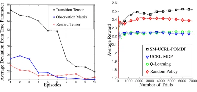
Finally, in the Appendix F, we report preliminary synthetic experiments that demonstrate su-periority of our method over existing RL methods such as Q-learning and UCRL for MDPs, and 2. This principle has been successfully used in a wide number of exploration–exploitation problems ranging from multi-armed bandit (Auer et al.,2002), linear contextual bandit (Abbasi-Yadkori et al.,2011), linear quadratic con-trol (Abbasi-Yadkori and Szepesv´ari,2011), and reinforcement learning (Ortner and Auer,2007;Jaksch et al.,2010).
also over purely exploratory methods such as random sampling, which randomly chooses actions independent of the observations. SM-UCRLconverges much faster and to a better solution. The so-lutions relying on the MDP assumption, directly work in the (high) dimensional observation space and perform poorly. In fact, they can even be worse than the random sampling policy baseline. In contrast, our method aims to find the lower dimensional latent space to derive the policy and this allowsUCRLto find a much better memoryless policy with vanishing regret.
1.2. Related Work
While RL in MDPs has been widely studied (Kearns and Singh, 2002;Brafman and Tennenholtz,
2003;Bartlett and Tewari,2009;Jaksch et al.,2010), the design of effective exploration–exploration
strategies in POMDPs is still relatively unexplored. Ross et al. (2007) and Poupart and Vlassis
(2008) propose to integrate the problem of estimating the belief state into a model-based Bayesian RL approach, where a distribution over possible MDPs is updated over time. The proposed algo-rithms are such that the Bayesian inference can be done accurately and at each step, a POMDP is sampled from the posterior and the corresponding optimal policy is executed. While the resulting methods implicitly balance exploration and exploitation, no theoretical guarantee is provided about their regret and their algorithmic complexity requires the introduction of approximation schemes for both the inference and the planning steps. An alternative to model-based approaches is to adapt model-free algorithms, such as Q-learning, to the case of POMDPs. Perkins (2002) proposes a Monte-Carlo approach to action-value estimation and it shows convergence to locally optimal mem-oryless policies. While this algorithm has the advantage of being computationally efficient, local optimal policies may be arbitrarily suboptimal and thus suffer a linear regret.
An alternative approach to solve POMDPs is to use policy search methods, which avoid esti-mating value functions and directly optimize the performance by searching in a given policy space, which usually contains memoryless policies (see e.g., (Ng and Jordan, 2000),(Baxter and Bartlett,
2001),(Poupart and Boutilier, 2003; Bagnell et al., 2004)). Beside its practical success in offline
problems, policy search has been successfully integrated with efficient exploration–exploitation techniques and shown to achieve small regret (Gheshlaghi-Azar et al.,2013,2014). Nonetheless, the performance of such methods is severely constrained by the choice of the policy space, which may not contain policies with good performance.
Matrix decomposition methods have been previously used in the more general setting of pre-dictive state representation (PSRs) (Boots et al., 2011) to reconstruct the structure of the dynami-cal system. Despite the generality of PSRs, the proposed model relies on strong assumptions on the dynamics of the system and it does not have any theoretical guarantee about its performance.
Gheshlaghi azar et al.(2013) used spectral tensor decomposition methods in the multi-armed bandit
framework to identify the hidden generative model of a sequence of bandit problems and showed that this may drastically reduce the regret.
Krishnamurthy et al.(2016) recently analyzed the problem of learning in contextual-MDPs and
proved sample complexity bounds polynomial in the capacity of the policy space, the number of states, and the horizon. While their objective is to minimize the regret over a finite horizon, we instead consider the infinite horizon problem. It is an open question to analyze and modify our spectral UCRL algorithm for the finite horizon problem. As stated earlier, contextual MDPs are a special class of POMDPs for which memoryless policies are optimal. While they assume that the
xt xt+1 xt+2
yt yt+1
rt rt+1
at at+1
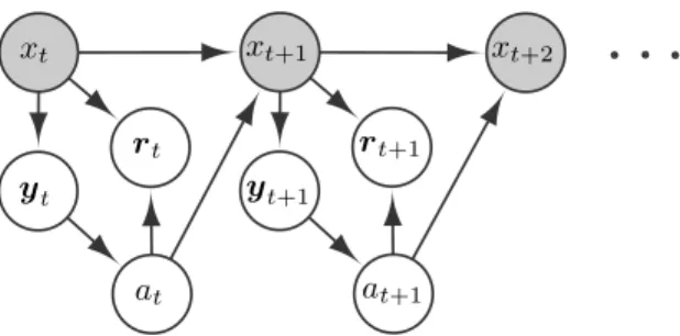
Figure 1: Graphical model of a POMDP under memoryless policies.
samples are drawn from a contextual MDP, we can handle a much more general class of POMDPs, and we minimize regret with respect to the best memoryless policy for the given POMDP.
Finally, a related problem is considered byOrtner et al.(2014), where a series of possible rep-resentations based on observation histories is available to the agent but only one of them is actually Markov. AUCRL-like strategy is adopted and shown to achieve near-optimal regret.
In this paper, we focus on the learning problem, while we consider access to an optimization oracle to compute the optimal memoryless policy. The problem of planning in general POMDPs is intractable (PSPACE-complete for finite horizon (Papadimitriou and Tsitsiklis, 1987) and uncom-putable for infinite horizon (Madani,1998)).Many exact, approximate, and heuristic methods have been proposed to compute the optimal policy (see Spaan (2012) for a recent survey). An alter-native approach is to consider memoryless policies which directly map observations (or a finite history) to actions (Littman, 1994; Singh et al., 1994; Li et al., 2011). While deterministic poli-cies may perform poorly, stochastic memoryless polipoli-cies are shown to be near-optimal in many domains (Barto et al.,1983;Loch and Singh,1998;Williams and Singh,1998) and even optimal in the specific case of contextual MDPs (Krishnamurthy et al.,2016). Although computing the optimal stochastic memoryless policy is still NP-hard (Littman,1994), several model-based and model-free methods are shown to converge to nearly-optimal policies with polynomial complexity under some conditions on the POMDP (Jaakkola et al.,1995;Li et al.,2011). In this work, we employ memo-ryless policies and prove regret bounds for reinforcement learning of POMDPs. The above works suggest that focusing to memoryless policies may not be a restrictive limitation in practice.
1.3. Paper Organization
The paper is organized as follows. Sect.2introduces the notation (summarized also in a table in Sect.6) and the technical assumptions concerning the POMDP and the space of memoryless policies that we consider. Sect.3introduces the spectral method for the estimation of POMDP parameters together with Thm.3. In Sect.4, we outline SM-UCRL where we integrate the spectral method into an exploration–exploitation strategy and we prove the regret bound of Thm.4. Sect.5draws conclusions and discuss possible directions for future investigation. The proofs are reported in the appendix together with preliminary empirical results showing the effectiveness of the proposed method.
2. Preliminaries
A POMDP M is a tuple %X , A, Y, R, fT, fR, fO&, where X is a finite state space with cardinality
|X | = X, A is a finite action space with cardinality |A| = A, Y is a finite observation space with cardinality |Y| = Y , and R is a finite reward space with cardinality |R| = R and largest reward rmax. For notation convenience, we use a vector notation for the elements in Y and R, so
that y ∈ RY and r ∈ RRare indicator vectors with entries equal to 0 except a 1 in the position
corresponding to a specific element in the set (e.g., y = enrefers to the n-th element in Y). We use
i, j∈ [X] to index states, k, l ∈ [A] for actions, m ∈ [R] for rewards, and n ∈ [Y ] for observations. Finally, fT denotes the transition density, so that fT(x#|x, a) is the probability of transition to x#
given the state-action pair (x, a), fRis the reward density, so that fR(r|x, a) is the probability of
receiving the reward in R corresponding to the value of the indicator vector r given the state-action pair (x, a), and fO is the observation density, so that fO(y|x) is the probability of receiving the
observation in Y corresponding to the indicator vector y given the state x. Whenever convenient, we use tensor forms for the density functions such that
Ti,j,l=P[xt+1 = j|xt= i, at= l] = fT(j|i, l), s.t. T ∈ RX×X×A
On,i=P[y = en|x = i] = fO(en|i), s.t. O∈ RY×X
Γi,l,m=P[r = em|x = i, a = l] = fR(em|i, l), s.t. Γ∈ RX×A×R.
We also denote by T:,j,lthe fiber (vector) in RX obtained by fixing the arrival state j and action l
and by T:,:,l∈ RX×Xthe transition matrix between states when using action l. The graphical model
associated to the POMDP is illustrated in Fig.1.
We focus on stochastic memoryless policies which map observations to actions and for any pol-icy π we denote by fπ(a|y) its density function. We denote by P the set of all stochastic memoryless
policies that have a non-zero probability to explore all actions: P = {π : min
y mina fπ(a|y) > πmin}.
Acting according to a policy π in a POMDP M defines a Markov chain characterized by a transition density fT,π(x#|x) = * a * y fπ(a|y)fO(y|x)fT(x#|x, a),
and a stationary distribution ωπ over states such that ωπ(x) =+x"fT,π(x#|x)ωπ(x#). The expected
average reward performance of a policy π is η(π; M ) =*
x
ωπ(x)rπ(x),
where rπ(x)is the expected reward of executing policy π in state x defined as
rπ(x) = * a * y fO(y|x)fπ(a|y)r(x, a),
and r(x, a) = +rrfR(r|x, a) is the expected reward for the state-action pair (x, a). The best
stochastic memoryless policy in P is π+ = arg max
π∈P η(π; M )and we denote by η
its average reward.3 Throughout the paper we assume that we have access to an optimization oracle returning the optimal policy π+ in P for any POMDP M. We need the following assumptions on
the POMDP M.
Assumption 1 (Ergodicity) For any policy π ∈ P, the corresponding Markov chain fT,π is
er-godic, so ωπ(x) > 0for all states x ∈ X .
We further characterize the Markov chains that can be generated by the policies in P. For any ergodic Markov chain with stationary distribution ωπ, let f1→t(xt|x1)by the distribution over states
reached by a policy π after t steps starting from an initial state x1. The inverse mixing time ρmix,π(t)
of the chain is defined as
ρmix,π(t) = sup x1
!f1→t(·|x1)− ωπ!TV,
where ! · !TV is the total-variation metric. Kontorovich et al. (2014) show that for any ergodic
Markov chain the mixing time can be bounded as
ρmix,π(t)≤ G(π)θt−1(π),
where 1 ≤ G(π) < ∞ is the geometric ergodicity and 0 ≤ θ(π) < 1 is the contraction coefficient of the Markov chain generated by policy π.
Assumption 2 (Full Column-Rank) The observation matrix O ∈ RY×X is full column rank.
and define
This assumption guarantees that the distribution fO(·|x) in a state x (i.e., a column of the matrix
O) is not the result of a linear combination of the distributions over other states. We show later that this is a sufficient condition to recover fO since it makes all states distinguishable from the
observations and it also implies that Y ≥ X. Notice that POMDPs have been often used in the opposite scenario (X * Y ) in applications such as robotics, where imprecise sensors prevents from distinguishing different states. On the other hand, there are many domains in which the number of observations may be much larger than the set of states that define the dynamics of the system. A typical example is the case of spoken dialogue systems (Atrash and Pineau,2006;Png et al.,2012), where the observations (e.g., sequences of words uttered by the user) is much larger than the state of the conversation (e.g., the actual meaning that the user intended to communicate). A similar scenario is found in medical applications (Hauskrecht and Fraser, 2000), where the state of a patient (e.g., sick or healthy) can produce a huge body of different (random) observations. In these problems it is crucial to be able to reconstruct the underlying small state space and the actual dynamics of the system from the observations.
Assumption 3 (Invertible) For any action a ∈ [A], the transition matrix T:,:,a ∈ RX×X is
invert-ible.
Similar to the previous assumption, this means that for any action a the distribution fT(·|x, a)
cannot be obtained as linear combination of distributions over other states, and it is a sufficient condition to be able to recover the transition tensor. Both Asm. 2and 3are strictly related to the assumptions introduced byAnandkumar et al. (2014) for tensor methods in HMMs. In Sect.4we discuss how they can be partially relaxed.
3. We use π+ rather than π∗to recall the fact that we restrict the attention to P and the actual optimal policy for a
3. Learning the Parameters of the POMDP
In this section we introduce a novel spectral method to estimate the POMDP parameters fT, fO,
and fR. A stochastic policy π is used to generate a trajectory (y1, a1, r1, . . . , yN, aN, rN)of N
steps. We need the following assumption that, together with Asm.1, guarantees that all states and actions are constantly visited.
Assumption 4 (Policy Set) The policy π belongs to P.
Similar to the case of HMMs, the key element to apply the spectral methods is to construct a multi-view model for the hidden states. Despite its similarity, the spectral method developed for HMM byAnandkumar et al.(2014) cannot be directly employed here. In fact, in HMMs the state transition and the observations only depend on the current state. On the other hand, in POMDPs the probability of a transition to state x# not only depends on x, but also on action a. Since the action is
chosen according to a memoryless policy π based on the current observation, this creates an indirect dependency of x#on observation y, which makes the model more intricate.
3.1. The multi-view model
We estimate POMDP parameters for each action l ∈ [A] separately. Let t ∈ [2, N − 1] be a step at which at = l, we construct three views (at−1, yt−1, rt−1), (yt, rt), and (yt+1) which all contain
observable elements. As it can be seen in Fig.1, all three views provide some information about the hidden state xt (e.g., the observation yt−1 triggers the action at−1, which influence the transition
to xt). A careful analysis of the graph of dependencies shows that conditionally on xt, atall the
views are independent. For instance, let us consider yt and yt+1. These two random variables
are clearly dependent since yt influences action at, which triggers a transition to xt+1 that emits
an observation yt+1. Nonetheless, it is sufficient to condition on the action at = l to break the
dependency and make ytand yt+1independent. Similar arguments hold for all the other elements
in the views, which can be used to recover the latent variable xt. More formally, we encode the
triple (at−1, yt−1, rt−1)into a vector v(l)1,t ∈ RA·Y ·R, so that view v (l)
1,t = eswhenever at−1 = k,
yt−1 = en, and rt−1 = em for a suitable mapping between the index s ∈ {1, . . . , A · Y · R} and
the indices (k, n, m) of the action, observation, and reward. Similarly, we proceed for v(l)
2,t ∈ RY·R
and v(l)
3,t ∈ RY. We introduce the three view matrices V (l)
ν with ν ∈ {1, 2, 3} associated with action
ldefined as V1(l)∈ RA·Y ·R×X, V2(l)∈ RY·R×X, and V(l)
3 ∈ RY×X such that [V1(l)]s,i=P,v(l)1 = es|x2 = i-= [V1(l)](n,m,k),i=P , y1 = en, r1 = em, a1 = k|x2 = i-, [V2(l)]s,i=P , v(l)2 = es|x2 = i, a2 = l -= [V2(l)](n",m"),i=P , y2 = en", r2 = em"|x2 = i, a2 = l-, [V3(l)]s,i=P , v(l)3 = es|x2 = i, a2 = l -= [V3(l)]n"",i=P , y3= en""|x2 = i, a2 = l -.
In the following we denote by µ(l)ν,i= [Vν(l)]:,ithe ith column of the matrix Vν(l)for any ν ∈ {1, 2, 3}.
Notice that Asm.2and Asm. 3imply that all the view matrices are full column rank. As a result, we can construct a multi-view model that relates the spectral decomposition of the second and third moments of the (modified) views with the columns of the third view matrix.
Proposition 1 (Thm. 3.6 in (Anandkumar et al.,2014)) Let K(l) ν,ν" =E & v(l)ν ⊗ v(l)ν" ' be the cor-relation matrix between views ν and ν#and K†is its pseudo-inverse. We define a modified version
of the first and second views as "
v(l)1 := K3,2(l)(K1,2(l))†v(l)1 , "v(l)2 := K3,1(l)(K2,1(l))†v(l)2 . (1) Then the second and third moment of the modified views have a spectral decomposition as
M2(l)=E&"v(l)1 ⊗ "v (l) 2 ' = X * i=1
ωπ(l)(i)µ(l)3,i⊗ µ(l)3,i, (2)
M3(l)=E&"v1(l)⊗ "v(l)2 ⊗ v(l)3 '=
X
*
i=1
ω(l)π (i)µ(l)3,i⊗ µ(l)3,i⊗ µ(l)3,i, (3) where ⊗ is the tensor product and ωπ(l)(i) =P[x = i|a = l] is the state stationary distribution of π
conditioned on action l being selected by policy π. Notice that under Asm. 1 and4, ω(l)
π (i)is always bounded away from zero. Given M2(l) and
M3(l) we can recover the columns of the third view µ(l)3,i directly applying the standard spectral decomposition method ofAnandkumar et al.(2012). We need to recover the other views from V(l)
3 .
From the definition of modified views in Eq.1we have µ(l)3,i=E&"v1|x2 = i, a2 = l ' = K3,2(l)(K1,2(l))†E&v1|x2= i, a2 = l ' = K3,2(l)(K1,2(l))†µ(l)1,i, µ(l)3,i=E&"v2|x2 = i, a2 = l ' = K3,1(l)(K2,1(l))†E&v2|x2= i, a2 = l ' = K3,1(l)(K2,1(l))†µ(l)2,i. (4) Thus, it is sufficient to invert (pseudo invert) the two equations above to obtain the columns of both the first and second view matrices. This process could be done in any order, e.g., we could first estimate the second view by applying a suitable symmetrization step (Eq.1) and recovering the first and the third views by reversing similar equations to Eq.4. On the other hand, we cannot repeat the symmetrization step multiple times and estimate the views independently (i.e., without inverting Eq.4). In fact, the estimates returned by the spectral method are consistent “up to a suitable permutation” on the indexes of the states. While this does not pose any problem in computing one single view, if we estimated two views independently, the permutation may be different, thus making them non-consistent and impossible to use in recovering the POMDP parameters. On the other hand, estimating first one view and recovering the others by inverting Eq.4guarantees the consistency of the labeling of the hidden states.
3.2. Recovery of POMDP parameters Once the views {V(l)
ν }3ν=2 are computed from M (l)
2 and M (l)
3 , we can derive fT, fO, and fR. In
particular, all parameters of the POMDP can be obtained by manipulating the second and third view as illustrated in the following lemma.
Lemma 2 Given the views V(l) 2 and V
(l)
3 , for any state i ∈ [X] and action l ∈ [A], the POMDP
parameters are obtained as follows. For any reward m ∈ [R] the reward density is fR(em"|i, l) =
Y
*
n"=1
for any observation n# ∈ [Y ] the observation density is fO(l)(en"|i) = R * m"=1 [V2(l)](n",m"),i fπ(l|en")ρ(i, l), (6) with ρ(i, l) = R * m"=1 Y * n"=1 [V2(l)](n",m"),i fπ(l|en") = 1 P(a2 = l|x2 = i) . Finally, each second mode of the transition tensor T ∈ RX×X×Ais obtained as
[T ]i,:,l = O†[V3(l)]:,i, (7)
where O†is the pseudo-inverse of matrix observation O and f
T(·|i, l) = [T ]i,:,l.
In the previous statement we use f(l)
O to denote that the observation model is recovered from
the view related to action l. While in the exact case, all fO(l)are identical, moving to the empirical version leads to A different estimates, one for each action view used to compute it. Among them, we will select the estimate with the better accuracy.
Empirical estimates of POMDP parameters. In practice, M(l)
2 and M (l)
3 are not available and
need to be estimated from samples. Given a trajectory of N steps obtained executing policy π, let T (l) = {t ∈ [2, N − 1] : at = l} be the set of steps when action l is played, then we collect all
the triples (at−1, yt−1, rt−1), (yt, rt)and (yt+1)for any t ∈ T (l) and construct the corresponding
views v(l)1,t, v (l) 2,t, v
(l)
3,t. Then we symmetrize the views using empirical estimates of the covariance
matrices and build the empirical version of Eqs.2and3using N(l) = |T (l)| samples, thus obtaining . M2(l)= 1 N (l) * t∈Tl "v(l)1,t⊗ "v (l) 2,t, M. (l) 3 = 1 N (l) * t∈Tl "v(l)1,t⊗ "v (l) 2,t⊗ v (l) 3,t. (8)
Given the resulting .M2(l) and .M3(l), we apply the spectral tensor decomposition method to recover an empirical estimate of the third view !V3(l)and invert Eq.4(using estimated covariance matrices) to obtain !V2(l). Finally, the estimates !fO, !fT, and !fRare obtained by plugging the estimated views
!
Vνin the process described in Lemma2.
Spectral methods indeed recover the factor matrices up to a permutation of the hidden states. In this case, since we separately carry out spectral decompositions for different actions, we recover permuted factor matrices. Since the observation matrix O is common to all the actions, we use it to align these decompositions. Let’s define dO
dO =: min
x,x" !fO(·|x) − fO(·|x
#)! 1
Actually, dO is the minimum separability level of matrix O. When the estimation error over
columns of matrix O are less than 4dO, then one can come over the permutation issue by matching
Algorithm 1 Estimation of the POMDP parameters. The routineTENSORDECOMPOSITIONrefers to
the spectral tensor decomposition method ofAnandkumar et al.(2012).
Input:
Policy density fπ, number of states X
Trajectory %(y1, a1, r1), (y2, a2, r2), . . . , (yN, aN, rN)&
Variables:
Estimated second and third views !V2(l), and !V (l)
3 for any action l ∈ [A]
Estimated observation, reward, and transition models !fO, !fR, !fT
for l = 1, . . . , A do
Set T (l) = {t ∈ [N − 1] : at= l} and N(l) = |T (l)|
Construct views v(l)
1,t= (at−1, yt−1, rt−1), v2,t(l) = (yt, rt), v(l)3,t= yt+1 for any t ∈ T (l)
Compute covariance matrices !K3,1(l), !K (l) 2,1, !K (l) 3,2as ! Kν,ν(l)" = 1 N (l) * t∈T (l) v(l)ν,t⊗ v (l) ν",t; ν, ν#∈ {1, 2, 3}
Compute modified views "v(l) 1,t:= !K (l) 3,2( !K (l) 1,2)†v1, "v(l)2,t:= !K (l) 3,1( !K (l) 2,1)†v (l) 2,t for any t ∈ T (l)
Compute second and third moments . M2(l)= 1 N (l) * t∈Tl "v(l)1,t⊗ "v (l) 2,t, M. (l) 3 = 1 N (l) * t∈Tl "v(l)1,t⊗ "v (l) 2,t⊗ v (l) 3,t
Compute !V3(l)= TENSORDECOMPOSITION( .M (l) 2 , .M (l) 3 ) Compute !µ(l) 2,i= !K (l) 1,2( !K (l) 3,2)†!µ (l)
3,i for any i ∈ [X]
Compute !f (em|i, l) =+Yn"=1[ !V (l)
2 ](n",m),i for any i ∈ [X], m ∈ [R]
Compute ρ(i, l) =+R m"=1
+Y n"=1
[V2(l)](n",m" ),i
fπ(l|en") for any i ∈ [X], n ∈ [Y ]
Compute !fO(l)(en|i) =+Rm"=1
[V2(l)](n,m"),i
fπ(l|en)ρ(i,l) for any i ∈ [X], n ∈ [Y ]
end for
Compute bounds B(l) O
Set l∗= arg min
lB(l)O, !fO= !fl
∗
O and construct matrix [ !O]n,j= !fO(en|j)
Reorder columns of matrices !V2(l)and !V3(l)such that matrix O(l)and O(l∗)match, ∀l ∈ [A]4
for i ∈ [X], l ∈ [A] do
Compute [T ]i,:,l= !O†[ !V3(l)]:,i
end for
Return: !fR, !fT, !fO, BR, BT, BO
columns of Ol matrices. In T condition is reflected as a condition that the number of samples for
each action has to be larger some number.
The overall method is summarized in Alg.1. The empirical estimates of the POMDP parameters enjoy the following guarantee.
Theorem 3 (Learning Parameters) Let !fO, !fT, and !fRbe the estimated POMDP models using a
covariance matrix Kν,ν", with ν, ν#∈ {1, 2, 3}, and by σmin(Vν(l))the smallest singular value of the
view matrix V(l)
ν (strictly positive under Asm.2and Asm.3), and we define ω(l)min= minx∈X ω(l)π (x)
(strictly positive under Asm.1). If for any action l ∈ [A], the number of samples N(l) satisfies the condition N (l)≥ max / 4 (σ3,1(l))2, 16CO2Y R λ(l)2d2 O , G(π) 2√2+1 1−θ(π) ωmin(l) min ν∈{1,2,3}{σ 2 min(V (l) ν )} 2 Θ(l) 6 log(2(Y 2+ AY R) δ ) , (9) with Θ(l), defined in Eq275, and G(π), θ(π) are the geometric ergodicity and the contraction coef-ficients of the corresponding Markov chain induced by π, then for any δ ∈ (0, 1) and for any state i∈ [X] and action l ∈ [A] we have
! !fO(l)(·|i)−fO(·|i)!1 ≤ B(l)O := CO λ(l) $ Y R log(1/δ) N (l) , (10) ! !fR(·|i, l) − fR(·|i, l)!1 ≤ BR(l):= CR λ(l) $ Y R log(1/δ) N (l) , (11) ! !fT(·|i, l)−fT(·|i, l)!2 ≤ BT(l):= CT λ(l) $ Y RX2log(1/δ) N (l) , (12)
with probability 1 − 6(Y2+ AY R)Aδ (w.r.t. the randomness in the transitions, observations, and
policy), where CO, CR, and CT are numerical constants and
λ(l)= σmin(O)(πmin(l) )2σ1,3(l)(ω (l)
minν min ∈{1,2,3}{σ
2
min(Vν(l))})3/2. (13)
Finally, we denote by !fOthe most accurate estimate of the observation model, i.e., the estimate !f(l
∗)
O
such that l∗= arg min
l∈[A]B(l)O and we denote by BOits corresponding bound.
Remark 1 (consistency and dimensionality). All previous errors decrease with a rate "O(1/7N (l)), showing the consistency of the spectral method, so that if all the actions are repeatedly tried over time, the estimates converge to the true parameters of the POMDP. This is in contrast with EM-based methods which typically get stuck in local maxima and return biased estimators, thus preventing from deriving confidence intervals.
The bounds in Eqs. 10, 11, 12 on !fO, !fR and !fT depend on X, Y , and R (and the number
of actions only appear in the probability statement). The bound in Eq.12on !fT is worse than the
bounds for !fRand !fOin Eqs.10,11by a factor of X2. This seems unavoidable since !fRand !fOare
5. We do not report the explicit definition of Θ(l)here because it contains exactly the same quantities, such as ω(l) min,
the results of the manipulation of the matrix V2(l)with Y · R columns, while estimating !fT requires
working on both V2(l)and V (l)
3 . In addition, to come up with upper bound for !fT, more complicated
bound derivation is needed and it has one step of Frobenious norms to +2 norm transformation. The derivation procedure for !fT is more complicated compared to !fOand !fRand adds the term X to
the final bound. (Appendix.C)
Remark 2 (POMDP parameters and policy π). In the previous bounds, several terms depend on the structure of the POMDP and the policy π used to collect the samples:
• λ(l)captures the main problem-dependent terms. While K1,2and K1,3 are full column-rank
matrices (by Asm.2and3), their smallest non-zero singular values influence the accuracy of the (pseudo-)inversion in the construction of the modified views in Eq.1and in the compu-tation of the second view from the third using Eq.4. Similarly the presence of σmin(O)is
justified by the pseudo-inversion of O used to recover the transition tensor in Eq.7. Finally, the dependency on the smallest singular values σ2
min(V (l)
ν )is due to the tensor decomposition
method (see App.Jfor more details).
• A specific feature of the bounds above is that they do not depend on the state i and the number of times it has been explored. Indeed, the inverse dependency on ωmin(l) in the condition on N (l)in Eq. 9 implies that if a state j is poorly visited, then the empirical estimate of any other state i may be negatively affected. This is in striking contrast with the fully observable case where the accuracy in estimating, e.g., the reward model in state i and action l, simply depends on the number of times that state-action pair has been explored, even if some other states are never explored at all. This difference is intrinsic in the partial observable nature of the POMDP, where we reconstruct information about the states (i.e., reward, transition, and observation models) only from indirect observations. As a result, in order to have accurate estimates of the POMDP structure, we need to rely on the policy π and the ergodicity of the corresponding Markov chain to guarantee that the whole state space is covered.
• Under Asm.1the Markov chain fT,πis ergodic for any π ∈ P. Since no assumption is made
on the fact that the samples generated from π being sampled from the stationary distribution, the condition on N(l) depends on how fast the chain converge to ωπ and this is characterized
by the parameters G(π) and θ(π).
• If the policy is deterministic, then some actions would not be explored at all, thus leading to very inaccurate estimations (see e.g., the dependency on fπ(l|y) in Eq. 6). The inverse
dependency on πmin(defined in P) accounts for the amount of exploration assigned to every
actions, which determines the accuracy of the estimates. Furthermore, notice that also the singular values σ(l)1,3and σ(l)1,2depend on the distribution of the views, which in turn is partially determined by the policy π.
Notice that the first two terms are basically the same as in the bounds for spectral methods applied to HMM (Song et al.,2013), while the dependency on πminis specific to the POMDP case.
On the other hand, in the analysis of HMMs usually there is no dependency on the parameters G and θ because the samples are assumed to be drawn from the stationary distribution of the chain. Removing this assumption required developing novel results for the tensor decomposition process itself using extensions of matrix concentration inequalities for the case of Markov chain (not yet
Algorithm 2 TheSM-UCRLalgorithm.
Input: Confidence δ#
Variables:
Number of samples N(k)(l)
Estimated observation, reward, and transition models !fO(k), !fR(k), !fT(k) Initialize: t = 1, initial state x1, δ = δ#/N6, k = 1
while t < N do
Compute the estimated POMDP .M(k)with the Alg.1using N(k)(l)samples per action
Compute the set of admissible POMDPs M(k)using bounds in Thm.3
Compute the optimistic policy "π(k)= arg max
π∈PMmax∈M(k)η(π; M )
Set v(k)(l) = 0for all actions l ∈ [A]
while ∀l ∈ [A], v(k)(l) < 2N(k)(l)do
Execute at∼ f!π(k)(·|yt)
Obtain reward rt, observe next observation yt+1, and set t = t + 1
end while
Store N(k+1)(l) = max
k"≤kv(k")(l)samples for each action l ∈ [A]
Set k = k + 1 end while
in the stationary distribution). The overall analysis is reported in App. I and J. It worth to note that, Kontorovich et al. (2013), without stationary assumption, proposes new method to learn the transition matrix of HMM model given factor matrix O, and it provides theoretical bound over estimation errors.
4. SpectralUCRL
The most interesting aspect of the estimation process illustrated in the previous section is that it can be applied when samples are collected using any policy π in the set P. As a result, it can be integrated into any exploration-exploitation strategy where the policy changes over time in the attempt of minimizing the regret.
The algorithm. The SM-UCRLalgorithm illustrated in Alg. 2 is the result of the integration of the spectral method into a structure similar toUCRL(Jaksch et al.,2010) designed to optimize the exploration-exploitation trade-off. The learning process is split into episodes of increasing length. At the beginning of each episode k > 1 (the first episode is used to initialize the variables), an estimated POMDP .M(k) = (X, A, Y, R, !fT(k), !fR(k), !fO(k))is computed using the spectral method of Alg.1. Unlike in UCRL, SM-UCRLcannot use all the samples from past episodes. In fact, the distribution of the views v1, v2, v3depends on the policy used to generate the samples. As a result,
whenever the policy changes, the spectral method should be re-run using only the samples collected by that specific policy. Nonetheless we can exploit the fact that the spectral method is applied to each action separately. InSM-UCRLat episode k for each action l we use the samples coming from the past episode which returned the largest number of samples for that action. Let v(k)(l)be the number
of samples obtained during episode k for action l, we denote by N(k)(l) = max
k"<kv(k")(l)the
largest number of samples available from past episodes for each action separately and we feed them to the spectral method to compute the estimated POMDP .M(k)at the beginning of each episode k.
Given the estimated POMDP .M(k) and the result of Thm. 3, we construct the set M(k) of admissible POMDPs 8M = %X , A, Y, R, "fT, "fR, "fO& whose transition, reward, and observation
models belong to the confidence intervals (e.g., ! !fO(k)(·|i)− "fO(·|i)!1 ≤ BO for any state i). By
construction, this guarantees that the true POMDP M is included in M(k) with high probability.
Following the optimism in face of uncertainty principle used in UCRL, we compute the optimal memoryless policy corresponding to the most optimistic POMDP within M(k). More formally, we
compute6
"π(k)= arg max
π∈P Mmax∈M(k)η(π; M ). (14)
Intuitively speaking, the optimistic policy implicitly balances exploration and exploitation. Large confidence intervals suggest that .M(k)is poorly estimated and further exploration is needed. Instead of performing a purely explorative policy,SM-UCRLstill exploits the current estimates to construct the set of admissible POMDPs and selects the policy that maximizes the performance η(π; M) over all POMDPs in M(k). The choice of using the optimistic POMDP guarantees the "π(k) explores
more often actions corresponding to large confidence intervals, thus contributing the improve the estimates over time. After computing the optimistic policy, "π(k) is executed until the number of
samples for one action is doubled, i.e., v(k)(l)≥ 2N(k)(l). This stopping criterion avoids switching
policies too often and it guarantees that when an episode is terminated, enough samples are collected to compute a new (better) policy. This process is then repeated over episodes and we expect the optimistic policy to get progressively closer to the best policy π+ ∈ P as the estimates of the
POMDP get more and more accurate.
Regret analysis. We now study the regretSM-UCRLw.r.t. the best policy in P. While in general
π+may not be optimal, πminis usually set to a small value and oftentimes the optimal memoryless
policy itself is stochastic and it may actually be contained in P. Given an horizon of N steps, the regret is defined as RegN = N η+− N * t=1 rt, (15)
where rtis the random reward obtained at time t according to the reward model fRover the states
traversed by the policies performed over episodes on the actual POMDP. To restate, similar to the MDP case, the complexity of learning in a POMDP M is partially determined by its diameter, defined as
D := max
x,x"∈X ,a,a"∈Aminπ∈PE
&
τ (x#, a#|x, a; π)', (16) which corresponds to the expected passing time from a state x to a state x# starting with action a
and terminating with action a# and following the most effective memoryless policy π ∈ P. The
6. The computation of the optimal policy (within P) in the optimistic model may not be trivial. Nonetheless, we first notice that given an horizon N, the policy needs to be recomputed at most O(log N) times (i.e., number of episodes). Furthermore, if an optimization oracle to η(π; M) for a given POMDP M is available, then it is sufficient to ran-domly sample multiple POMDPs from M(k)(which is a computationally cheap operation), find their corresponding
best policy, and return the best among them. If enough POMDPs are sampled, the additional regret caused by this approximately optimistic procedure can be bounded as !O(√N ).
main difference w.r.t. to the diameter of the underlying MDP (see e.g.,Jaksch et al.(2010)) is that it considers the distance between state-action pairs using memoryless policies instead of state-based policies.
Before stating our main result, we introduce the worst-case version of the parameters char-acterizing Thm. 3. Let σ1,2,3 := min
l∈[A]minπ∈Pω (l) minν min ∈{1,2,3}σ 2 min(V (l)
ν ) be the worst smallest
non-zero singular value of the views for action l when acting according to policy π and let σ1,3 :=
min
l∈[A]minπ∈Pσmin(K (l)
1,3(π)) be the worst smallest non-zero singular value of the covariance matrix
K1,3(l)(π)between the first and third view for action l when acting according to policy π. Similarly, we define σ1,2. We also introduce ωmin:= min
l∈[A]x∈[X]min minπ∈Pω (l) π (x)and
N := max
l∈[A]maxπ∈P max
/ 4 (σ2 3,1) ,16C 2 OY R λ(l)2d2 O , G(π) 2√2+1 1−θ(π) ωminσ1,2,3 2 Θ(l) 6 log # 2(Y 2+ AY R) δ % , (17) which is a sufficient number of samples for the statement of Thm.3to hold for any action and any policy. Here Θ(l)is also model related parameter which is defined in Eq.36. Then we can prove the following result.
Theorem 4 (Regret Bound) Consider a POMDP M with X states, A actions, Y observations, R rewards, characterized by a diameter D and with an observation matrix O ∈ RY×X with smallest
non-zero singular value σX(O). We consider the policy space P, such that the worst smallest
non-zero value is σ1,2,3 (resp. σ1,3) and the worst smallest probability to reach a state is ωmin. If SM-UCRLis run over N steps and the confidence intervals of Thm.3are used with δ = δ#/N6in
constructing the plausible POMDPs 8M, then under Asm.1,2, and3it suffers from a total regret RegN ≤ C1
rmax
λ DX
3/27AY RN log(N/δ#) (18)
with probability 1 − δ#, where C
1 is numerical constants, and λ is the worst-case equivalent of
Eq.13defined as
λ = σmin(O)π2minσ1,3σ3/21,2,3. (19)
Remark 1 (comparison with MDPs). IfUCRLcould be run directly on the underlying MDP (i.e., as if the states where directly observable), then it would obtain a regret (Jaksch et al.,2010)
RegN ≤ CMDPDMDPX7AN log N ,
where
DMDP:= max
x,x"∈Xminπ E[τ(x #|x; π)],
with high probability. We first notice that the regret is of order "O(√N )in both MDP and POMDP bounds. This means that despite the complexity of POMDPs,SM-UCRLhas the same dependency
on the number of steps as in MDPs and it has a vanishing per-step regret. Furthermore, this de-pendency is known to be minimax optimal. The diameter D in general is larger than its MDP counterpart DMDP, since it takes into account the fact that a memoryless policy, that can only work
on observations, cannot be as efficient as a state-based policy in moving from one state to another. Although no lower bound is available for learning in POMDPs, we believe that this dependency is unavoidable since it is strictly related to the partial observable nature of POMDPs.
Remark 2 (dependency on POMDP parameters). The dependency on the number of actions is the same in both MDPs and POMDPs. On the other hand, moving to POMDPs naturally brings the dimensionality of the observation and reward models (Y ,X, and R respectively) into the bound. The dependency on Y and R is directly inherited from the bounds in Thm.3. The term X3/2 is
indeed the results of two terms; X and X1/2. The first term is the same as in MDPs, while the
second comes from the fact that the transition tensor is derived from Eq. 7. Finally, the term λ in Eq.18summarizes a series of terms which depend on both the policy space P and the POMDP structure. These terms are directly inherited from the spectral decomposition method used at the core ofSM-UCRLand, as discussed in Sect.3, they are due to the partial observability of the states and the fact that all (unobservable) states need to be visited often enough to be able to compute accurate estimate of the observation, reward, and transition models.
Remark 3 (computability of the confidence intervals). While it is a common assumption that the dimensionality X of the hidden state space is known as well as the number of actions, observations, and rewards, it is not often the case that the terms λ(l) appearing in Thm.3are actually available.
While this does not pose any problem for a descriptive bound as in Thm.3, inSM-UCRLwe actu-ally need to compute the bounds B(l)
O, B (l) R, and B
(l)
T to explicitly construct confidence intervals. This
situation is relatively common in many exploration–exploitation algorithms that require computing confidence intervals containing the range of the random variables or the parameters of their distri-butions in case of sub-Gaussian variables. In practice these values are often replaced by parameters that are tuned by hand and set to much smaller values than their theoretical ones. As a result, we can runSM-UCRLwith the terms λ(l)replaced by a fixed parameter. Notice that any inaccurate choice
in setting λ(l)would mostly translate into bigger multiplicative constants in the final regret bound
or in similar bounds but with smaller probability.
In general, computing confidence bound is a hard problem, even for simpler cases such as Markov chains?. Therefore finding upper confidence bounds for POMDP is challenging if we do not know its mixing properties. As it mentioned, another parameter is needed to compute upper confidence bound is λ(l)13. As it is described in, in practice, one can replace the coefficient λ(l)with some
constant which causes bigger multiplicative constant in final regret bound. Alternatively, one can estimate λ(l)from data. In this case, we add a lower order term to the regret which decays as 1
N.
Remark 4 (relaxation on assumptions). Both Thm.3and4rely on the observation matrix O ∈ RY×X being full column rank (Asm. 2). As discussed in Sect. 2 may not be verified in some
POMDPs where the number of states is larger than the number of observations (X > Y ). Nonethe-less, it is possible to correctly estimate the POMDP parameters when O is not full column-rank by exploiting the additional information coming from the reward and action taken at step t + 1. In
particular, we can use the triple (at+1, yt+1, rt+1)and redefine the third view V3(l) ∈ Rd×X as
[V3(l)]s,i=P(v(l)3 = es|x2 = i, a2 = l) = [V3(l)](n,m,k),i
=P(y3 = en, r3= em, a3= k|x2 = i, a2 = l),
and replace Asm.2with the assumption that the view matrix V3(l)is full column-rank, which ba-sically requires having rewards that jointly with the observations are informative enough to recon-struct the hidden state. While this change does not affect the way the observation and the reward models are recovered in Lemma2, (they only depend on the second view V2(l)), for the reconstruc-tion of the transireconstruc-tion tensor, we need to write the third view V3(l)as
[V3(l)]s,i= [V3(l)](n,m,k),i = X * j=1 P,y3 = en, r3= em, a3= k|x2= i, a2 = l, x3= j-P,x3= j|x2 = i, a2= l -= X * j=1 P,r3 = em|x3= j, a3 = k)P(a3= k|y3 = en-P,y3 = en|x3 = j-P,x3 = j|x2 = i, a2 = l -= fπ(k|en) X * j=1 fR(em|j, k)fO(en|j)fT(j|i, l),
where we factorized the three components in the definition of V(l)
3 and used the graphical model of
the POMDP to consider their dependencies. We introduce an auxiliary matrix W ∈ Rd×X such that
[W ]s,j= [W ](n,m,k),j= fπ(k|en)fR(em|j, k)fO(en|j),
which contain all known values, and for any state i and action l we can restate the definition of the third view as
W [T ]i,:,l= [V3(l)]:,i, (20)
which allows computing the transition model as [T ]i,:,l = W†[V3(l)]:,i, where W† is the
pseudo-inverse of W . While this change in the definition of the third view allows a significant relaxation of the original assumption, it comes at the cost of potentially worsening the bound on !fT in Thm.3.
In fact, it can be shown that
! "fT(·|i, l) − fT(·|i, l)!F≤BT# := max l"=1,...,A CTAY R λ(l") $ XA log(1/δ) N (l#) . (21)
Beside the dependency on multiplication of Y , R, and R, which is due to the fact that now V(l) 3
is a larger matrix, the bound for the transitions triggered by an action l scales with the number of samples from the least visited action. This is due to the fact that now the matrix W involves not only the action for which we are computing the transition model but all the other actions as well. As a result, if any of these actions is poorly visited, W cannot be accurately estimated is some
of its parts and this may negatively affect the quality of estimation of the transition model itself. This directly propagates to the regret analysis, since now we require all the actions to be repeatedly visited enough. The immediate effect is the introduction of a different notion of diameter. Let τM,π(l) the mean passage time between two steps where action l is chosen according to policy π ∈ P, we define
Dratio= max π∈P
maxl∈AτM,π(l)
minl∈AτM,π(l) (22)
as the diameter ratio, which defines the ratio between maximum mean passing time between choos-ing an action and chooschoos-ing it again, over its minimum. As it mentioned above, in order to have an accurate estimate of fT all actions need to be repeatedly explored. The Dratiois small when each
action is executed frequently enough and it is large when there is at least one action that is executed not as many as others. Finally, we obtain
RegN ≤ "O
(rmax
λ 7
Y RDratioN log N X3/2A(D + 1)
) .
While at first sight this bound is clearly worse than in the case of stronger assumptions, notice that λnow contains the smallest singular values of the newly defined views. In particular, as V3(l) is larger, also the covariance matrices Kν,ν" are bigger and have larger singular values, which could
significantly alleviate the inverse dependency on σ1,2 and σ2,3. As a result, relaxing Asm.2may
not necessarily worsen the final bound since the bigger diameter may be compensated by better dependencies on other terms. We leave a more complete comparison of the two configurations (with or without Asm.2) for future work.
5. Conclusion
We introduced a novel RL algorithm for POMDPs which relies on a spectral method to consis-tently identify the parameters of the POMDP and an optimistic approach for the solution of the exploration–exploitation problem. For the resulting algorithm we derive confidence intervals on the parameters and a minimax optimal bound for the regret.
This work opens several interesting directions for future development. 1)SM-UCRL cannot accumulate samples over episodes since Thm.3requires samples to be drawn from a fixed policy. While this does not have a very negative impact on the regret bound, it is an open question how to apply the spectral method to all samples together and still preserve its theoretical guarantees. 2) While memoryless policies may perform well in some domains, it is important to extend the current approach to bounded-memory policies. 3) The POMDP is a special case of the predictive state representation (PSR) model Littman et al. (2001), which allows representing more sophisticated dynamical systems. Given the spectral method developed in this paper, a natural extension is to apply it to the more general PSR model and integrate it with an exploration–exploitation algorithm to achieve bounded regret.
6. Table of Notation
POMDP Notation (Sect.2) e indicator vector
M POMDP model
X , X, x, (i, j) state space, cardinality, element, indices
Y, Y, y, n observation space, cardinality, indicator element, index A, A, a, (l, k) action space, cardinality, element, indices
R, R, r, r, m, rmax reward space, cardinality, element, indicator element, index, largest value
fT(x#|x, a), T transition density from state x to state x# given action a and transition tensor
fO(y|x), O observation density of indicator y given state x and observation matrix
fR(r|x, a), Γ reward density of indicator r given pair of state-action and reward tensor
π, fπ(a|y), Π policy, policy density of action a given observation indicator y and policy matrix
πmin, P smallest element of policy matrix and set of stochastic memoryless policies
fπ,T(x#|x) Markov chain transition density for policy π on a POMDP with transition density fT
ωπ, ω(l)π stationary distribution over states given policy π and conditional on action l
η(π, M ) expected average reward of policy π in POMDP M η+ best expected average reward over policies in P
POMDP Estimation Notation (Sect.3) ν ∈ {1, 2, 3} index of the views
v(l)ν,t, V (l)
ν νth view and view matrix at time t given at= l
Kν,ν(l)", σ
(l)
ν,ν" covariance matrix of views ν, ν#and its smallest non-zero singular value given action l
M2(l), M (l)
3 second and third order moments of the views given middle action l
! fO(l), !f
(l) R , !f
(l)
T estimates of observation, reward, and transition densities for action l
N, N(l) total number of samples and number of samples from action l CO, CR, CT numerical constants
BO, BR, BT upper confidence bound over error of estimated fO, fR, fT
SM-UCRL (Sect.4) RegN cumulative regret
D POMDP diameter k index of the episode !
fT(k), !fR(k), !fO(k), .M(k) estimated parameters of the POMDP at episode k
M(k) set of plausible POMDPs at episode k
v(k)(l) number of samples from action l in episode k
N(k)(l) maximum number of samples from action l over all episodes before k
"π(k) optimistic policy executed in episode k
N min. number of samples to meet the condition in Thm.3for any policy and any action σν,ν" worst smallest non-zero singular value of covariance Kν,ν(l)" for any policy and action
References
Yasin Abbasi-Yadkori and Csaba Szepesv´ari. Regret bounds for the adaptive control of linear quadratic systems. In COLT, pages 1–26, 2011.
Yasin Abbasi-Yadkori, D´avid P´al, and Csaba Szepesv´ari. Improved algorithms for linear stochastic bandits. In Advances in Neural Information Processing Systems 24 - NIPS, pages 2312–2320, 2011.
Animashree Anandkumar, Daniel Hsu, and Sham M Kakade. A method of moments for mixture models and hidden markov models. arXiv preprint arXiv:1203.0683, 2012.
Animashree Anandkumar, Rong Ge, Daniel Hsu, Sham M Kakade, and Matus Telgarsky. Tensor decompositions for learning latent variable models. The Journal of Machine Learning Research, 15(1):2773–2832, 2014.
A. Atrash and J. Pineau. Efficient planning and tracking in pomdps with large observation spaces. In AAAI Workshop on Statistical and Empirical Approaches for Spoken Dialogue Systems, 2006. Peter Auer, Nicol`o Cesa-Bianchi, and Paul Fischer. Finite-time analysis of the multiarmed bandit
problem. Machine Learning, 47(2-3):235–256, 2002.
Peter Auer, Thomas Jaksch, and Ronald Ortner. Near-optimal regret bounds for reinforcement learning. In Advances in neural information processing systems, pages 89–96, 2009.
J. A. Bagnell, Sham M Kakade, Jeff G. Schneider, and Andrew Y. Ng. Policy search by dynamic programming. In S. Thrun, L.K. Saul, and B. Sch¨olkopf, editors, Advances in Neural Information Processing Systems 16, pages 831–838. MIT Press, 2004.
Peter L. Bartlett and Ambuj Tewari. REGAL: A regularization based algorithm for reinforcement learning in weakly communicating MDPs. In Proceedings of the 25th Annual Conference on Uncertainty in Artificial Intelligence, 2009.
A.G. Barto, R.S. Sutton, and C.W. Anderson. Neuronlike adaptive elements that can solve difficult learning control problems. Systems, Man and Cybernetics, IEEE Transactions on, SMC-13(5): 834–846, Sept 1983. ISSN 0018-9472. doi: 10.1109/TSMC.1983.6313077.
Jonathan Baxter and Peter L. Bartlett. Infinite-horizon policy-gradient estimation. J. Artif. Int. Res., 15(1):319–350, November 2001. ISSN 1076-9757.
D. Bertsekas and J. Tsitsiklis. Neuro-Dynamic Programming. Athena Scientific, 1996.
Byron Boots, Sajid M Siddiqi, and Geoffrey J Gordon. Closing the learning-planning loop with predictive state representations. The International Journal of Robotics Research, 30(7):954–966, 2011.
Ronen I Brafman and Moshe Tennenholtz. R-max-a general polynomial time algorithm for near-optimal reinforcement learning. The Journal of Machine Learning Research, 3:213–231, 2003.
Wei Chen, Yajun Wang, and Yang Yuan. Combinatorial multi-armed bandit: General framework and applications. In Sanjoy Dasgupta and David Mcallester, editors, Proceedings of the 30th International Conference on Machine Learning (ICML-13), volume 28, pages 151–159. JMLR Workshop and Conference Proceedings, 2013.
Arthur P Dempster, Nan M Laird, and Donald B Rubin. Maximum likelihood from incomplete data via the em algorithm. Journal of the royal statistical society. Series B (methodological), pages 1–38, 1977.
M. Gheshlaghi-Azar, A. Lazaric, and E. Brunskill. Regret bounds for reinforcement learning with policy advice. In Proceedings of the European Conference on Machine Learning (ECML’13), 2013.
M. Gheshlaghi-Azar, A. Lazaric, and E. Brunskill. Resource-efficient stochastic optimization of a locally smooth function under correlated bandit feedback. In Proceedings of the Thirty-First International Conference on Machine Learning (ICML’14), 2014.
Mohammad Gheshlaghi azar, Alessandro Lazaric, and Emma Brunskill. Sequential transfer in multi-armed bandit with finite set of models. In C.J.C. Burges, L. Bottou, M. Welling, Z. Ghahra-mani, and K.Q. Weinberger, editors, Advances in Neural Information Processing Systems 26, pages 2220–2228. Curran Associates, Inc., 2013.
Milos Hauskrecht and Hamish Fraser. Planning treatment of ischemic heart disease with partially observable markov decision processes. Artificial Intelligence in Medicine, 18(3):221 – 244, 2000. ISSN 0933-3657.
Tommi Jaakkola, Satinder P. Singh, and Michael I. Jordan. Reinforcement learning algorithm for partially observable markov decision problems. In Advances in Neural Information Processing Systems 7, pages 345–352. MIT Press, 1995.
Thomas Jaksch, Ronald Ortner, and Peter Auer. Near-optimal regret bounds for reinforcement learning. J. Mach. Learn. Res., 11:1563–1600, August 2010. ISSN 1532-4435.
Michael Kearns and Satinder Singh. Near-optimal reinforcement learning in polynomial time. Ma-chine Learning, 49(2-3):209–232, 2002.
Aryeh Kontorovich, Boaz Nadler, and Roi Weiss. On learning parametric-output hmms. arXiv preprint arXiv:1302.6009, 2013.
Aryeh Kontorovich, Roi Weiss, et al. Uniform chernoff and dvoretzky-kiefer-wolfowitz-type in-equalities for markov chains and related processes. Journal of Applied Probability, 51(4):1100– 1113, 2014.
Leonid Aryeh Kontorovich, Kavita Ramanan, et al. Concentration inequalities for dependent ran-dom variables via the martingale method. The Annals of Probability, 36(6):2126–2158, 2008. Akshay Krishnamurthy, Alekh Agarwal, and John Langford. Contextual-mdps for
pac-reinforcement learning with rich observations. arXiv preprint arXiv:1602.02722v1, 2016. Steven M LaValle. Planning algorithms. Cambridge university press, 2006.