A composite algorithm for the concave-cost LTL consolidation problem

V

o

HD28 .M414 no.

\U^-Dewey

WORKING

PAPER

ALFRED

SLOAN SCHOOL

OF

MANAGEMENT

A COMPOSITE ALGORITHM FOR THE CONCAVE-COST LTL CONSOLIDATION PROBLEM

by Anantaram Balakrishnan* Stephen C. Graves** WP #1669-85 _{June 1985}

MASSACHUSETTS

_OF

_TECHNOLOGY

MEMORIAL

MASSACHUSETTS

A COMPOSITE ALGORITHM FOR THE CONCAVE-COST LTL CONSOLIDATION PROBLEM

by

Anantaram Balakrishnan* Stephen C. Graves**

WP #1669-85 June 1985

* _{Krannert Graduate School of Management ,} Purdue University, West Lafayette, Indiana 47907.

** _{A. P. Sloan School of Management, Massacusetts Institute of} Technology, Cambridge, MA 02139.

ABSTRACT

We consider the problem of routing LTL shipments from

distinct sources to destinations over a given network. Economies

of scale in transportation are possible from the consolidation of

several LTL shipments. We model these economies of scale by a

p

i

ecewise-1 inear , concave cost function for each arc. Thus, we

formulate the problem as a mu 1t

i

-commod i ty network flow problem

with concave, piecewi se-1 i

near arc costs. We develop a composite

algorithm for generating both good lower bounds and heuristic

solutions, and report on computational experiences for networks

Introduction

Tn many 'real-world' planning contexts, decision-makers must

contend with cost functions that exhibit strong economies of

scale. While modeling such problems, a locai linear approximation

might be acceptable in some instances, especially if the problem under considerat-on is operational, rather than tactical or

strategic, in nature. However, for medium and long-term planning

problems, it may be essential to account for the concavity of the

cost function in the problem formulation. In this paper, we

consider network problems in which the cost of flow along each arc

is a concave piecewise- 1 i

nea r function of the total flow along

that arc. Such problems arise in transportation planning, design

of computer networks, plant location and capacity expansion

planning, production p

1

ann i ng/i

n

ventory management, and water

resource management. This problem can be formulated as a

network-design problem over a suitably defined network; solving it to

optimality would necessitate the use of a branch-and-_{bound or}

enumeration procedure. Our intent is to derive good lower and

upper bounds for the problem rather than to solve it optimally.

We develop and test a composite Lagrangean-based procedure that

exploits the special structure of this problem.

We first present a formal definition of the problem and

discuss a specific _{application, namely} the LTL

{Less-than-Truckload) consolidation problem, that motivated our work in this

area, and briefly review the literature on related minimum

concave-cost models. We then use a I.agrangean relaxation of the

generate good lower bounds, as the basis for a heuristic

procedure, and for problem reduction. We describe each of these

segments in detail before reporting on our computational

experience with the algorithm on a series of randomly generated

problems .

The concave-cost network flow problem (abbreviated as CCNFP)

that we consider involves routing multiple commodities on a given

network. We define each commodity by its origin node and its

destination node, and by the flow amount required to be routed

from the origin to the destination. The commodities can be routed

via any number of intermediate transshipment nodes. The cost of

flow along each arc is a concave p ecewise- 1 near function.

Therefore, for each arc (i,j) of the network, the set of all

possible flows on that arc is partitioned into several

prespecified 'cost ranges'. The incremental cost per unit of flow

on the arc is constant within each of these ranges, and this per

unit cost is lower for higher ranges. Figure 1 shows a typical

total cost curve for flow along arc (i,j). (The notation in the

figure will be defined in the next section.) The objective of the

CCNFP is to find the flow pattern that satisfies the commodity

requirements at minimum total cost.

Transportation planning is a natural context in which this

problem is of interest. Consider, for instance, the problem

facing a firm that must ship relatively small quantities of

finished goods (or components) from several widely dispersed

warehouses (or vendor locations) to its numerous customers (or

assembly plants). One distribution strategy is to dispatch the

Figure 1 : Total cost of flow on arc (i,j)

Flow on arc (i,j) X

This strategy Is usually not cost effective, however, because it

does not exploit the economies of scale in transportation costs.

Typically, freight carriers offer discounts that increase with the

volume shipped. We assume here that we can model these economies

of scale with a concave, p ecewis e -1 near cost function. Thus,

the shipping firm may be able to reduce its distribution costs by

routing its small shipments on non-direct routes on which the

benefits of the scale economies are available. For instance,

several warehouses may route 1ess-than-1ruck 1oad (LTL) shipments

through a common warehouse (called a consolidation point) at which

the LTL shipments can be combined into truckloads. These

truckloads can then be dispatched to another common warehouse

(called a breakbulk point) at which the truckload is

'disassembled' into the LTL shipments. These LTL shipments may be

reconso1 idated with other LTL shipments for dispatch to another

intermediate point, or they may now go direct to the customer

destination. Provided that the intermediate points (e.g.

consolidation and breakbulk) are specified, then the problem is to

determine the best dispatching policy, i.e., the route along which

each shipment (or commodity) goes in order to exploit the

transportation economies of scale to the maximum possible extent.

This transportation planning problem (or variants of it) is

often referred to as the LTL consolidation problem. We have

described the problem from the point of view of the shipper who

contracts for the services of one or more freight operators.

However, carriers and freight operators who handle LTL shipments

(such as the package delivery services) also face a similar

the transportation cost function has a staircase structure that

reflects the fact that the carrier moves freight in discrete

truckjoads. It is not clear whether a concave, piecewise-linear

function would provide a good approximation to this cost function.

Branch-and-bound and dynamic programming are the two main

optimization approaches that have been discussed in the literature

for solving the general concave-cost network flow problem.

Zangwill [1968] exploits a characterization of extreme point

solutions for the single commodity problem to develop a dynamic

programming algorithm for the single source, multiple destination,

concave cost problem defined over an acyclic network. Erickson et

al. [1981] have proposed a dynamic programming procedure for the

general concave-cost network flow problem. Soland [1974]

describes a branch-and-bound algorithm for the concave-cost plant

location problem; this algorithm is derived as a special case of a

method for minimizing separable concave functions over a

polyhedral set. Taha [1973] has proposed a branch-and-bound

algorithm that employs a special cutting plane procedure for

finding the minimum of a concave function over a convex polyhedron

(that is not necessarily a network flow polyhedron). Gallo and

Sodini [1979] discuss a vertex-following algorithm for finding a

local optimum for the general concave-cost mu1t

i

commod ity flow

problem. They report computational results for problems with up

to 48 nodes, 174 arcs and 5 commodities. All these papers deal

with problems having general^ concave-cost objective functions;

and, with the exception of Soland [1974], all of them assume that

the networks are uncapaci tated. In addition to this literature,

application areas (Zadeh [1973], [1974] for communication

networks, Florian and Klein [1971], Love [1973], and Swoveland

[1975] for production planning, and Fong and Rao [1975], and Luss

[1979] for capacity expansion). Finally, Powell and Sheffi

[1983], Powell [1985], Lamar [1983], and Lamar et al. [1984] have

considered variants of the LTL consolidation problem that we just

described. These papers represent the problem as a fixed-charge

network design problem rather than as a concave cost minimization

problem. Powell and Sheffi [1983] and Powell [1985] propose a

heuristic approach that trades off the level of service against

the cost of the load plan. Lamar [1983], and Lamar et al. [1984],

on the other hand, solve the LTL problem as an uncapacitated

network design problem without any side constraints; their

algorithm iteratively strengthens the for""'.:luLjon by adding valid

Inequalities to generate successively tighter lower bounds at each

node of the branch-and- bound tree.

Formulation of CCNFP

We define the CCNFP on a given graph G = (N,A) where N is the

node set and A is the set of directed arcs defined on N. We have

a set of K commodities where 0(k) e N is the origin for commodity

k, D(k) e N is the destination for commodity k, and an amount dj^

is to be shipped on G from 0(k) to D(k) for each k=l. 2 ... K.

For each arc (i,j) e A we assume that the cost function is

piecewise- 1 inear in the flow on the arc; that is, for x being the

r r

F. . + C. . X

1 J 1 J

r- ₁ r r

for X t (M. . , M. .1, where M. . is the upper bound on flow in the

1J 1

J

1

J

.th _{cost segment on arc (i.j), (M..} = 0), F.. is the "fixed

ij i J

charge" for the r^^ cost segment, and C.. is the cost per unit

flow in the r^h _cost segment. We assume M. . = F db- , where R is

the number of cost segments for arc (i.j). Furthermore, we assume

the cost function is continuous, so that

r+1 r

,r

F . . = F . . + C . . - C . . M . .

ij iJ iJ iJ IJ

for r > 1. Finally, we assume the cost function is concave and

r r+1

non-decreasing, i.e. C. . > C. . > for all r. See figure 1

ij ij

for an example of the cost function.

To formulate the CCNFP as a m

i

xed- integer program we need to

kr

define the decision variables x. . as the flow of commodity k in

i J

the r^h cost segment of arc (i.j), and y. . as a zero-one variable

that denotes whether the r^^ cost segment of arc (i,j) is used.

We can now formulate the CCNFP as

[CCNFP] * = _{min E E C^(i:} x"^^) + _{Z I}

_FiiVM

(i.j) r '-^ _k 'J _{(i.j) r} '-^ 'J (1) s . t . J r ^ j r -^ + _dk if i = 0(k) - _{dk if i} = D(k) V k.i otherwise (2

kr f. . ij < d]^ y1J E Xkr i _J „r-1 r 1 J 1 J < M . . y . . 1 J 1J E y 1 v^j e 10.

u,

In this formulation, the objective (1) is to minimize the total

flow cost subject to flow conservation constraints (2) at each

node for each commodity, and subject to constraints (3) - _{(6) that}

are necessary to define the concave, p ecewise- 1 near cost

function. Constraint set (3) are forcing constraints that ensure

that the fixed charge F. . is incurred if there is flow on the r^h

1 J

cost segment of arc {l,j). Constraint sets (4) and (5) define the

range for each cost segment on each arc. Due to our assumptions

that the cost function is concave and continuous, these constraint

sets are redundant; however, we retain them here since they are

not redundant in the Lagrangean relaxation that we will consider.

The constraint set (6) specifies that at most one cost range is

chosen for each arc.

The solution procedure that we report on here Is based on a

Lagrangean relaxation to [CCNFP]. We first use the Lagrangean

relaxation to generate lower bounds; we find a "good" choice for

the Lagrangean multipliers via a combination of a dual ascent

procedure and subgradient optimization. We also use the

11

Lagrangean-based heuristic procedure that transforms a Lagrangean

solution to a feasible solution to [CCNFP]. We can then apply a

local improvement procedure to this feasible solution to obtain a

locally-optimal solution. Finally, we use the Lagrangean

relaxation for problem reduction. Based on the Lagrangean lower

bound and the best-known upper bound, we try to reduce the problem

size by restricting the flow of certain commodities on certain

arcs through a "fathoming" test.

iiagrang§§n_B?l§2i§li2Il_2l_2CNFP

We form a Langrangean relaxation of [CCNFP] by dualizing the

flow conservation equations (2) using multipliers {v.}. This

gives us the Lagrangean subproblem [SP(v)] as follows (wlog we set

%(k)

'^

To solve LSP(v)] we first note that it separates by arc; that is

we have a Lagrangean subproblem [SPjj(v)] for each arc (i,j) e A.

To solve [SPi-j(v)] we note that to satisfy (6), at most one y.

•^ 1

must be set to one. Consequently, we define [SP. .(v)] as the

[SP'.j(v)] s . t

z..(v)=minrc..

+F..

where C.. = _C.. + v. - v. let r* be the range for which z. .(v)

js minimum for arc (i,j). If z. .(v) < O.then the solution to

[SP j j (_V ) ] is given by r 1 J kr X . . = i J !1 if r = r* else, !0 Vk, Vr ?i r* r* optimal solution to [SP. ,(v)]. if r

and Zii(v) = z. .(v). If z. .(v) > 0, then all the x- and

y-variables for arc (i,j) are set to zero.

We can solve [SP..(v)] by a greedy algorithm that has

complexity O(KlogK) where K is the number of commodities; the

greedy algorithm requires that the commodities be first sorted in

kr

increasing order of C. . and then it sets the values of x

1 J sequentially as follows: k-1 x^": = mln { du, [M^ . - E x^'^J^ } ij ' k- L ij _^^^ ijJ . - „kr if C . . > 1J k-1 _ Ar L x . . _} if c'^^ < = _{min { dw,} M.. where [x]

13

kr

sorted In increasing order of C. ., then the complexity for

solving [SP^ . (v) ] is 0(K) .

We now show that the complexity for solving tSP|j{v)] is

0(KR + KlogK) where R is the maximum number of ranges on arc (i,j). To see this, we note that for a given arc (i,j) the

commodities have the same ordering on each cost range. That is,

if C. . < C. . for two commodities k,X, for some range r, then

ks is

C. . c C. . for any other range s ?^ r . This follows immediately

ij iJ

kr

from the definition of C. . , since

1J 1J 1 J

(K

is independent of the range for any range r = _1,2, ... R. As a

consequence of this observation, solving (SPj^j(v)] consists of

first sorting the commodities with complexity O(KlogK), and then

p

solving [SP..(v)j for r=l, 2, .... R, where each instance has

complexity 0(K). Thus, the complexity for [SPj[j(v)] is

0(KR + KlogK), and the complexity for [SP(v)] is 0(MKR + MKlogK)

where M is the number of arcs in G.

We note that [SP(v)] does not satisfy the integrali_ty

Property (Geoffrion, 1974), in that the LP relaxation of LSP(v)]

does not necessarily have an integer solution. Thus, the dual

problem suggested by [SP{v)] will give a lower bound to [CCNFP]

that is at least as good as solving the LP relaxation to [CCNFP]

In the next section, we discuss two methods for approximately solving this dual problem.

Generateon_of Lowe

rBound

St

To obtain lower bounds on the optimal value of [CCNFP], we

consider its dual problem

[DP] zp = max z(v)

^

where z(v) is the solution value to the Lagrangean subproblem

[SP(v)]. In our algorithm we do not solve [DP] to optimality; rather, we attempt to find a near-optimal solution by using both

an ascent procedure, and a subgradient optimization procedure to

adjust the multipliers v to increase z(v). In this section we

describe the initialization of the multipliers, and the two

multiplier-adjustment procedures.

To initial ize_the_mul ti^ej^iers , we note that the multiplier

I,

v is analagous to the shortest path length from 0(k) to node i

using some function of the fixed and flow costs as arc lengths.

For our work, we set v. as the length of the shortest path from

R R R

0(k) to i on graph G with arc length C + _(^jj/'^^jj)- "here R is p

the number of cost segments on arc (i.j) and M . = E dj^ . This

^ _k

initial choice of multipliers results in a solution to [SP(v)] in

which the flow on all arcs is zero, i.e.

f . . =

ij Vi , ,k ,

where f'^ . = E x'^': . The optimal value for [SP(v)] for this

ij _^ iJ

35

where v . is the length of the shortest path from 0(k) to D(k)

D(k)

using the arc lengths given above.

To improve this initial choice of multipliers, we can use an

§§fI§Ql_Br2cedure , the intent of which is to change iteratively the

multipliers so that z(v) increases monoton ica1 1y . We can write

z (V ) as

z(v) _E Z . .(V

'

I ^k^D(k) (i, J)

where Z|j(v) is the optimal value to [SPij(v)l To increase z(v)

we employ an iterative strategy where we adjust v so that z

jj ( v

)

remains unchanged for all (i,j) and d v , . increases for some k.

To keep z^j(v) unchanged, we note that [SPjj(v)] depends on

k k k

the difference v. - _{v., rather than the actual values of v. and}

1 J i

v.. For a particular choice of k we will determine for each arc

J

k k

(i,j) how much we can change v. - _{v. without changing}

ZjWv).

1 J '

k k

particular, we consider decreasing v. - _{v. (effectively,}

k k k

Increasing v.) so as to be able to increase v^,, ,. We define u. .

J D(k) ij

k k

as an acceptable amount by which we can decrease v. - _{v.. We}

1 J

defer discussion on how to determine u. . to indicate first how to

1 J

use the u. . to adjust the multipliers.

For a given k suppose we have u. . for all arcs (i,j). Then

k k

we determine the adjustment to v., call it 6., such that

ZjWv)

remains unchanged and v is increased by the maximum amount; this is given from the solution to the following LP:

max D(k ,k -k k s.t.

&.-6.

<u..

But this is just the dual of a shortest path problem from 0(k) to

k k

D(k) on G with arc lengths u. .; 6. is the shortest distance from

0(k) to i where we set _6q(>^j to be zero. Having solved this

k k k k

shortest path problem, we then update v by v := _^^ ^

*i • "^^^

ascent procedure iterates in this fashion over the set of

commodities until no more improvement in z(v) is possible.

To determine u.. we first note tnat if f.. =

d.

1J 1J K

k k k

change to v. - v. will change Zi<{v); thus, for f = d , we set

1 J -" i J "^

k k k

u = _0. When f . . = 0, however, the determination of u is not

1j i J ^ J

as immediate

For f = 0, suppose that the optimal solution for [SP^Wv)]

1

-^

occurs in range r. Since f . . = 0, it is easy to conclude that

,kr k k

C. . = C. . + V - V > 0; else, we may set f . . = d and decrease

1J ij ij k

k kr

Zjj(v). As a consequence, an upper bound on

u.

k kr

unfortunately, though, setting

u_

V - _{V to -c'".) may} reduce z,•

i ( v) since the optimal solution to

1 J ij -J

17

possibility, we determine a permissible value for u. . by the

following procedure:

k k r

a) Resolve [SPij{v)] with (v. - _{v.) set equal to -C} . . .

Define Zjj as the optimal value

b) Set u . . = C . .

1 J 1J

kr _ Zjj (v) _^ij

k k k

We can show that if we decrease v. - v. by up to u. ., then the

1 3 1 J

solution value of [SPjj(v)] remains at Zij(v).

A second procedure for increasing the value of z(v) by

multiplier adjustment is subgradi

entogt

subgradient {w.} for the Lagrangean function by

k w. 1 E f*^ . - H f^. . if i = 0(k) if i it 0(k) , D(k) if i = _D(k) k kr

where f . . = T x. . is a solution to [SP(v)]. Rather than use the

ij _^ ij

subgradient to update the multipliers, we use a weighted

'_k

subgradient {w.), as given by Crowder (1976), which is a smoothed

average of previous observations of the subgradient. For the

current iteration we compute the weighted subgradient by

"k k 'k w . : = w . + a w .

1 i 1

where a is the prespecified "discount factor." Now, the weighted

k k "k V . : = V . + e w .

1 J 1

where e is the step size given by

E = \ z

- Z ( V)

1 Iwl 1^

z is an upper bound on the solution value to the dual problem zq,

|jw|| is the Euclidean norm for the weighted subgradient, and

X e (0,2) is the prespecified step-size multiplier. In our

Implementation, z will be the value of the best known solution to

[CCNFPJ; the specification of the discount factor a and of the

step-size multiplier \ will be given in the section on

computational tests. The subgradient procedure continues

Iteratively until a stopping criterion is triggered; this will

also be specified in the section on computational tests.

L§gI!§nS§3n2i3§§d_Heuristl^c_for_CCNFP

In conjunction with the generation of lower bounds to

[CCNFP], we will search for good feasible solutions. We do this

with a Lagrangean-based heuristic that can be applied for any

choice of multipliers v and its corresponding solution to [SP(v)];

for instance, we can apply the heuristic after the completion of

the ascent procedure or after any iteration of the subgradient

optimization procedure.

The structure of the heuristic algorithm Is as follows:

Steg_1^: Construct an initial feasible solution using the

Lagrangean solution corresponding to the current set of

multipliers v. i

19

St.e£_2 : For each commodity k e K:

Is there an alternate routing from 0(k) to D(k)

along which commodity k can be routed and the total

cost decreased?

If yes, find the best alternate routing, i.e. one

which decreases total cost most.

Next k;

Let k* be the commodity, which when rerouted results in

the maximum decrease in total cost.

Steg_3: If rerouting does not decrease total cost for any

commodity, STOP. Otherwise, reroute commodity k* and

return to Step 2.

Steps 2-3 represent a local improvement procedure that is

equivalent to the algorithm proposed by Gallo and Sodini (1979)

for networks with general concave costs. The determination of an

"alternate routing" for commodity k in step 2 requires the

solution of a shortest path problem from 0(k) to D(k) on G with

arc costs that reflect the routings of the other commodities.

In Step 1 we construct a feasible solution that coresponds to

the solution to [SP(v)] for the current value of v. In effect we

need to determine a path from 0(k) to D(k) for each commodity k.

To do this, we define Ak = { (i, j) e A : E x^'l > } , r -^ kr

where {x. .} is the current solution to [SP(v)]. Thus, A^ is the

set of arcs with positive flow for commodity k. If there is one

heuristic assigns one of them to k. If Aj^ defines no paths from 0(k) to D(k), then the path for k is selected as follows:

(a) When the heuristic algorithm is applied immediately after

an ascent procedure, commodity k is routed on a shortest

path from 0(k) to D(k). using u. . as arc lengths.

(b) When the heuristic algorithm is applied at an

intermediate stage of the subgradient procedure,

commodity k is routed on the same path that was used in

the previous application of the heuristic algorithm.

Note that in our implementation we will always generate a

heuristic solution before using the subgradient optimization

procedure. Hence, in step (b) there will always be a "previous

application."

Problem Reduction

The purpose of problem reduction is to deduce, based on the

current best upper bound and on the Lagrangean subproblem. whether

or not commodity k must flow on a particular arc (i,j) in an

optimal solution to [CCNFP]. When we can determine this, we

effectively reduce the size of the problem, and should see an

improvement in the value of the lower bound to [CCNFP]; the

problem reduction may also suggest an improvement to the upper

bound .

Our basic strategy for problem reduction is similar to that used to prune the enumeration tree in a branch -and -bound

21

(i,j), we solve the Lagrangean subproblem with the current

multipliers but with the additional constraint

E x'^': =

r ''

(or _{E X.J} = _dk)

(12a)

{12b)

If the new Lagrangean objective function, call it z* , is greater

than the value of the incumbent z, then commodity k must (or must

not) flow on arc (i,j). Thus, we can add the constraint

r- kr ,

Ex..

( or E x"^"^ = )

(13a)

(13b)

to both [CCNFP] and its Lagrangean subproblem. The validity of

this reduction stems from the fact that z* is a lower bound on the

[CCNFP] with the additional constraint (12). If there is an

optimal solution to the [CCNFP] that does not violate constraint

(12), then we must have z* < z. But if z* > z, then all optimal

solutions violate constraint (12), and thus we can add (13) to

tighten the formulation.

We note that the Lagrangean subproblem with an additional

constraint such as (12) is easily solved using a minor variant to

the algorithm outlined earlier. Also, in this problem reduction

procedure we exploit the observation that there is an optimal

solution to [CCNFP] in which each commodity k flows on a single

path from 0( k) to D(k )

.

also know that k cannot flow at all on arcs (i.A) for A 7^ _j or

on arcs (A.j) for I i^ i. Also if k must flow on arc (i.j), then

we know that k must flow via node i. Consequently, if node i has

only one arc (t,i) incident to it, then k must also flow on (l,i)

A second type of problem reduction attempts to determine

whether commodity k must flow through node 1 in an optimal

solution to [CCNFP]. To do this we solve the Lagrangean

subproblem with the additionaJ constraints

J r E T. x'r. = I r 1 J kr (14)

If the new Lagrangean objective function z* exceeds the value of

the incumbent z, then commodity k must flow via node i. This

finding is useful when, as a result of previous reductions, node i

has exactly one arc (i.j) incident from it and/or one arc (X.i)

incident to it; in this case, commodity k must flow on arc (i,j)

and/or on arc ( Jt , i ) .

Similarly, we can attempt to determine whether commodity k

must not flow through node i. Here we need to solve a Lagrangean

subproblem in which we force commodity k to flow through node i.

Again if z* > z, then we conclude that k must not flow through i

and thus we add constraints (14) to the formulation.

A third type of problem reduction is based on the network

topology rather than the solutions to the [CCNFP] and its

Lagrangean subproblem. Consider the reduced arc set on which

commodity k can or must flow; if for some node i there is no path

23

flow via node 1 in an optimal solution. Thus, we add constraints

(14) to the formulation of [CCNFP] and its Lagrangean subproblem.

The various problem reduction steps can be performed once we

have an upper bound z and for any choice of multipliers.

Furthermore, we can attempt the various reductions iteratively

until no additional improvement is possible.

Oy^H^i^ewof _Com20sj_te_Algorithm

In the previous sections we have presented a set of

procedures for generating both a lower bound and an upper bound to

[CCNFP], and for improving these bounds. We indicate next how we

piece these procedures together into a composite algorithm for

generating a good solution to [CCNFP], as well as an ex post

assessment of the closeness of this solution to the optimum. The

composite algorithm consists of seven steps, as given below.

SteE_l: INITIALIZATION

For each commodity k e K and every node i e N, set v. equal to the

length of the shortest path from 0(k) to node i using

c^. + ( f'^./m'^. )

as the arc length, where R is the number of cost segments on arc

(i. J).

SteE_2: INITIAL ASCENT

Apply the multiplier adjustment procedure until no more

improvement is possible.

Ste2_3: INITIAL HEURISTIC

Construct an initial feasible solution from the results of the

Initial Ascent. Find a locally optimal solution by iteratively

Stee_4: SUBGRADIENT OPTIMIZATION and INTERMEDIATE HEURISTIC Apply the subgradient method to update the multipliers.

Periodically apply the heuristic procedure using the current set

of multipliers to find a feasible solution, and then reroute the

commodities to get a locally optimal solution.

SteB_5: FINAL ASCENT

Starting with the best multipliers found in Step 4, apply the

multiplier adjustment method.

Ste2_6: FINAL HEURISTIC

Apply the heuristic procedure using the current set of multipliers

to find a feasible solution, and then reroute the commodities to

get a locally optimal solution.

Step?:

Using the best multipliers and Incumbent solution, apply the

problem reduction steps until no more reduction is possible.

Recalculate the optimal Lagrangean solution for the reduced

problem.

At the end of this algorithm, it may be possible to improve

further both the upper and lower bounds by repeating steps 4-7.

For instance, if there were a significant problem reduction from

Step 7, then it may be possible to get an improved set of

multipliers for the reduced problem by reapplying the subgradient

method. Indeed, we found in our computational tests that

25

Computat_ional^_Resuj^ts

We tested the composite algorithm for the [CCNFP] on two

types of problems:

(1) General networks that have arbitrary topologies and

demand patterns;

(2) Three-layer networks, in which origins and destinations

are distinct and do not serve as transshipment nodes,

and every origin-destination path passes through exactly

two intermediate nodes.

For both problem types, we randomly generated 5 problem instances

for each of 5 problem sizes. The number of variables in the IP

formulations of these problems varied from 168 binary and 1680

continuous variables to 1488 binary and 89,280 continuous

variables. We discuss the computational results for the general

networks first.

GENERAL NETWORKS

This type of problem has an arbitrary network configuration

and every node of the given network is a candidate origin and/or

destination. Transshipment is allowed at all nodes of the

network

.

To generate a test problem, we first specify the number of

nodes, number of commodities, and the arc density. We randomly

locate the nodes of the network on a 100x100 grid. We then

randomly select for each commodity a unique or igi

n_-destinat

ion

pair. If the Euclidean distance between the origin and

50), a new origin-destination pair is chosen. If no such pair exists, we repeat the procedure after Jowering the threshold

distance. We specify such a threshold distance in order to

increase the likelihood that the optimal route for each commodity

contains more than one arc; consequently, several commodities are

likely to share arcs in the optimal routing, rendering the

problems more difficult to solve. To select the arcs of the

network, we use the specified arc density as the probability that

we select the arc connecting each node pair. To ensure that the

problem has a feasible solution, we add 'direct'

origin-destination arcs, for each commodity.

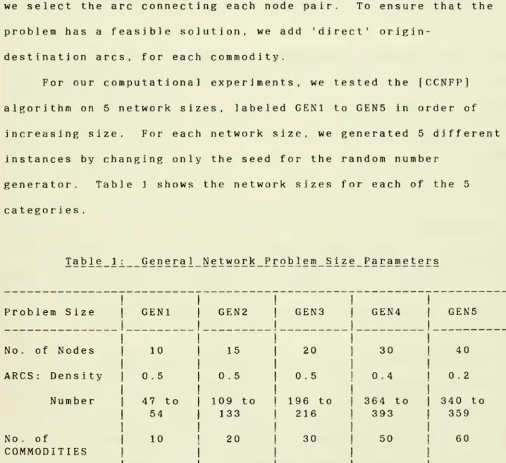
For our computational experiments, we tested the [CCNFP]

algorithm on 5 network sizes, labeled GENl to GENS in order of

increasing size. For each network size, we generated 5 different

instances by changing only the seed for the random number

generator. Table 1 shows the network sizes for each of the 5

categories .

27

For each test problem we set the demand for all commodities

to be the same, say, 1 demand unit. To specify the cost function

for each arc, we first set the number of cost ranges to be four

for all arcs. The widths of each of the 4 cost ranges were chosen so that the optimal solution contains, with high probability,

several arcs that operate in the 'higher' cost ranges in order to

exploit the economies of scale. Table 2 gives the range widths

(in demand units) for the 5 problem categories.

Tabie_22 Range_Widths_X2n_demand_unitsJ^_for_Generai_Networks

1 Range

We assume the fixed cost F. . for the first range in zero for ail

1 J

arcs.

A preprocessing routine executed at the end of the graph

generation procedure identifies, for each commodity k, all arcs

that do not lie on any path from 0(k) to n(k). This procedure

reduces the upper limit of flow (and the number of ranges, if

necessary) on all such arcs.

We coded the composite algorithm in FORTRAN on a PRIME 850

computer. We did not use any special data structures. Djikstra's

[1959] algorithm was used to find shortest paths in the granh. To

initiate the algorithm, we must specify several control

parameters, such as the maximum number of subgradient iterations

to be executed, the intial value of the step size multiplier, and

so on. We now describe these settings below.

(1) The maximum number of subgradient iterations for the

initial run was set at 100. (The subgradient procdure might terminate earlier if either the step size becomes

too small or the Lagrangean subproblem solution is primal feasible.) Subsequent continuation runs of 100

subgradient iterations each were initiated if the gap

between the best Lagrangean lower and the best upper

bound was relatively large and If no significant problem

reduction was achieved In the initial run.

(2) In the first run, the step size multiplier X was

initialized to 2.0. We do not adjust the step size

multiplier during the first 20 iterations or until the

first improvement in z(v) is realized, whichever occurs earlier; thereafter, the step size multiplier was halved

whenever the Lagrangean objective function value did not

improve for 10 consecutive subgradient iterations. In

subsequent runs, \ was initialized to half the initial

value of the previous run (i.e., to 1.0 in the second

run, 0.5 in the third run, and so on). Again, the step

size multiplier was not adjusted during the first 20

iterations or until an improvement in z(v); thereafter,

it was halved after 5 consecutive 'no improvement'

(3) The heuristic procedu

subgradlent iteration

solution obtained fro

is identica] to the i

previous execution of

loca] improvement alg recall that, for each

to D(k) using arcs wi

Lagrangean solution i

for commodity k. Our

procedure if no such

percent of the commod

commodities that cann

algorithm uses the pr

29 re was s . If m the c ni t i a] the he orithm commod th posi s se1ec a1gori path ex it ies ; ot be r evious

initiated once every 10

the initial heuristic

urrent Lagrangean solution

solution derived during the

uristic procedure, then the

is not applied. Also,

ity k, some path from 0(k)

tive flow in the current

ted as the initial routing

thm terminates the heuristic

ists for more than 10

otherwise, for all

outed in this manner, the

initial routing.

(4) After some initial experimentation, we set the

discounting factor for computing the weighted

subgradient equal to 0.2 for all the runs.

Table 3 shows the average, minimum and maximum values of

different performance measures for each of the five problem sizes.

We now interpret some of the key figures. We express all

indicators pertaining to the lower and upper bounding components

of the algorithm as a percentage of the best upper bound that was

obtained .

Qua]_it]^_of_the_fi_nal,_Lagrangean_l_ower_bounds

On average, over all the 25 problem instances, the final lower bound as a percentage of the best upper bound was 98,3 percent. In 4 out of the 25 instances, this gap was zero, while the largest gap was 5.4 percent. As might be expected, this gap seems to be

greater for the larger problems.

Ef£ectl^venes

sof

theLagrangean^basedheur

In all but 4 instances, the Lagrangean-based heuristic improved

upon the initial heuristic solution. On average, the Lagrangean-based heuristic improved the solution by 2.3 percent while the

maximum improvement was 9.0 percent.

Effect

iyenessof

The initial lower bound as a percentage of the best upper bound

was 46.8 percent on average, with a high and low of 58.3 percent

and 39.6 percent respectively. As the problem size increases, the

percentage gap between the initial lower bound and the best upper

31

EfffCtiyeness_of_the_iTiul^t2Bli§£_§^iy5jt!n§Ql-Procedure

The percentage improvement in the Lagrangean lower bound due to

the _Idt_iaj^ascent phase was markedly higher than the improvement

brought about by subsequent multiplier adjustment phases. The

average, minimum and maximum improvements caused by the initial

ascent and subsequent ascent phases are

Initial Ascent Subsequent Ascent Average improvement 22.9 Minimum improvement 13.2 Maximum Improvement 27.7 . 1 0.0 0.3

In 7 out of the 25 problem instances, no improvement was achieved

in the subsequent ascent phases. The percentage improvement due

to Initial ascent does not seem to depend on the problem size.

E§l£2I!D§Q£§_2f_lb?_§ilkgIl§^i£nt_2rocedure

As the problem size increases, more subgradient iterations are

required before the procedure terminates (due to small step size).

As a percentage of the best upper bound, the average, minimum, and

maximum improvements in z(v) are 28.7 percent, 18,8 percent and

35,3 percent, respectively. The subgradient procedure

consistently increased the Lagrangean lower bound by more for the

largest problem size GENS; however, for the other four problem sizes, there is no discernible relationship between this

percentage improvement and the problem size.

lIf?ct2yeness_of_the_2roblem_reducti_on_2I2cedure

The extent to which problems are reduced depends on the absol^ute

Dl^SQitii^? of ^he gap between the Lagrangean lower bound and the

best upper bound, rather than on the percentage gap. On average,

3 _P£§EE2cessing routine eliminated 10.6 percent of the original

kr flow' variables x

1_J

To measure the effectiveness of the

Lagrangean-based problem reduction phase, we use the following

indicator :

PR = 1

-percent of free flow variables at end of algorithm

percent of free flow variables after Preprocessing

This index was 48.5 percent, on average, over all problem

Instances. This procedure fixed al_l the variables for 2 out of

the 25 problem instances, while it did not fix any variable for 1

instance .

Comgutati^onalregui^rements

The figures for CPU times in Table 3 show that the computational

requirements grow very rapidly as the problem size increases.

requir ret ros larger subgra iterat prob] three to tap two ru reduct if we subgra have b subgra Additi sortin at eac and an es m pect pro di en ion ms G time er o ns w ion had d1en een d ien ona1 g ro h St eff

ore time than the other components of the algorithm. In

, this time could have been reduced considerably, if for

blems we had specified a maximum limit of 200 or 300

t iterations in the initial run, rather than the ]00

limit that we used. For almost all the instances of

EN4 and GENS, we had to run the composite algorithm

s before the improvement in the Lagrangean value began

ff . In all these cases, the improvement in the first

as insufficient to lead to any significant problem

and thus, entailed substantial wasted effort. Instead,

allowed the first run to continue for say 200 or 300

t iterations, the total time for problem reduction could

reduced by approximately 2/3rds, and the total time for

t optimization would also have decreased significantly.

savings could have been achieved by employing efficient

utines (required for solving the Lagrangean subproblems

age), special data structures and updating procedures,

icient shortest path subroutine.

THREE-LAYER NETWORKS

This, problem type is a special case of the CCNFP in which (1) nodes of the network are classified into 4 types - Source

nodes. Consolidation points, Breakbulk points, and

Destination nodes,

(2) transshipment is permitted only at consolidation and

breakbulk points, and

(3) the network contains only three categories of arcs:

Source-Consolidation arcs, Conso1 idat ion-Breakbu Ik arcs, and Breakbulk-Destination arcs.

Thus, the origins and destinations are distinct and do not serve

as intermediate nodes. Every commodity must be transported across

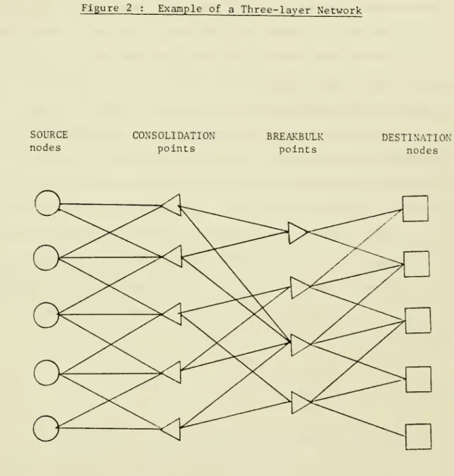
three 'layers' of the network. Figure 2 shows the configuration of a typical network of this type.

33

Figure 2 ; Example of a Three-layer Network

SOURCE nodes CONSOLIDATION points BREAKBULK points DESTINATION nodes

This type of network is of interest as a model for

consolidating and routing LTL shipments, as described at the

outset. Consolidation points are the nodes at which incoming LTL

shipments from the various sources are consolidated into

truckloads before being dispatched to the breakbulk points. At

the breakbulk nodes, incoming truckloads are 'broken', sorted

destination-wise, and forwarded {perhaps as LTL shipments) to

their respective destinations. We permit economies of scale

(i.e., p iecewise- inear concave cost functions) on all arcs of the

network. Note that, although only 3 types of arcs are permitted,

it is possible to model direct source-to-destination links, by

introducing dummy consolidation and breakbulk nodes. This type of

model is very useful when, for operational reasons, the load plan

requires that no shipment is transshipped at more than two

Intermediate points.

To generate the test problems, we specified

(a) the number of source, consolidation, breakbulk, and

destination nodes, denoted as ng, n^, ng, and n^

respectively. The specified number of commodities must

be between Max [ng, np] and ns*n[3 to ensure that each

source and destination node is utilized and that all

commodities have distinct origin-destination pairs; and

(b) the density of the source-conso 1 idat ion ,

consolidation-breakbulk, and breakbu 1k-destinati on arcs, denoted as

•^SC- df;p, and dgp, respectively.

Then, we generated a random network on a 100x100 grid for each

test problem by randomly locating

- _{source nodes in the [0,20]} x [0,100] rectangle,

- _{consolidation and} breakbulk points in the [20,50] x [0,100]

and [50,80] x [0,100] rectangles, respectively, and

35

The selection of the orJgJn-destination pair for each commodity

was random, except for modifications to ensure that all source and

destination nodes are used and that no origin-destination pair is

assigned to more than one commodity. To generate the arcs for the

network, we identified for each source node the (dg^nQ) closest

consolidation points and included the corresponding

source-consolidation arcs in the network. Similarly, each destination

node is connected to the (dp^nR) closest breakbulk points. This

choice reflects the characteristic of practical problems in which

each source and destination is typically connected to a few of the

closest transshipment (consolidation and/or breakbulk) points.

The consolidation-breakbulk arcs are chosen randomly with

probability

d^B-For each commodity, it is necessary to check if the current

graph has at least one path from the commodity's origin to its

destination, in order to ensure that the problem is feasible. If

some commodity k does not have any path from 0(k) to D(k) , an

appropriate consolidation-breakbulk arc is randomly added to

ensure feasibility.

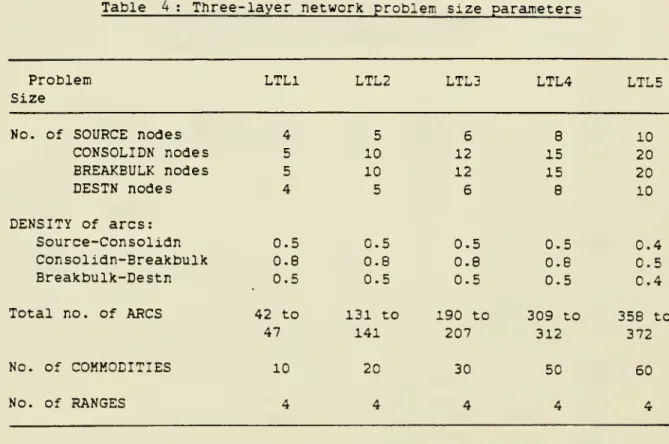
For our computational experiments, we generated problems in 5

different sizes, labeled LTLl to LTL5, for each of which we

generated 5 problem instances. Table 4 specifies the problem

sizes for each category.

All other problem parameters - for the demand, variable cost

structure, and range widths - were identical to those used for

generating the general CCNFP test problems.

modifications for exploiting the special LTL structure, to solve

the 25 test instances of the three-layer problem. All the

solution parameters in the CCNFP algorithm, e.g. the maximum

number of subgradient iterations per run, had the same values used

for solving general networks.

Table 5 presents the summary statistics for the five problem

sizes. As before, we consider the performance of each component

of the composite procedure in turn. All the improvements in the

upper and lower bounds are evaluated in terms of percentages of

the best final upper bound.

Qual^_ity_of_the_fi,na2_L§gI§DS?§Il_i2wer_bound

The average value of the final lower bound as a percentage of the

best upper bound was 99.6 percent while the largest gap was 2.5

percent. In 19 out of the 25 problem instances, there was no gap

between the final lower bound and the best upper bound, indicating

that the optimal solution had been found in all these cases.

l££§cti^yeness_of_the_Lagrangean-based_heuristj^c_procedure

In all but 3 instances, the Lagrangean-based heuristic improved upon the intlal heuristic solution. As a percentage of the best

upper bound, the Lagrangean-based heuristic improved the initial

solution by an average of 6.8 percent; the maximum improvement was

24.8 percent .

l£f§£liy§0§s

sof

The average, minimum, and maximum values of the initial lower

bound as a percentage of the best upper bound were 89.6 percent,

83.8 percent, and 95.4 percent respectively. For this class of

problems, therefore, the multiplier initialization method seems to

37

Table 4 ; Three-layer network problem size para^ieters

Problem Size

LTLl LTL2 LTL3 LTL4 LTL5

TABLE 5

Summary statistics for test runs on Three-layer Network problems

Problem class LTLl LTL2 LTL3 LTL4 LTL4 SITE

39

IIf§£liHeness_of_the_multi22ier_adjustment_method

As before, the initial ascent phase gives significantly better

improvements to the Lagrangean lower bound than the subsequent

multiplier adjustment phases. The average, minimum, and maximum

values of the improvement in the lower bound as a percentage of

the best upper bound are

Average increase Minimum increase Maximum increase Initial Ascent 4 . 45 1.11 7 . 73 Subsequent

COMPARISON OF RESULTS FOR GENERAL AND THREE-LAYER PROBLEMS

The three-layer problems that we tested were obviously easier

to solve using our algorithm than the general network problems.

The performance of every component of the algorithm was superior

for the three-layer problems. First, the preprocessing routine

was significantly more effective for these problems (75.7 percent

reduction compared to 10.6 percent for general networks). Because

of the significant reduction in problem size at the preprocessing

stage, the initial lower bound was on average 89.6 percent of the

best upper bound, as compared to only 46.8 percent for general problems. Since the percentage gap between the lower and upper

bound is relatively small from the beginning, the ascent and

subgradient phases did not improve the bounds as much for three

layer problems as for general network problems. Also, since the

gaps were smaller, more reduction was possible, and the

three-layer problems required fewer iterations (and hence less CPU

time). Finally, the Lagrangean-based heuristic procedure also

performed better for this class of problems (improving the initial

heuristic solution by 6.8 percent compared to 2.3 percent). Since

the final set of Lagrange multipliers were closer to the optimal values, the Lagrangean-based initial solutions might have been

better than for general network problems. Thus, the effectiveness

of each component of the composite algorithm contributes to

41

CONCLyDING_REMARKS

In this paper we developed a composite procedure for finding

good upper and lower bounds for a special case of a network design

problem that Is of considerable practical importance. By

combining a mu1t_i p1 ier-adjustment procedure with a subgradient

procedure, a problem reduction phase, and a Lagrangean-based

heuristic algorithm, we were able to solve fairly large

concave-cost network flow problems. This composite algorithm exploits the

special structure of the CCNFP, and the computational results

confirm the usefulness of a strategy that combines lower and upper

bounding schemes, which are based on the partial optimization of

some related problems. Also, the performance of such algorithms

seems to improve substantially when the networks have certain

special structures. See Balakrishnan (1985) for more details on

the algorithm and on the computational experiments. Balakrishnan

(1985) also explores several possible extensions to the algorithm;

in particular, he considers the use of a more complex subproblem

in the Lagrangean, and the development of an ascent procedure that

permits Zjj(v) to change.

ACKNOWLEDGEMENT

This research was supported by a grant from the Center for

Transportation Studies, Massachusetts Institute of Technology,

Cambridge , MA .

BALAKRISHNAN , A. 1984. Va]_id_Inegua1 i ti es_and_AIgori thms_for_the

Network_Design_Prob2em_wi_th_an_Agglicati^on_to_LTL Conso^idatj^on . Doctoral dissertation, Sloan School of

Management, Massachusetts Institute of Technology, Cambridge,

MA . , December .

CROWDER, H. 1976. "Computational Improvements for Subgradient Optimization", S^mpos i_a_Mathemati^ca , Vol. 19, pp. 357-372.

DIJKSTRA, E. W. 1959. "A Note on Two Problems in Connexion with Graphs", Numer

scheMa

ERICKSON, R. E.. C. L. MONMA and A. P. VEINOTT. 1981. "Minimum

Concave-cost Network Flows", Working paper.

FLORIAN, M., and M. KLEIN. 1971. "Deterministic Production Planning With Concave Costs and Capacity Constraints", Management_Sclence, Vol. 18, pp. 12-20.

PONG, C. 0. and M. R. RAO. 1975. "Capacity Expansion with Two

Producing Regions and Concave Costs", Management_Sc ence , Vol.

22, No. 3, pp. 331-339, November.

GALLO, G., and C. SODINI. 1979. "Concave Cost Minimization on

Networks", Eurogean_Jou

rnalof

pp . 239-249

GEOFFRION, A. M. 1974. "Lagrangian Relaxation for Integer

Programming", MathematicaX_Programmi^ng_Stud^_2 , pp. 82-114.

LAMAR, B. 1983. "Les -Than-Truck oad Freight Consolidation and

Routing Strategies: A Mathematical Programming Procedure",

Project Report No. CTS/IU-83.2, Center for Transportation

Studi es , M. I . T

LAMAR, B., Y. SHEFFI and W. POWELL. 1984. "Bounding Procedures for

Fixed Charge, Multicommodity Network Design Problems", Working Paper , December .

LOVE, S. F. 1973. "Bound Production and Inventory Models with

Piecewise Linear Concave Costs", Management_Science , Vol. 20. pp . 313-318

LUSS, H. 1979. "A Capac1 ty-Expansion Model for Two Facility

Types",

NavalResearchLogi

csQuar

291-303.

POWELL, W. 1985. "A Local Improvement Heuristic for the Design of

Less-Than-Truckload Motor Carrier Networks", Princeton

43

POWELL. W. B.. and Y. SHEFFI. 1983. "The Load Planning Problem of

LTL Motor Carriers: Problem Description and a Proposed

Solution Approach", Transgortat_i

onRes

380.

SOLAND , R, M. 1974. "Optimal Facility Location with Concave

Costs", Operations_Research , Vol. 22, pp. 373-382.

SWOVELAND, C. 1975. "A Deterministic Multi-Period Production

Planning Model with Piecewise Concave Production and

Holding-Backorder Costs",

ManagementSc

TAHA , H. A. 1973. "Concave Minimization over a Convex Polyhedron"

Nava1 Legist

icsResearchQuar

ZADEH, N. 1973. "On Building Minimum Cost Communication Networks"

Networks, Vol. 3, No. 4, pp. 315-331.

ZADEH, N. 1974. "On Building Minimum Cost Communication Networks Over Time". Networks, Vol. 4, No. 1, pp. 19-34.

ZANGWILL, W. I. 1968. "Minimum Concave Cost Flows in Certain Networks", Management_Science , Vol. 14, No. 7. pp. 429-450.

MIT LIBRARIES

DatB

m^i^M