MIT Joint Program on the
Science and Policy of Global Change
A Comparison of the Behavior of AOGCMs in
Transient Climate Change Experiments
Andrei P. Sokolov, Chris E. Forest and Peter H. Stone
Report No. 81 December 2001
The MIT Joint Program on the Science and Policy of Global Change is an organization for research, independent policy analysis, and public education in global environmental change. It seeks to provide leadership in understanding scientific, economic, and ecological aspects of this difficult issue, and combining them into policy assessments that serve the needs of ongoing national and international discussions. To this end, the Program brings together an interdisciplinary group from two established research centers at MIT: the Center for Global Change Science (CGCS) and the Center for Energy and Environmental Policy Research (CEEPR). These two centers bridge many key areas of the needed intellectual work, and additional essential areas are covered by other MIT departments, by collaboration with the Ecosystems Center of the Marine Biology Laboratory (MBL) at Woods Hole, and by short- and long-term visitors to the Program. The Program involves sponsorship and active participation by industry, government, and non-profit organizations.
To inform processes of policy development and implementation, climate change research needs to focus on improving the prediction of those variables that are most relevant to economic, social, and environmental effects. In turn, the greenhouse gas and atmospheric aerosol assumptions underlying climate analysis need to be related to the economic, technological, and political forces that drive emissions, and to the results of international agreements and mitigation. Further, assessments of possible societal and ecosystem impacts, and analysis of mitigation strategies, need to be based on realistic evaluation of the uncertainties of climate science.
This report is one of a series intended to communicate research results and improve public understanding of climate issues, thereby contributing to informed debate about the climate issue, the uncertainties, and the economic and social implications of policy alternatives. Titles in the Report Series to date are listed on the inside back cover. Henry D. Jacoby and Ronald G. Prinn,
Program Co-Directors
For more information, please contact the Joint Program Office
Postal Address: Joint Program on the Science and Policy of Global Change MIT E40-271
77 Massachusetts Avenue
Cambridge MA 02139-4307 (USA) Location: One Amherst Street, Cambridge
Building E40, Room 271
Massachusetts Institute of Technology Access: Phone: (617) 253-7492
Fax: (617) 253-9845
E-mail: g l o ba l ch a n g e @ m i t .e d u
Web site: h t t p:/ / m i t .e d u / g l o ba l ch a n g e /
A Comparison of the Behavior of Different AOGCMs in Transient Climate Change Experiments
Andrei P. Sokolov, Chris E. Forest and Peter H. Stone Abstract
The transient response of both surface air temperature and deep ocean temperature to an increasing external forcing strongly depends on climate sensitivity and the rate of the heat mixing into the deep ocean, estimates for both of which have large uncertainty. In this paper we describe a method for estimating rates of oceanic heat uptake for coupled atmosphere/ocean general circulation models from results of transient climate change simulations. For models considered in this study, the estimates vary more than threefold. Nevertheless, values for all models fall in the 5–95% interval of the range implied by the climate record for the last century.
The MIT 2D climate model, with an appropriate choice of parameters, matches changes in surface air temperature and sea level rise simulated by different models. It also reproduces the overall range of changes in precipitation.
Contents
1. Introduction ... 1
2. Model Description... 2
3. Estimating Rates of Heat Uptake for Different AOGCMs... 3
4. Change in Precipitation... 10
5. Conclusions ... 12
References ... 12
1. INTRODUCTION
At the present time, coupled atmosphere-ocean general circulation models (AOGCMs) are widely used for making projections of possible future climate change. However, results produced by different AOGCMs differ significantly even for similar changes in external forcing.
For example, in simulations with 1% per year increase in CO2 concentration, performed in the framework of the Coupled Models Intercomparison Project (http://www-pcmdi.llnl.gov/cmip/ index.html), the increase in surface air temperature (SAT) at the time of CO2 doubling
(an average for years 61–80) simulated by different models ranges from 1.32 o
C to 2.15 o C (Covey et al., 2000).
The transient response produced by a given model is, to a large part, determined by two characteristics of the model: sensitivity to an external forcing and the rate of heat uptake by the ocean. While sensitivities for many AOGCMs are known and given in the literature, differences in the rates of oceanic heat uptake are not well estimated. The ratio of the SAT increase at the time of CO2 doubling to the equilibrium model sensitivity, which is often used to compare transient responses of different AOGCMs (see for example, Murphy and Mitchell, 1995), depends on both the rate of oceanic heat uptake and model sensitivity. In upwelling-diffusion models, a number of parameters, such as a mixed layer depth, the upwelling rate, a diffusion coefficient and so on, are varied to fit the behavior of different AOGCMs (Wigley and Raper,
1993; Cubasch et al., 2001). The use of multiple parameters makes it difficult to compare the rates of heat uptake by different models. In this study, we obtain quantitative estimates for the oceanic heat uptake by choosing parameters of the MIT 2D climate model to match behavior of different AOGCMs. Then, the effective heat diffusivity of the MIT model provides a measure of the rate of the heat uptake by the deep ocean for those models. This study was conducted as a part of subproject #20 of CMIP2.
2. MODEL DESCRIPTION
The atmospheric component of the MIT 2D climate model (Sokolov and Stone, 1998) is a zonal averaged statistical-dynamical model developed from the GISS AGCM (Hansen et al., 1883). It includes parameterizations of all the main physical processes in the atmosphere and therefore, can reproduce major feedbacks. It also includes parameterizations for atmospheric heat,
moisture, and momentum transports by large-scale eddies (Stone and Yao, 1987, 1990). For any given AOGCM, model sensitivity, as well as the rate of the oceanic heat uptake, depend on how different feedbacks are depicted by the model, which, in turn, is defined by a large number of factors, such as parameterizations of different physical processes, horizontal and vertical resolutions, and so on. In contrast, the sensitivity (S) of the MIT 2D model can be specified by changing the strength of the cloud feedback. Namely, the amount of clouds used in radiative transfer calculations is defined as C = Co(1+k∆Ts), where Co is the simulated cloud cover and
∆Ts is the deviation of global mean SAT from its value in an equilibrium present-day climate simulation (Hansen et al., 1993). It was shown by Sokolov and Stone (1998) that the dependence of changes in different climate variables, such as precipitation, surface fluxes and so on, on climate sensitivity shown by the MIT model is similar to the dependence found in equilibrium climate change simulations with different AGCMs.
The ocean component of the MIT 2D climate model consists of a Q-flux mixed layer model with a deep ocean diffusive model beneath it. The mixed layer depth is prescribed from
observations as a function of season and latitude. In addition to the temperature of the mixed layer, the model also calculates the averaged temperature of the seasonal thermocline and the temperature at the annual maximum depth of the mixed layer (Russell et al., 1985). In contrast with conventional diffusive models, diffusion in the MIT model is not applied to temperature itself but to the temperature difference from its values in a present-day climate simulation (Hansen et al., 1984; Sokolov and Stone, 1998). In our model, diffusion represents a cumulative effect of the mixing of heat by all physical processes and therefore, the values of the diffusion coefficients are significantly larger than those used in sub-grid scale diffusion parameterizations in OGCMs. The values of effective diffusion coefficients calculated from data on tritium mixing into deep ocean (Hansen et al., 1984) vary from 0.2 cm2
/s in tropics to about 10 cm2
/s in high latitudes with a global averaged value of 2.5 cm2/s. The rate of heat penetration into the deep ocean is varied by multiplying diffusion coefficients by the same factor at each latitude thereby preserving the spatial structure of the heat uptake. Despite the ocean component’s simplicity, the MIT model can reproduce the evolution of different AOGCMs in typical climate change scenarios for about 100–150 years, in terms of global mean SAT and the sea level rise due to thermal expansion of the deep ocean (Sokolov and Stone, 1998).
3. ESTIMATING RATES OF HEAT UPTAKE FOR DIFFERENT AOGCMS
A number of climate change simulations with different coupled AOGCMs have been carried out in the second stage of the Coupled Model Intercomparison Project (CMIP2) (http://www-pcmdi. llnl.gov/cmip/index.html). In these simulations, models were forced by 1% per year increase in the atmospheric CO2 concentration for 80 years. To compare behavior of different AOGCMs, we obtain versions of the MIT 2D climate model that fit the response of the models in question. The global averaged values of diffusion coefficients (Kv) used in the fits for different AOGCMs give a measure for their rate of oceanic heat uptake.
Apart from the region of low climate sensitivity (S < 1 oC), SAT change and sea level rise due to thermal expansion of the ocean are unequivocally defined by S and Kv (Figure 1). Thus, a fit for a given AOGCM can be estimated based on the data on surface warming and thermal expansion of the ocean. However, if the value of the model’s sensitivity is already known, then the value of Kv can be chosen so that the transient change of SAT for this model is reproduced by the MIT 2D model with the same sensitivity. Data on sea level rise then can be used to check the quality of the fit. We used the latter approach whenever possible.
0 2 4 6 8 0 1 2 3 4 5 Sensitivity ( S ) 0.50 0.50 0.50 1.00 1.00 1.50 2.00 2.00 2.50 3.0 0 3.50 2.50 2.50 5.00 7.50 7.50 12.50 12.50 15.00 15.00 GISS-GR GFDL-R15 CGCM1 MRI1 PCM ECHAM3 GFDL Kv 10.00 7.50 5.00 1.50 NCAR CSM ECHAM3/LSG HadCM2 HadCM3 CSIRO CSIRO 10.0 0 GISS-SB
Figure 1. Changes in surface air temperature and sea level rise due to thermal expansion of the ocean at
Sensitivity for a given AOGCM is usually defined as the equilibrium surface warming (∆Teq) simulated by the corresponding atmospheric model coupled to a mixed layer ocean model in response to the doubling of atmospheric CO2 concentration. It varies from about 2
o
C to about 5 oC among existing AOGCMs (Cubasch et al., 2001). The estimates for an equilibrium
sensitivity from simulations with coupled AOGCMs are available to date only for the HadCM2 (Senior and Mitchel, 2000) and the GFDL_R15 (Stouffer and Manabe, 1999) models. In both cases they are somewhat different from those obtained in the simulations with mixed layer ocean models.
It was noticed by Murphy (1995) that the sensitivity of a coupled AOGCM changes with time due to changes in the strength of different atmospheric feedbacks.1 The energy balance of the climate system can be described by the following simple equation:
) ( ) ( ) ( t T t F t t T C = − ∆ ∂ ∆ ∂ λ , (1)
where C is the heat capacity of the system, F(t) is an external forcing, ∆T is the change in surface
temperature and λ is a feedback parameter. In equilibrium, λeq= F2xCO2/∆Teq, where F2xCO2 is a forcing due to CO2 doubling. In a transient run, a time-dependent effective feedback parameter can be estimated as follows:
) ( ) ( ) ( ) ( t T t R t F t toa eff ∆ − = λ , (2)
where Rtoa(t) is the net radiative flux at the top of the atmosphere. An effective climate
sensitivity, ∆Teff, is then defined as what the equilibrium surface warming due to CO2 doubling would be if λ = λeff, ∆Teff = F2xCO2/λeff. The values of the effective sensitivity at the time of CO2 doubling for some AOGCMs used in the CMIP2 simulations are given in Cubasch et al. (2001) and are shown in Table 1. As can be seen, the effective sensitivity at the time of CO2 doubling is usually smaller than ∆Teq, and for some models significantly smaller.
Table 1. Values of equilibrium and effective climate sensitivities at the time of CO2
doubling from Cubasch et al. (2001). Values of ∆Teq are from simulations with
mixed-layer ocean models, while ∆Teff are from transient simulations with coupled AOGCMs.
Model ∆∆∆∆Teq ∆∆∆∆Teff at 2xCO2
CGCM1 3.5 3.6 CSIRO 4.3 3.7 ECHAM3/LSG 2.5 2.2 GFDL_R15 3.7 4.2 HadCM2 4.1 2.5 HadCM3 3.3 3.0 MRI1 4.8 2.6 NCAR_CSM 2.1 1.9 1
Changes in the model sensitivity described by Senior and Mitchell (2000) occurring after a few hundreds years of integration and associated with changes in the deep ocean circulation are not relevant when results of relatively short-term simulations are analyzed.
Satisfactory fits have been obtained for a number of the AOGCMs using equilibrium climate sensitivities (Sokolov and Stone, 1998). However, for some models used in CMIP2 simulations, thermal expansion was overestimated by the versions of the MIT model with S equal to the model’s equilibrium climate sensitivity, even so, they fit the SAT changes. For example, very large effective diffusion coefficients (Kv = 500 cm
2
/s) are required to reproduce changes in SAT simulated by the MRI1 AOGCM (Figure 2a) when the model’s equilibrium climate sensitivity of 4.8 oC is used. However, the MIT climate model with these parameters produces a
significantly larger sea level rise (Fig. 2b).2 At the same time, the MIT model with S = 2.6 oC and Kv = 50 cm2/s reproduces changes in both SAT and sea level.
0 20 40 60 80 100 0.0 0.5 1.0 1.5 2.0 2.5 3.0 3.5 Degree Centigrade 20 40 60 80 100 0.0 5.0 10.0 15.0 20.0 25.0 30.0 cm * * * * 0 20 40 60 80 100
Years from start of simulation 0.0 0.5 1.0 1.5 2.0 2.5 3.0 3.5 Degree Centigrade 20 40 60 80 100
Years from start of simulation 0.0 5.0 10.0 15.0 20.0 25.0 30.0 cm * * * * a) b) c) d)
Figure 2. Changes of annual mean global mean surface air temperature and sea level (thermal expansion)
in simulations with the MRI1 (a,b) and ECHAM3/LSG (c,d) AOGCMs and in simulations with the versions of the MIT 2D Climate Model with effective (solid lines) and equilibrium (dashed lines) climate sensitivities. Data from CMIP2 simulations with AOGCMs are shown by dashed-dotted line (SAT) and by * (sea level).
2 Unfortunately, while changes in SAT from these simulations are available on an annual basis, sea level rise due to
thermal expansion of the ocean is not. The data required to calculate thermal expansion were saved as a 20 year mean for four consecutive segments of the simulations. In this study we used data on sea level rise for these four periods provided by Sarah Raper (Raper et al., 2001).
Using the effective sensitivity, instead of an equilibrium one, leads to significantly better simulation of the oceanic thermal expansion not only for the MRI1 but also for the
ECHAM3/LSG AOGCM in spite of the small difference between the two sensitivities for the latter model. On the other hand, fits with effective and equilibrium sensitivities give very close results for the CSIRO and GFDL_R15 models (Figure 3). Positions of the final fits for different AOGCMs using S = ∆Teff are shown in Figure 1 by filled circles. Positions of the versions of the MIT model which reproduce changes in SAT for ECHAM3/LSG, CSIRO and GFDL_R15 using their equilibrium sensitivities are shown by open circles. Due to the weak dependence of changes in SAT on Kv for low climate sensitivities, the two fits for the ECHAM3/LSG model have
significantly different rates of oceanic uptake. Sea level rise, on the contrary, is rather sensitive to changes in Kv in this region of parameter space. This, together with the relatively small increase in sea level projected by the ECHAM3/LSG model explains the noticeable difference between this model’s fits with equilibrium and effective sensitivities. The opposite is true for both the CSIRO and the GFDL_R15 models. It should be noted that the difference in sea level rise projections by fits with different sensitivities increases with time. In general, the use of an effective sensitivity instead of an equilibrium one leads to better simulation of sea level rise.
0 20 40 60 80 100 0.0 0.5 1.0 1.5 2.0 2.5 3.0 3.5 Degree Centigrade 20 40 60 80 100 0.0 5.0 10.0 15.0 20.0 25.0 30.0 cm * * * * 0 20 40 60 80 100
Years from start of simulation 0.0 0.5 1.0 1.5 2.0 2.5 3.0 3.5 Degree Centigrade 20 40 60 80 100
Years from start of simulation 0.0 5.0 10.0 15.0 20.0 25.0 30.0 cm * * * * a) b) c) d)
Table 2. Adjusted radiative forcing due to CO2 doubling for different models. Model Forcing (W/m2) CSIRO 3.45 HadCM2 3.47 HadCM3 3.74 NCAR_CSM 3.60 PCM 3.60
GISS and MIT 2D 3.84
In all simulations discussed above, the MIT climate model was forced by radiative forcing calculated by its radiation scheme (in contrast with energy balance models where the radiative forcing is prescribed). It has been shown, however, that different models produce different forcings for the same increase in the CO2 concentration (Cess et al., 1993). The values of the adjusted radiative forcing3
due to CO2 doubling for some models are given in Table 2. A number of additional simulations have been carried out to evaluate the impact of these differences. The differences in forcing were taken into account in the following way. As is well known, radiative forcing increases linearly with an exponential increase in CO2, namely
F(t) = καt, where α is a rate of CO2 increase and κ is a coefficient different for different models. A value of κ for a given model is defined by the details of its radiation code (for the MIT 2D
model κ = 5.35) and cannot be changed. Therefore, we changed α such that the forcing averaged
over years 61–80 matched a given model’s value. However, if differences in forcing are taken into account, the 2D model’s sensitivity (S) must also be changed to match the “specific” sensitivity, that is an equilibrium SAT increase due to forcing of 1 W/m2, of a given. The values of S used in simulations with 1% per year increase in CO2 (Table 1, 2
nd
column) are defined as a surface warming in response to CO2 doubling or, more exactly, to the forcing produced by CO2 doubling in the MIT model (that is, 3.84 W/m2
). For example, S = 3.7 o
C, matching the
equilibrium sensitivity of the CSIRO AOGCM, corresponds to a warming of 0.96 oC/(W/m2) for the MIT 2D model while “specific” sensitivity of the CSIRO AOGCM is 1.07 o
C/(W/m2 ). Therefore, a climate sensitivity of 4.12 oC should be used in the simulation with the MIT 2D model to match a “specific” sensitivity of the CSIRO AOGCM.
The CSIRO and HadCM2 AOGCMs produce forcing most different from that of the 2D model (Table 2). However, simulations with corrected values of forcings and sensitivities even for these models (Figure 4) show small differences compared to the simulations with the original sensitivities and forcing. Such a small impact of different forcing on the results of simulations with increasing CO2 can be explained through simple analysis of equation (1). For linear forcing, equation (1) has an analytical solution under the assumption that C is fixed. Namely:
)) 1 ( ( ) ( γ τ τ t s t S t e T = − − − ∆ , (3) where γ =κα , −1 =λ S and τ =SC. 3
Adjusted refers to the radiative imbalance at the tropopause after the stratospheric temperatures have adjusted to the new CO2 concentration. This adjusted forcing must be used in energy balance models (EBMs) to reproduce the
0 20 40 60 80 100 0.0 0.5 1.0 1.5 2.0 2.5 3.0 3.5 Degree Centigrade 20 40 60 80 100 0.0 5.0 10.0 15.0 20.0 25.0 30.0 cm * * * * 0 20 40 60 80 100
Years from start of simulation 0.0 0.5 1.0 1.5 2.0 2.5 3.0 3.5 Degree Centigrade 20 40 60 80 100
Years from start of simulation 0.0 5.0 10.0 15.0 20.0 25.0 30.0 cm * * * * a) b) c) d)
Figure 4. Changes of annual mean global mean surface air temperature and sea level (thermal expansion)
in simulations with the CSIRO (a,b) and HadCM2 (c,d) AOGCMs and in simulations with the versions of the MIT 2D Climate Model with corrected (dashed lines) and uncorrected (solid lines) forcing. Data from CMIP2 simulations with AOGCMs are shown by dashed-dotted line (SAT) and by * (sea level). Data from CMIP2 simulation with AOGCMs are shown by dashed-dotted line (SAT) and by * (sea level).
However, for equation (1) to be a correct equation for the change in surface air temperature, C should be the heat capacity of the part of the deep ocean affected by warming at a time t but not the heat capacity of the whole ocean. The former is proportional to the depth of heat anomaly penetration, which for a diffusive model is proportional to Kv *t (Hansen et al., 1985). While equation (3) is not an exact solution of equation (1) for time dependent C, it approximates a numerical solution of equation (1) rather well with τ proportional to S Kv *t . While values of γ and S are different in simulations with corrected and uncorrected forcings, their product is the same in both cases. As a result, the difference in ∆Ts is relatively small in spite of difference in τ. As could be expected, the difference is large for the CSIRO AOGCM due to a larger τ.
Analogous simulations with other models have shown that taking into account differences in forcing between different AOGCMs does not noticeably affect estimates of the rates of oceanic heat uptake. Because data on radiative forcing are not available for all models, the estimates from simulations with 1% per year increase in CO2 concentration were used. Fits for the
GISS_GR (Russell et al., 1995) and the GISS_SB (Sun and Bleck, 2001) AOGCMs were obtained based on the data on SAT and thermal expansion, provided by the models’ authors, without prior knowledge of the models’ sensitivities. Fits for some models used in CMIP2 simulations were not obtained due to absence of data on sea level rise.
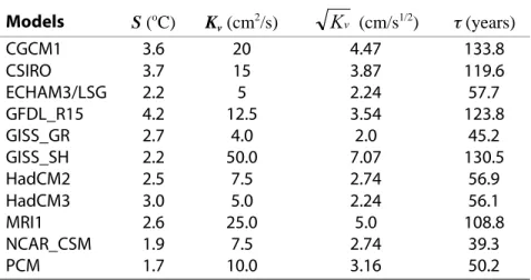
As follows from above, the most natural measure for the rate of oceanic heat uptake for the MIT 2D model is Kv. For models given in Table 3, Kv varies from 2.0 to 7.1 cm/s1/2.
In Figure 5 a probability density function (PDF) for Kv calculated from data for models is
compared with the one based on comparison with observations (Forest et al., 2001). The PDF for models was obtained by fitting β distributions to data from Table 3. Data for all models were
weighted equally. Though shapes of the two PDFs are different, values of Kv for all models fall into the 5–95% interval suggested by observations. The means/medians of the two distributions are also not very different, 3.49/3.33 cm/s1/2 and 4.20/4.40 cm/s1/2 for models and observations, respectively. It should be noted that, because the observations do not place an upper bound on Kv, a subjective bound of Kv = 64 cm
2
/s was imposed. For a different choice of an upper bound the values of fractals would be somewhat deferent. A PDF for the rate of oceanic heat uptake, which is a key factor for projecting future climate change, based on estimates derived from comparison with both observations and different AOGCMs was used by Webster et al. (2001).
Marginal PDF : Effective Ocean Diffusivity
0 1 4 9 16 25 36 49 64
Effective ocean diffusivity [cm2/s] 0.00 0.10 0.20 0.30 0.40 Density Observations Models
Figure 5. Probability density functions for the rate of oceanic heat uptake from models (dashed) and
observations (solid). The whisker plots show the 2.5–97.5% (dots), 5–95% (vertical bars on ends), and 25–75% (box) probability ranges along with the median (bar within box) and mean (diamond) for each distribution.
Table 3. Parameters of the versions of the MIT climate model simulating
behavior of different AOGCMs. The values of τ are at the time of CO2 doubling.
Parameters of corresponding versions of the 2D model
Models S (oC) K v (cm2/s) Kv (cm/s1/2) τ (years) CGCM1 3.6 20 4.47 133.8 CSIRO 3.7 15 3.87 119.6 ECHAM3/LSG 2.2 5 2.24 57.7 GFDL_R15 4.2 12.5 3.54 123.8 GISS_GR 2.7 4.0 2.0 45.2 GISS_SH 2.2 50.0 7.07 130.5 HadCM2 2.5 7.5 2.74 56.9 HadCM3 3.0 5.0 2.24 56.1 MRI1 2.6 25.0 5.0 108.8 NCAR_CSM 1.9 7.5 2.74 39.3 PCM 1.7 10.0 3.16 50.2 4. CHANGE IN PRECIPITATION
As shown above, the MIT 2D climate model with an appropriate choice of climate sensitivity and an effective diffusion coefficient can reproduce changes in SAT and sea level projected by different AOGCMs. Because the MIT climate model is used as a component of the MIT
Integrated Global System Model (IGSM) (Prinn et al., 1999), it is also important to know how it simulates transient changes in other climate variables. Precipitation is of particular interest because it is used as an input by both the Terrestrial Ecosystem Model (Xiao et al., 1997) and the Natural Emission Model (Liu, 1997), which are included in the IGSM
Changes in precipitation, even on a global scale, are not unequivocally defined by global characteristics of a given model, but depend on details of the physical parameterizations.
Thereby, a version of the MIT model matching transient changes in SAT and sea level simulated by a particular AOGCM does not necessarily reproduce changes in precipitation for the same model. For example, the MIT model simulates rather well changes in precipitation for the CSIRO and ECHAM3/LSG AOGCMs (Figure 6a), but significantly overestimates the increase in precipitation for the CGCM1 model and underestimates it for the MRI1 model (Figure 6b). Figures 7 reveals a strong positive correlation between changes in precipitation and SAT in different simulations with the MIT climate model. In contrast, a noticeably weaker correlation exists between changes in those two variables as simulated by different AOGCMs. While the results of simulations with the MIT model almost fall on a straight line, the results from
AOGCMs are more scattered. Covey et al. (2000) showed that the correlation is also weak when results of all CMIP2 simulations are compared. While precipitation increases (in terms of the global average) with an increase in SAT in all simulations, the rate of such an increase for a given model is mainly defined by parameterizations of different physical processes, such as convection, cloud formation, or calculation of surface fluxes (Washington and Meehl, 1993). Because the only difference between different versions of the MIT model is the strength of cloud
feedback, the above-mentioned strong correlation between changes in SAT and precipitation for the MIT model simulations is not surprising. As a result, the MIT climate model cannot simulate some particular climate change regimes, such as cold and wet or hot and dry climates.
Nevertheless, it reproduces the range of increases in precipitation produced by AOGCMs.
0 20 40 60 80 100 Years from start of simulation 0
2 4 6 a)
0 20 40 60 80 100 Years from start of simulation 0
2 4 6 b)
Percentage Change (%) Percentage Change (%)
Figure 6. Changes of annual mean global mean precipitation in simulations with AOGCMs (thick lines)
and with the matching versions of the MIT 2D Climate Model (thin lines); a) for CSIRO (dashed lines) and ECHAM3 (solid) models, b) for MRI (dashed) and CGCM1 (solid) models.
0 1 2 3 4 5 6 Change in Precipitation (%) Surface warming (˚C) 0 0.5 1 1.5 2 2.5 3
Figure 7. Percentage change in globally and annually averaged precipitation as a function of global mean
warming at the time of doubling of CO2 as produced by different AOGCMs (triangles) from
5. CONCLUSIONS
The MIT 2D climate model with an appropriate choice of parameters defining the model’s sensitivity and the rate of oceanic heat uptake can successfully reproduce both an increase in surface air temperature and sea level rise due to thermal expansion of the deep ocean projected by a given AOGCM. The rate of heat uptake by the deep ocean in the MIT model is defined by one parameter, namely the global averaged value of an effective diffusion coefficient. This provides quantitative estimates of the strength of oceanic heat uptake for different AOGCMs.
Use of an effective climate sensitivity at the time of CO2 doubling, instead of an equilibrium sensitivity, leads to better fits and for some models to significantly different estimates of oceanic heat uptake. At the same time, taking into account differences in the radiative forcing between different AOGCMs does not noticeably affect those estimates.
Estimated values of effective diffusion coefficients for AOGCMs considered in this study differ by more than factor of three (in terms of Kv), and this introduces considerable
uncertainty in long-term projections of climate change. It should be noted that the values for all models fall within the 5–95% interval of the range derived from comparisons with the 20th century climate record (Forest et al., 2001).
Different versions of the MIT climate model show stronger correlation between changes in SAT and global averaged precipitation than simulated by AOGCMs. Nevertheless, the MIT climate model, while not matching results of some models, does capture the range of increases in precipitation produced by AOGCMs.
Acknowledgments. We thank Sarah Raper for providing us with data on sea level rise for CMIP2
simulations and Gary Russell and Shan Sun for the date for GISS_GR and GISS_SB models. We also thank PCMDI and CMIP2 participants for making CMIP2 data available.
REFERENCES
Cess, R.D., et al., 1993: Uncertainties in Carbon Dioxide Radiative Forcing in Atmospheric General Circulation Models. Science, 262: 1251-1255.
Covey, C., K.M. AchutaRao, S.J. Lambert and K.E. Taylor, 2000: Intercomparison of Present and Future Climates Simulated by Coupled Ocean-Atmosphere GCMs, PCMDI Report #66, 52pp.
Cubasch, U., et al., 2001: Projection of Future Climate Change. In: Climate Change 2001. The Scientific Basis. J.T. Houghton et al. (eds.), Cambridge University Press, Cambridge. Forest, C.E., et al., 2001: Quantifying Uncertainties in Climate System Properties Using Recent
Climate Observations. Science, in press.
Hansen, J., et al., 1983: Efficient Three Dimensional Global Models for Climate Studies: Models I and II. Mon. Wea. Rev., 111: 609-662.
Hansen, J., et al., 1984: Climate Sensitivity: Analysis of Feedback Mechanisms. In: Climate Processes and Climate Sensitivity, Geophys. Monogr. Ser., 29, J.E. Hansen and
T. Takahashi (eds.), AGU, pp. 130-163.
Hansen, J., et al., 1988: Global Climate Change as Forecast by Goddard Institute for Space Studies Three-Dimensional Model. J. Geoph. Res., 93(D8): 9341-9364.
Hansen, J., et al., 1993: How sensitive is world’s climate?, National Geographic Research and Exploration, 9: 142-158.
Liu, Y., 1996: Modeling the Emissions of Nitrous Oxide and Methane from the Terrestrial Biosphere to the Atmosphere, MIT Joint Program on the Science and Policy of Global Change Report 10.
Murphy, J.M., 1995: Transient Response of the Hadley Centre Coupled Ocean-Atmosphere Model to Increasing Carbon Dioxide. Part. III: Analysis of Global-Mean Responses Using Simple Models. J. of Climate, 8: 496-514.
Murphy, J.M., and J.F.B. Mitchell, 1995: Transient Response of the Hadley Centre Coupled Ocean-Atmosphere Model to Increasing Carbon Dioxide. Part. II: Spatial and Temporal Structure of Response. J. of Climate, 8: 57-80.
Raper, C.S.B., J.M. Gregory and R.J. Stouffer, 2001: The Role of Climate Sensitivity and Ocean Heat Uptake on AOGCM Transient Temperature and Thermal Expansion Response, J. of Climate, in press.
Russell, G.L., J.R. Miller and L.-C. Tsang 1985: Seasonal Ocean Heat Transport Computed from an Atmospheric Model, Dyn. Atmos. Oceans, 9: 253-271.
Russell, G.L., J.R. Miller and D. Rind, 1995: A coupled atmosphere-ocean model for transient climate change studies. Atmos.-Ocean, 33: 683-730.
Senior, C.A., and J.F.B. Mitchell, 2000: The Time-dependence of Climate Sensitivity. GRL, 27(17): 2685-2688.
Sokolov, A.P., and P.H. Stone, 1998: A Flexible Climate Model for Use in Integrated Assessments. Clim. Dyn., 14: 291-303.
Stouffer, R.J., and S. Manabe, 1999: Response of Coupled Ocean-Atmosphere Model to Increasing Atmospheric Carbon Dioxide: Sensitivity to the Rate of Increase. J. of Climate, 12: 2224-2237.
Stone, P.H., and M.-S. Yao, 1987: Development of a Two-dimensional Zonally Averaged Statistical-Dynamical Model. Part II: The role of eddy momentum fluxes in the general circulation and their parameterization. J. Atmos. Sci., 44: 3769-3536.
Stone P.H. and M.-S. Yao, 1990: Development of a Two-dimensional Zonally Averaged Statistical-Dynamical Model. Part III: The parameterization of the eddy fluxes of heat and moisture. J. Clim., 3: 726-740.
Sun, S., and R. Bleck, 2001: Atlantic Thermohaline Circulation and its Response to Increasing CO2 in a Coupled Atmosphere-Ocean Model. Geophys. Res. Lett., 28: 4223-4226.
Washington, W.M., and G.A. Meehl, 1993: Greenhouse Sensitivity Experiments with Penetrative Cumulus Convection and Tropical Cirrus Albedo Effects. Clim Dyn., 8: 211-223.
Wigley, T.M.L., and S.C.B. Raper, 1993: Future Changes in Global Mean Temperature and Sea Level. In: Climate and Sea Level Change: Observations, Projections and Implications, R.A. Warrick, E.M. Barrow and T.M.L. Wigley (eds.), Cambridge University Press, Cambridge, UK, pp. 111-133.
Webster, M.D., et al., 2001: Uncertainty Analysis of Global Climate Change Projections, MIT Joint Program on the Science and Policy of Global Change Report 73.
Xiao X., D. Kicklighter, J. Melillo, A.D. McGuire, P. Stone and A. Sokolov, 1997: Linking a global terrestrial biogeochemical model with a 2-dimensional climate model: Implication for the global carbon budget. Tellus, 49B: 18-37.
REPORT SERIES of theMIT Joint Program on the Science and Policy of Global Change
1. Uncertainty in Climate Change Policy Analysis Jacoby & Prinn December 1994
2. Description and Validation of the MIT Version of the GISS 2D Model Sokolov & Stone June 1995
3. Responses of Primary Production and Carbon Storage to Changes in Climate and Atmospheric CO2
Concentration Xiao et al. October 1995
4. Application of the Probabilistic Collocation Method for an Uncertainty Analysis Webster et al. Jan 1996
5. World Energy Consumption and CO2 Emissions: 1950-2050 Schmalensee et al. April 1996
6. The MIT Emission Prediction and Policy Analysis (EPPA) Model Yang et al. May 1996
7. Integrated Global System Model for Climate Policy Analysis Prinn et al. June 1996 (superseded by No. 36)
8. Relative Roles of Changes in CO2 and Climate to Equilibrium Responses of Net Primary Production
and Carbon Storage Xiao et al. June 1996
9. CO2 Emissions Limits: Economic Adjustments and the Distribution of Burdens Jacoby et al. July 1997
10. Modeling the Emissions of N2O & CH4 from the Terrestrial Biosphere to the Atmosphere Liu Aug 1996
11. Global Warming Projections: Sensitivity to Deep Ocean Mixing Sokolov & Stone September 1996 12. Net Primary Production of Ecosystems in China and its Equilibrium Responses to Climate Changes
Xiao et al. November 1996
13. Greenhouse Policy Architectures and Institutions Schmalensee November 1996
14. What Does Stabilizing Greenhouse Gas Concentrations Mean? Jacoby et al. November 1996
15. Economic Assessment of CO2 Capture and Disposal Eckaus et al. December 1996
16. What Drives Deforestation in the Brazilian Amazon? Pfaff December 1996
17. A Flexible Climate Model For Use In Integrated Assessments Sokolov & Stone March 1997
18. Transient Climate Change & Potential Croplands of the World in the 21st Century Xiao et al. May 1997 19. Joint Implementation: Lessons from Title IV’s Voluntary Compliance Programs Atkeson June 1997 20. Parameterization of Urban Sub-grid Scale Processes in Global Atmospheric Chemistry Models Calbo et
al. July 1997
21. Needed: A Realistic Strategy for Global Warming Jacoby, Prinn & Schmalensee August 1997 22. Same Science, Differing Policies; The Saga of Global Climate Change Skolnikoff August 1997
23. Uncertainty in the Oceanic Heat & Carbon Uptake & their Impact on Climate Projections Sokolov et al.,
Sep 1997
24. A Global Interactive Chemistry and Climate Model Wang, Prinn & Sokolov September 1997
25. Interactions Among Emissions, Atmospheric Chemistry and Climate Change Wang & Prinn Sep 1997 26. Necessary Conditions for Stabilization Agreements Yang & Jacoby October 1997
27. Annex I Differentiation Proposals: Implications for Welfare, Equity and Policy Reiner & Jacoby Oct 1997 28. Transient Climate Change & Net Ecosystem Production of the Terrestrial Biosphere Xiao et al. Nov 1997
29. Analysis of CO2 Emissions from Fossil Fuel in Korea: 1961−1994 Choi November 1997
30. Uncertainty in Future Carbon Emissions: A Preliminary Exploration Webster November 1997
31. Beyond Emissions Paths: Rethinking the Climate Impacts of Emissions Protocols in an Uncertain World
Webster & Reiner November 1997
32. Kyoto’s Unfinished Business Jacoby, Prinn & Schmalensee June 1998
33. Economic Development and the Structure of the Demand for Commercial Energy Judson et al. April 1998 34. Combined Effects of Anthropogenic Emissions and Resultant Climatic Changes on Atmospheric OH Wang
& Prinn April 1998
35. Impact of Emissions, Chemistry, and Climate on Atmospheric Carbon Monoxide Wang & Prinn Apr 1998 36. Integrated Global System Model for Climate Policy Assessment: Feedbacks and Sensitivity Studies
Prinn et al. June 1998
37. Quantifying the Uncertainty in Climate Predictions Webster & Sokolov July 1998
38. Sequential Climate Decisions Under Uncertainty: An Integrated Framework Valverde et al. Sep 1998
39. Uncertainty in Atm. CO2 (Ocean Carbon Cycle Model Analysis) Holian Oct 1998 (superseded by No. 80)
40. Analysis of Post-Kyoto CO2 Emissions Trading Using Marginal Abatement Curves Ellerman & Decaux Oct. 1998 41. The Effects on Developing Countries of the Kyoto Protocol & CO2 Emissions Trading Ellerman et al. Nov 1998
42. Obstacles to Global CO2 Trading: A Familiar Problem Ellerman November 1998
REPORT SERIES of theMIT Joint Program on the Science and Policy of Global Change
44. Primary Aluminum Production: Climate Policy, Emissions and Costs Harnisch et al. December 1998 45. Multi-Gas Assessment of the Kyoto Protocol Reilly et al. January 1999
46. From Science to Policy: The Science-Related Politics of Climate Change Policy in the U.S. Skolnikoff Jan 1999
47. Constraining Uncertainties in Climate Models Using Climate Change Detection Techniques Forest et al.,
April 1999
48. Adjusting to Policy Expectations in Climate Change Modeling Shackley et al. May 1999 49. Toward a Useful Architecture for Climate Change Negotiations Jacoby et al. May 1999
50. A Study of the Effects of Natural Fertility, Weather and Productive Inputs in Chinese Agriculture
Eckaus & Tso July 1999
51. Japanese Nuclear Power and the Kyoto Agreement Babiker, Reilly & Ellerman August 1999
52. Interactive Chemistry and Climate Models in Global Change Studies Wang & Prinn September 1999 53. Developing Country Effects of Kyoto-Type Emissions Restrictions Babiker & Jacoby October 1999 54. Model Estimates of the Mass Balance of the Greenland and Antarctic Ice Sheets Bugnion Oct 1999 55. Changes in Sea-Level Associated with Modifications of the Ice Sheets over the 21st Century Bugnion,
October 1999
56. The Kyoto Protocol and Developing Countries Babiker, Reilly & Jacoby October 1999
57. A Game of Climate Chicken: Can EPA regulate GHGs before the Senate ratifies the Kyoto Protocol?
Bugnion & Reiner Nov 1999
58. Multiple Gas Control Under the Kyoto Agreement Reilly, Mayer & Harnisch March 2000 59. Supplementarity: An Invitation for Monopsony? Ellerman & Sue Wing April 2000
60. A Coupled Atmosphere-Ocean Model of Intermediate Complexity for Climate Change Study
Kamenkovich et al. May 2000
61. Effects of Differentiating Climate Policy by Sector: A U.S. Example Babiker et al. May 2000
62. Constraining Climate Model Properties using Optimal Fingerprint Detection Methods Forest et al. May
2000
63. Linking Local Air Pollution to Global Chemistry and Climate Mayer et al. June 2000
64. The Effects of Changing Consumption Patterns on the Costs of Emission Restrictions Lahiri et al., Aug 2000 65. Rethinking the Kyoto Emissions Targets Babiker & Eckaus August 2000
66. Fair Trade and Harmonization of Climate Change Policies in Europe Viguier September 2000
67. The Curious Role of “Learning” in Climate Policy: Should We Wait for More Data? Webster October 2000 68. How to Think About Human Influence on Climate Forest, Stone & Jacoby October 2000
69. Tradable Permits for Greenhouse Gas Emissions: A primer with particular reference to Europe Ellerman,
November 2000
70. Carbon Emissions and The Kyoto Commitment in the European Union Viguier et al. February 2001 71. The MIT Emissions Prediction and Policy Analysis (EPPA) Model: Revisions, Sensitivities, and
Comparisons of Results Babiker et al. February 2001
72. Cap and Trade Policies in the Presence of Monopoly & Distortionary Taxation Fullerton & Metcalf Mar 2001 73. Uncertainty Analysis of Global Climate Change Projections Webster et al. March 2001
74. The Welfare Costs of Hybrid Carbon Policies in the European Union Babiker et al. June 2001
75. Feedbacks Affecting the Response of the Thermohaline Circulation to Increasing CO2 Kamenkovich et
al. July 2001
76. CO2 Abatement by Multi-fueled Electric Utilities: An Analysis Based on Japanese Data Ellerman &
Tsukada July 2001
77. Comparing Greenhouse Gases Reilly, Babiker & Mayer July 2001
78. Quantifying Uncertainties in Climate System Properties using Recent Climate Observations Forest et al.
July 2001
79. Uncertainty in Emissions Projections for Climate Models Webster et al. August 2001
80. Uncertainty in Atmospheric CO2 Predictions from a Parametric Uncertainty Analysis of a Global Ocean
Carbon Cycle Model Holian, Sokolov & Prinn September 2001
81. A Comparison of the Behavior of Different AOGCMs in Transient Climate Change Experiments Sokolov,