Computing with Chunks

(1)

Computing with Chunks

by

Justin Mazzola Paluska

S.B. Physics

Massachusetts Institute of Technology (2003) S.B. Electrical Engineering and Computer Science

Massachusetts Institute of Technology (2003) M.Eng. Electrical Engineering and Computer Science

Massachusetts Institute of Technology (2004) E.C.S. Electrical Engineering and Computer Science

Massachusetts Institute of Technology (2012)

Submitted to the Department of Electrical Engineering and Computer Science in partial fulfillment of the requirements for the degree of

Doctor of Science at the

MASSACHUSETTS INSTITUTE OF TECHNOLOGY June 2013

Author . . . . Department of Electrical Engineering and Computer Science

May 22, 2013 Certified by . . . . Steve Ward Professor Thesis Supervisor Accepted by . . . . Leslie A. Kolodziejski Professor Chair, Department Committee on Graduate Students

(2)

(3)

Computing with Chunks

by

Justin Mazzola Paluska

Submitted to the Department of Electrical Engineering and Computer Science on May 22, 2013, in partial fulfillment of the

requirements for the degree of Doctor of Science

Abstract

Modern computing substrates like general-purpose GPUs, massively multi-core processors, and cloud computing clusters offer practically unlimited resources at the cost of requir-ing programmers to manage those resources for correctness, efficiency, and performance. Instead of using generic abstractions to write their programs, programmers of modern computing substrates are forced to structure their programs around available hardware. This thesis argues for a new generic machine abstraction, the Chunk Model, that explicitly exposes program and machine structure, making it easier to program modern computing substrates.

In the Chunk Model, fixed-sized chunks replace the flat virtual memories of traditional computing models. Chunks may link to other chunks, preserving the structure of and important relationships within data and programs as an explicit graph of chunks. Since chunks are limited in size, large data structures must be divided into many chunks, exposing the structure of programs and data structures to run-time systems. Those run-time systems, in turn, may optimize run-time execution, both for ease of programming and performance, based on the exposed structure.

This thesis describes a full computing stack that implements the Chunk Model. At the bottom layer is a distributed chunk memory that exploits locality of hardware components while still providing programmer-friendly consistency semantics and distributed garbage collection. On top of the distributed chunk memory, we build a virtual machine that stores all run-time state in chunks, enabling computation to be distributed through the distributed chunk memory system. All of these features are aimed at making it easier to program modern computing substrates.

This thesis evaluates the Chunk Model through example applications in cloud comput-ing, scientific computcomput-ing, and shared client/server computing.

Thesis Supervisor: Steve Ward Title: Professor

(4)

(5)

Acknowledgments

During my quixotic journey through graduate school, I have been fortunate to have the support of many caring and loving people. First, I would like to thank my advisor, Steve Ward, for his advice and encouragement during my long tenure as a graduate student. Steve’s many design and architecture insights helped shape the both the big picture ideas and the implementation details of my thesis project. He has also helped me grow as an engineer and as a scientist.

I acknowledge my thesis committee members, Anant Agarwal and Sam Madden, for providing me with clear advice on how to clarify and improve my thesis. I appreciate all of the warm advice Chris Terman has given me over the years, first as my undergraduate advisor and later as a colleague. I also thank Cree Bruins for all of her help in fighting MIT’s bureaucracy; I hope I have not caused too many problems!

I am deeply indebted to Hubert Pham for his continual help not only with my thesis project, but also for being a close friend always willing to hear and help resolve complaints and rants. I would not have been able to take on as many projects as I have in graduate school without Hubert’s help.

I have been fortunate to work with many brilliant minds as project co-conspirators and co-authors while at MIT: Christian Becker, Grace Chau, Brent Lagesse, Umar Saif, Gregor Schiele, Chris Stawarz, Jacob Strauss, Jason Waterman, Eugene Weinstein, Victor Williamson, and Fan Yang. I thank each of them for their input and expertise.

I thank my family for being my foundation and for their emotional support. To my mom, thank you for teaching me to love learning and providing me with tools to succeed in life. To my sister, thank you for showing me how to persevere though tough situations. To my grandfather, thank you for always encouraging me. Finally, to Trisha, my partner in life, I love you and thank you for growing with me as we both wound our ways through MIT.

(6)

This work was sponsored by the T-Party Project, a joint research program between MIT and Quanta Computer Inc., Taiwan. Portions of this thesis were previously published at IEEE PerCom [77], at HotOS [80], at ACM MCS [78], and in Pervasive and Mobile Comput-ing [79]. The video frames used in Figures 2.1, 2.5, and 6.1 come from Elephants Dream [59] and are used under the Creative Commons Attribution license.

(7)

List of Figures

1.1 The structural hourglass of computing. . . 19

1.2 A universe of chunks divided into finite subsets. . . 25

2.1 Comparison of the traditional flat-memory model and the Chunk Model. . 30

2.2 Two chunks with a link between them. . . 31

2.3 A large image spills over into multiple chunks. . . 32

2.4 Alternative chunk structures for storing image data. . . 35

2.5 Chunk-based video stream representation used by ChunkStream. . . 37

2.6 CVM Data Structure . . . 40

2.7 Volumes of influence for three threads. . . 42

3.1 Overview of the Chunk Platform. . . 46

3.2 Architectural diagram of the Chunk Platform. . . 47

3.3 Access privileges of the Chunk API Memory Model . . . 50

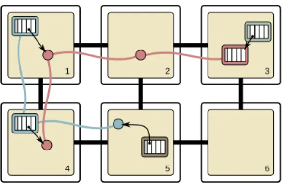
3.4 A simple data structure distributed over six Chunk Peers. . . 52

3.5 Reference Tree for Figure 3.4. . . 54

3.6 Reference Tree configuration needed to grant a Modify privilege. . . 55

3.7 A race between two Modify privilege requests. . . 57

3.8 An example of Reference Tree expansion. . . 58

3.9 Garbage collection example. . . 61

4.1 Distributed Reference Tree state. . . 65

4.2 Chunk State as a copy moves to another node. . . 71

4.3 The components of the Chunk Exchange layer. . . 74

4.4 Chunk and Channel States during Reference Tree expansion. . . 80

(12)

4.6 Chunk and Channel States for the process of granting a Modify request. . . 83

4.7 The T bit protects against premature collection of sub-graphs of chunks. . . 87

4.8 Garbage collection example for a node with no chunk copy. . . 88

4.9 Garbage collection example for a node with a chunk copy. . . 89

4.10 A cycle spanning multiple nodes. . . 91

5.1 The SCVM ecosystem. . . 94

5.2 SCVM bytecode forfactorial(n). . . 96

5.3 Screen shot of the Quickr photo organization tool. . . 99

5.4 Screen shot of the PhotoChop photo editing tool. . . 99

5.5 Tasklet Trading Service . . . 103

5.6 FrameContext chunks. . . 105

6.1 Clients using server-side path de-referencing. . . 108

6.2 Data transferred streaming a video. . . 109

6.3 Radius Pre-fetching Performance. . . 110

6.4 Shape Pre-fetching Performance. . . 112

(13)

List of Listings

2.1 Client-side playback algorithm for ChunkStream. . . 38

4.1 (J?)Channel Proxy bootstrap procedures. . . 70

4.2 B?Channel Proxy bootstrap procedures. . . 70

A.1 The FC Transition. . . 130

A.2 The FE Transition. . . 130

A.3 The RQC Transition. . . 130

A.4 The RQE Transition. . . 130

A.5 The RSC Transition. . . 130

A.6 The RSE Transition. . . 131

A.7 The FRSE Transition . . . 131

A.8 The GRR Transition. . . 131

A.9 The GRM Transition. . . 132

A.10 The GCLT Transition. . . 132

A.11 The GCD Transition. . . 132

A.12 The GCRG Transition. . . 132

(14)

(15)

List of Tables

3.1 Chunk API exposed by the Chunk Runtime. . . 49

4.1 Chunk Exchange Protocol Request messages. . . 67

4.2 Chunk Exchange Protocol status messages. . . 68

4.3 The Channel States of the Chunk Exchange Protocol. . . 69

4.4 Transition table of the Channel Proxy FSM. . . 72

4.5 The six types of requests. . . 74

4.6 Major Chunk State bits . . . 75

4.7 Privilege bits . . . 75

4.8 The Reactor reaction table. . . 78

4.9 Reactor function descriptions. . . 79

4.10 Reactor Error Types . . . 80

6.1 Table of raw Radius Pre-fetch performance values. . . 111

6.2 Shape Table for Elephants Dream. . . 111

(16)

(17)

Chapter 1

Introduction

In the past few years, the computer industry has seen the growth of three new computing substrates: elastic cloud computing, massively multi-core computing, and general-purpose GPU computing. At a high-level, these three substrates are wildly different. Elastic cloud computing systems like Amazon’s EC2 [8] and Microsoft’s Azure [70] provide dynamically expandable clusters of hosts, each connected over a virtualized network. Massively multi-core processors like the Tilera TILE [91] series of processors provide a plethora of processor cores connected by on-chip buses and local caches. General-purpose GPUs like NVIDIA’s Tesla [64] provide an abundance of ALUs connected by a hierarchy of memories.

While the granularity and specifics of these new substrates differ, what is common to all of them is (1) an abundance of processing elements and (2) programmer-visible communi-cation and storage hierarchies whose proper utilization determines both correctness and performance of applications. For example, in the cloud, intra-core operations are faster than intra-host operations, which are faster than inter-host operations. Likewise, in the GPU, communication and data sharing within a single processing element is fast compared to communication and sharing processing between elements, which itself is fast compared to CPU to GPU communication.

In contrast to “normal” CPU-based platforms that automatically manage the memory and communication hierarchy for correctness and high performance, programmers must carefully manage the communications and storage hierarchies of the new computing sub-strates so that processing elements are continually fed with instructions and data. Typically this is done by manually managing communication and data placement with

(18)

substrate-specific frameworks to ensure that related computations are on processing elements close to each other in the computing substrate and that computations “fit” into the variously sized storage buckets that each level of the substrate provides. The substrate-specific frameworks force programmers to use special programming paradigms that chain their programs to particular configurations of specific machines. This is unfortunate because it takes flexibility away from programmers by restricting how they may solve their problems.

1.1 Program Structure versus Platform Structure

To better understand the predicament of modern computing substrates, it is instructive to review how software and hardware are structured and how they work together. At the programming-language layer, programmers use structuring mechanisms provided by their favorite language to construct models of the real-world problems they need to solve. For example, all programming languages provide functions to organize algorithms and control execution of code as well as record types to organize related data. Functions can be further decomposed into basic blocks connected by explicit flow control primitives. Object-oriented languages extend the model by providing objects that tie code and related methods together. At this top-layer, programming language structuring mechanisms allow programmers to optimize for maintainability and readability of code by keeping related concepts near each other in source code—leading to locality of concepts in the program source—as well as build layers of abstraction that hide unnecessary details that would otherwise hinder understanding of the program.

Explicit structure is also rich at the hardware layer. At this level, structure reflects finite physical resources with different performance characteristics, sizes, and availability. For example, memory is organized into a hierarchy of fast and small caches spilling over into multi-channel DRAM main-memories, all backed by slow, but potentially enormous, disks and network file systems. Data that are in the same cache will be equally fast to access, while those that are in different levels of the hierarchy will have slower access times. A program whose working set can fit within a high-speed cache will be orders of magnitude faster than a program that must go out to main memory, or worse yet, swap. Similarly, computation power is organized into threads that execute on particular cores embedded within a heterogeneous communication topology. Two threads assigned to the

(19)

same processor or chip package will be able to more easily communicate and synchronize than two threads in cores in different places on the network. Similarly, threads on the same network will be able to more easily communicate and synchronize compared to threads that must communicate over the wide-area Internet. In general, the closer two related items are to each other in the memory or processor network, the faster the application will be able to combine and use the items. However, cost and power concerns constrain the fast components to be small relative to the rest of the system, forcing the application and operating system to continually copy data into and out of the fast components in order to maintain high performance. Ergo, the hardware has a natural, if non-linear, “distance” metric between components.

In contrast, the middle of the computing stack—the machine abstraction consisting of machine code instructions operating on a flat address space of memory—is largely devoid of explicit structure. Programs are compiled into strings of instructions that operate in a flat virtual memory address space on flattened data structures. The flat address space obscures the relationship between parts of a program to the operating system: because there is no requirement to keep related code and data close to each other, they are often scattered throughout the address space. Even if related code and data were in similar locations, the lack of explicit typing of data in memory makes it difficult to divine exact relationships since the processor cannot distinguish pointers from integers until it uses them [26]. The

Machine Interface Programming Language Operating System Hardware class Person { ... }

int decode(FILE *stream) { ...

}

struct Node { struct Node *next; struct Node *prev; } VM Procs Caches DRAM Disks Cores Functional Units Tracks Sectors

(20)

flat address space also obscures from the program the costs of different data structures and code organizations since the machine model offers no portable way of exposing the sizes, and consequently, the predicted placement or fragmentation of objects within the hardware components in the system. As Figure 1.1 illustrates, the machine abstraction forms the structural bottleneck between the highly structured ends of hardware and software.

1.2 Mapping Structure

Since compute resources are of finite size and there is a cost associated with moving data between different components of the machine, a key problem in maintaining high performance in a computer system is ensuring that related parts of a program are located “close” to each other. When resource characteristics and limits are known, e.g., exactly how big a component can get before it overflows a level in the storage hierarchy or exactly how close two related threads of computation need to be to maintain high performance, programmers can build systems that exploit resources efficiently. For example, once a spinning hard disk has positioned its disk read head over a track, it can read or write the entire track at very high speed, but will not be able to perform any reads or writes while moving (seeking) the head to another track. As such, file systems have evolved to collect many small reads and writes and coalesce them into a single large read or write to avoid costly head seeks.

1.2.1 Optimization within the Flat Middle

Given that both programs and computers are highly structured, we would like to cast the locality problem to one of mapping program structure onto machine structure, ideally in a machine-portable way. Unfortunately, the unstructured machine abstraction makes the mapping harder since program structure is obscured by the implicit structure of machine code and the machine’s structure is obscured by the flat memory address space. Indeed, it is because of how the traditional machine abstraction obscures structure that modern computing substrates each come with their own frameworks and structuring abstractions. The design choice to connect two highly structured layers with an unstructured inter-mediary layer made sense at one time because the two layers have orthogonal structure and could be engineered independently. Indeed, for the past several decades, computer

(21)

scientists and engineers have been able to build elegant optimizations at each end of our hourglass that provided acceptable performance despite the thin middle. At the hardware-level, caches trace program execution and place commonly used code and data in fast memory banks close to the processor, essentially dynamically extracting “close” code and data from patterns in the memory access stream. At the software layer, optimizing compil-ers remove unnecessary structure from applications by putting related code in the same basic blocks. The flattened code essentially groups related functions into sequential streams of instructions, better matching the cache-enhanced flat execution environment by enabling address-based caches to pre-fetch more related data.

1.2.2 Breaking the Abstraction

These optimizations, however, can only extract so much structure from the executing program. As computers evolved, simple caches and hardware-agnostic optimizations were no longer good enough to fully utilize new hardware and the industry resorted to breaking through the clean machine code abstraction.

For example, in the early 1990’s compilers were tuned for the pipelines, delay slots, and cache configuration for specific processors [22, 93], leaking specific hardware details through the machine language abstraction up to the program and, consequently, pairing binaries to specific implementation details of particular machines. Recent work on cache-oblivious algorithms and data structures [37] has reduced the need to worry about the specifics of any cache—though cache-oblivious algorithms do assume that there is some hierarchy in the memory system. Demaine [30] surveys early work in the area and shows that for many problems, cache-oblivious algorithms can meet the theoretical running times of cache-aware algorithms. Unfortunately, cache-oblivious algorithms require program code to be structured in a particular way that limits how programmers may implement their algorithms.

Similarly, very long instruction word (VLIW) processors [35] expose all of the functional units in the processor directly to the user program and require the user program (or compiler) to schedule everything. VLIW failed in the marketplace for two reasons. First, each VLIW processor had a different number of functional units, and as such required different binaries for each generation of the same processor family, reducing portability.

(22)

Second, compilers could not statically fill functional units any better than normal super-scalar processors.

1.2.3 Dissolving the Machine Abstraction

The systems of the previous section all break the machine abstraction by exposing low-level information to the highest low-levels of the computation stack, where it was believed that a compiler could make the most use of the extra information. However, these fix-ups are unsuccessful because there is only so much optimization that can be applied to the instruction stream of a single program. As the computing environment continues to evolve, we may be faced with problems that may not be solvable by simply considering a single stream of instructions, but rather may require a more holistic approach to how applications are structured and how they may interact with increasingly complex machines. For example:

• Users increasingly interact with video and other streaming media that passes through the processor once, suffering high memory latencies to bring data into the processor as well as polluting the cache with now-stale data. The program may work more efficiently if the processor pre-fetches data into a reserved subset of cache lines while leaving other lines alone. In order to do so, we need a way to analyze the structure of the streaming media application and have a run-time system schedule memory reads ahead of the application.

• As processor frequency scaling has hit a power-induced limit, we have seen a resur-gence in distributed and parallel computing. In the flat model, the program must manage its own execution and manage the lifetime of threads. Programmers would be far more efficient if the system could identify program areas that may potentially run in parallel and use that information to automatically manage thread pools for the application.

• Many modern applications also make use of computing clusters that scatter parts of the application across many machines. Is there a way to allow a run-time system to optimize placement of components based on the dynamic needs of applications?

(23)

In all of these cases, the application may be able to run more efficiently if the operating system can more easily analyze the structure of the application and use this information to schedule resources proactively. Rather than add more features to our existing machine abstraction, it might make sense to have a new abstraction that takes into account the need for run-time optimization by the operating system.

1.3 Thesis: A Structured Computing Model

This thesis explores the hypothesis that preserving and exposing structural information about both software and hardware across the machine abstraction will make it easier to build and maintain broad classes of applications running on modern computing substrates. Rather than design ad-hoc APIs that cater to specific problem domains and application designs, we would like a new abstraction that exposes relevant structure in a way that run-time support software can leverage to manage and optimize applications, yet itself is application-generic and machine-generic. In other words, we explore whether expanding the thin middle in the structural hourglass of Figure 1.1 makes it easier to build application-generic supporting layers for the variety of modern computing substrates.

1.3.1 Principles

The design of the abstractions and mechanisms detailed in this thesis are guided by two core principles influenced by the observations of the previous few sections:

Structural Transparency Our primary hypothesis is that an abstract notion of structure will enable run-time systems to automatically and efficiently map program structure onto the machine structure of modern computing substrates. When structure is transparent to the runtime, it provides a foundation on which to exploit structure for efficiency and optimization. As such, our abstractions and mechanisms should be designed to make structure explicit.

Structural Navigability The exposed structure encouraged by the Structural Transparency principle is only useful if the structures are logically laid out. A data structure whose interior details seem randomly designed will be harder to exploit than one where related information is localized within containers, where paths to required data are

(24)

clear-cut, and where there are obvious contours for sub-setting the data structure to make its run-time footprint smaller.

Structural Navigability is the principle that computation should be able to efficiently navigate through a data structure to access and manipulate only the parts relevant to the computation at hand, while ignoring those parts that are irrelevant. The abstractions and mechanisms we provide must encourage developers to employ those abstractions to express relations and locality that may otherwise be lost in translation between the program layer and the machine layer.

The Structural Navigability and Structural Transparency principles build upon each other, as optimizations that exploit Structural Navigability depend on Structural Transparency as a foundation. At the same time, those optimizations may remove negative performance impacts of Structural Transparency, thus encouraging developers to refactor existing data structures into more finely-grained data structures and potentially enabling another round of Structural Navigability-based optimization.

1.3.2 Contributions

This thesis makes two major technical contributions: the Chunk Model, an application-generic, platform-application-generic, structure-preserving memory model, and the Chunk Platform, a prototype implementation of the Chunk Model.

The Chunk Model

This thesis explores our hypothesis through the Chunk Model, a structure-preserving memory model. In the Chunk Model, memory comprises a universe of individually-identified, fixed-sized chunks. The Chunk Model does not have an address space: instead chunks reference other chunks with explicitly-marked links containing the identifiers of other chunks. Applications express their multidimensional data structures as graphs of explicitly linked chunks rather than flattened data structure connected by implicit address pointers.

We chose the Chunk Model to explore application- and platform-generic structuring mechanisms for three reasons. First, graphs of chunks are generic enough to build any pointer-based data structure. Applications using the Chunk Model only need to translate

(25)

Figure 1.2: A universe of chunks divided into finite subsets. Each subset may be hosted by independent machines. Note that some links extend beyond the borders of the figure.

their internal structures to chunk-based ones, rather than use platform-specific structuring primitives. Second, the Chunk Model forces objects larger than one chunk to be expressed as graphs of chunks. In doing so, the application explicitly exposes its structures to run-time layers, enabling those run-time layers to optimize execution of the chunk-based applications using information in the chunk graph. Third, the use of identities rather than addresses insulates the Chunk Model from the constraints of any platform-specific addressing scheme. As shown in Figure 1.2, it is possible to divide the universe into bounded, potentially shared, subsets of chunks distributed among independent hardware nodes. While a particular piece of hardware may only be able to access its finite subset of the universe of chunks at any given time, clever management and translation of “universal identities” to local identifiers ensure that nodes using the Chunk Model may migrate chunks between themselves, enabling each node to have a finite window on the infinite universe of chunks.

The Chunk Platform

The Chunk Platform implements the Chunk Model while embracing the distributed and network-oriented nature of modern computing substrates. Each node in the Chunk Platform runs a node-local Chunk Runtime that manages the chunk-based applications on the node and provides those applications with a Chunk API that give them a window into the universe of shared chunks.

(26)

The Chunk Runtime on each node can only hold a subset of the shared universe of chunks. To give applications access to the whole universe of chunks, the Chunk Runtime on each node uses a low-level networking protocol called the Chunk Exchange Protocol to manage the distribution of chunks. The Chunk Exchange Protocol enables nodes to divvy up the universe of chunks among Chunk Runtimes, as illustrated by Figure 1.2. The Chunk Runtime uses the Chunk Exchange Protocol to take care of coherent caching of chunks, consistent updates to chunk copies, and reclamation of chunks as computations no longer need them. The Chunk Exchange Protocol uses Reference Trees, an abstraction introduced by Halstead [47], to manage chunks distributed across multiple Chunk Runtimes. Reference Trees abstract and summarize the configuration of the distributed chunk universe in a way that reduces the amount of local state each Chunk Runtime must maintain. Reference Trees also provide convenient mechanisms for maintaining consistency of chunk updates as well as for garbage collection of chunk resources.

The Chunk Platform serves as a prototyping platform to evaluate and validate the Chunk Model. As such, the Chunk Platform supports a variety of applications ranging from those that use chunks only as a distributed data store to SCVM, a virtual machine architecture that uses the Chunk Model for computation.

Other Contributions

While we primarily use the Chunk Platform to evaluate the Chunk Model, our implementa-tion of the Chunk Platform provides several other contribuimplementa-tions:

• a wire format for sharing graphs of chunks,

• a distributed protocol implementing a sequentially consistent memory model for shared graphs of chunks,

• a distributed garbage collection algorithm of chunk graphs that can collect cycles distributed across many nodes,

• a reference compiler that targets chunks while hiding the chunk model from the programmer, and

(27)

In most cases, while these contributions make use of our particular chunk abstraction, they can be adapted to traditional reference-based object systems and thus are useful independent of the Chunk Platform.

1.3.3 Thesis Outline

The next chapter details the Chunk Model. Chapter 3 outlines the Chunk Platform at a high level. A lower-level description of the Chunk Platform, including details of its application-generic run-time services, consistency model, and garbage collection algorithm, follows in Chapter 4. Chapters 5 and 6 evaluate the Chunk Platform through building chunk-based applications and evaluating chunk-chunk-based optimization techniques, respectively. After evaluation, the thesis continues with a review of related work in Chapter 7 and concludes with future work in Chapter 8.

(28)

(29)

Chapter 2

The Chunk Model

This thesis explores the Chunk Model as a more structured replacement for the unstructured memory abstraction of current computing models. The Chunk Model extends the standard von Neumann approach to computing with a structured memory rather than a flat memory. In doing so, the Chunk Model enables a structured way of storing everything, from data to computer programs to the run-time state of those programs.

The Chunk Model differs from the current flat memory abstraction in three ways. First, the Chunk Model replaces memory as a flat array of bytes with an unbounded universe of chunks. Chunks are fixed-size, so large data structures must be represented as graphs of many inter-referencing chunks. These graphs embody the Structural Transparency Principle and enable the Chunk Model to capture application-specific structure in a generic way.

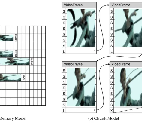
Second, the Chunk Model replaces pointer arithmetic as a way of navigating memory with de-referencing explicitly-typed links between chunks. Chunks in the Chunk Model have identities, not addresses; the only notion of distance between chunks stems from the links between them rather than the nearness of addresses. Explicit links serve our transparency goal, since it allows run-time services to read graphs of chunks without complex analysis to disambiguate integers from pointers, while requiring chunk identities force the use of links to identify chunks, since there is no way to obtain a chunk except by de-referencing a chunk identifier. As Figure 2.1 illustrates with the last four frames of a video, rather than placing arbitrary data as a monolithic binary in the flat memory address space, the Chunk Model compels applications to place their data in a graph of chunks. At

(30)

• • • 0x200 0x300 0x400 0x500 0x600 0x700 0x800 0x900 • • • 0 x4 0 0 0 x5 0 4 0 x7 0 2 0 x0

(a) Flat Memory Model

S S S S S S S L VideoFrame S S S S S S S L VideoFrame S S S S S S S L VideoFrame S S S S S S S X VideoFrame (b) Chunk Model

Figure 2.1: A comparison of traditional flat-memory model and the Chunk Model using a video stream as an example. In the flat model, video frames are copied into the flat memory and connected by addresses at the end of frames. In the Chunk Model, individual frames are placed in chunks that are connected by explicit links.

run-time, rather than following pointers to specific addresses or computing addresses using pointer arithmetic, applications follow links inside chunks to other chunks. For example, in the figure, while an application in the flat model uses the integer addresses at the end of each frame to find the next frame, an application in the Chunk Model follows explicitly marked links.

Third, the Chunk Model replaces on-demand paging of memory with explicit placement of chunks in the memory hierarchy of a computing substrate. Just as current computers can address much more memory than they may physically possess, any given chunk-based com-puter is only able to reference a finite subset of the universe of chunks. Explicit placement of chunks enables substrate-specific run-time systems to customize chunk placement to best fit hardware-imposed constraints. In the example of Figure 2.1, the machine would load chunks into memory as the application walks down the linked list of frames. Compared to a virtual address system where pages are loaded when accessed, a chunk-based machine may anticipate paths taken in the chunk graph as hints to load chunks before they are needed.

(31)

Grand Teton Nat ional Park is l ocated in north western Wyoming , south of Yell owstone Nationa l Park. The pa S S S S S S S L TextChunk S S S S S S S S ImageChunk #73 #163 #73

Figure 2.2: Two chunks with a link between them. The gray bar indicates the start of the chunk and contains the type hint. Each slot is typed with a type field (Sfor scalar andLfor links).

2.1 Chunks

At the core of the Chunk Model is the chunk data type. A chunk is an ordered, fixed-sized array of fixed-sized slots. The number of slots in a chunk and the width of each slot is “universal” and shared by all nodes in the system.

Each slot consists of a type tag and a fixed-width data field. The type indicates how the data field should be interpreted: as an empty slot (X), as scalar binary data (S) or as a reference (“link”, L) to another chunk. Scalar values are uninterpreted byte arrays; applications may store any scalar value they wish in a slot as long as that scalar value fits in the size limits of the slot. Chunk links are used to create large data structures out of graphs of chunks. Explicit typing of slots helps chunks achieve our goal of transparency since run-time analysis of the chunk graph need only look at the slot types to determine what are links and what are scalars. Chunk links are simply slots explicitly typed as references and filled with the identifier (chunk ID) of the referent chunk. Chunk IDs are opaque, network-neutral reference to chunks that are mapped to hardware locations at run time. Maintaining a level of indirection between chunk references and hardware enables platform-generic placement and migration of chunks.

Each chunk is annotated with a chunk type. The chunk type is a slot that serves as a specification of the semantics of the slots of the chunk. Applications and libraries use the chunk type as a hint on how to interpret the chunk’s slots or for run-time data type checks.

Figure 2.2 illustrates two chunks with N = 8 slots. The chunk on the left is a TextChunk, which has the specification that the first N − 1 slots are scalar UTF-8 encoded text and that

(32)

S S S S S S S L ImageChunk S S S S S S S L ImageChunk S S S S S S S L ImageChunk S S S S S S S X ImageChunk

Figure 2.3: A large image spills over into multiple chunks.

the last slot is a link to a related chunk. The TextChunk links to an ImageChunk, whose specification states that the first N − 1 slots are packed binary data of a photograph, and that the last slot is either scalar data or a link to another ImageChunk if the encoding of the photograph does not fit in a single chunk.

Chunks may also be used as unstructured byte arrays by simply filling slots with uninterpreted binary data. For example, as shown in Figure 2.3, a larger version of the photograph in Figure 2.2 may be split across a linked list of four ImageChunk chunks.

2.2 Why Chunks?

This thesis uses chunks as its foundation data type for three reasons—generic structuring primitives, opaque identities, and fixed-sizes—each detailed in the subsequent paragraphs.

2.2.1 Transparent and Generic Structure

The first reason why we use chunks is that chunks embody a flexible, reference-based interface that can be used to build, link together, and optimize larger data structures one block at a time. Chunks can be used to implement any pointer-based data structure, subject

(33)

to the constraint that the largest single element fits in a single chunk. Small chunks force the use of fine-grained data structures, creating many more decision, and optimization, points over whether or not to fetch a particular portion of a data structure.

Since the chunk interface is fixed and chunk links are network-neutral references, chunk-based data structures can be shared between any two nodes that use chunks without worrying about format mismatches. The chunk abstraction and the chunk interface is the embodiment of the Structural Transparency Principle of this thesis because chunks expose structure through the graph induced by the explicitly marked links. System-level code—like that handling coherence, caching, and optimization—can operate at and optimize the layers underneath the application using only the structure exposed by chunks without needing to worry about the exact semantics of each slot’s value.

2.2.2 Identities Instead of Addresses

The second reason for using chunks is that chunk IDs are opaque references and not addresses. Opaque chunk IDs serve to break the abstraction of the flat virtual memory address space as well as provide a level of indirection between chunks and the locations where they are stored. The former is important because it removes the assumption that virtual addresses near each other have anything to do with each other, a fallacy because the contents of one virtual address may be in a L1 cache and available in a cycle while the next word in the virtual memory may be on disk and take millions of cycles to fetch. Breaking up a data structure into chunks makes it explicit that crossing a chunk boundary may impose a performance hit. Moreover, address arithmetic no longer works, meaning that data structures can only be accessed via paths in the chunk graph, rather than randomly. Doing so exposes the true cost of data structures, since (1) it is necessary to build helper chunks to access large data structures and (2) those data structures reflect, in chunk loads, the costs of accessing random items in memory normally obscured by the virtual memory subsystem.

The indirection property of opaque chunk IDs is important for two architectural reasons. First, it enables chunks to be moved around not only between processes, but also between nodes in the same network, giving a chunk-based run-time system the flexibility to not only place chunks within the memory hierarchy of one node, but also to place chunks on other nodes in the computation substrate. Second, using opaque chunk IDs frees the Chunk

(34)

Model from the inherent finiteness of an address-based namespace. While an individual node may be limited in the number of chunks it may hold due to the size of its own memory, there is no inherent limit on the number of chunks in the Chunk Model’s universe of chunks: clever management and reuse of local chunk IDs by an implementation of the Chunk Model can provide an finite sliding window on the infinite universe of chunks.

2.2.3 Fixed Sizes

The third reason for using chunks is that since chunks comprise of a fixed number of fixed-sized slots, there is a limit to the total amount of information that a single chunk can hold as well as a limit to the number of chunks to which a single chunk can directly link. While fixed sizes may be seen as a limitation, size limits do have certain benefits. In particular, fixed-sized chunks, when combined with the reference properties of chunks, give rise to three useful geometric notions that aid run-time understanding of chunk data structures.

First, since building large data structures requires building graphs of chunks, the Chunk Model has an inherent notion of size. At the software level, size measures the number of chunks that comprise the entire data structure. At the hardware level, size measures the number of chunks that fit within a particular hardware unit. Knowing the relative sizes of data structures and hardware provides chunk-based systems with information to inform chunk placement algorithms. Small data structures are those that fit within the constraints of a hardware unit; large data structures are those that overflow a particular hardware unit and whose placement must be actively managed.

Second, chunks give rise to dual concepts of distance. At the data structure level, distance is the number of links between any two chunks in a data structure. At the run-time level, distance is the number of links followed during a particular computation. In an efficient data structure, related data are on chunks a small distance away from each other. Distance, in other words, leads to the notion of a local neighborhood of related chunks, both for passive data structures as well as for chunks needed for a given computation. Chunk-based systems may use distance information to infer which chunks should be placed together.

Lastly, chunks embody structure as a way of constraining the relationship between size and distance. Particular design choices may lead to differently-shaped data structures. Each of the different shapes may be useful for different problem domains. For example, the large

(35)

(a) 2-D Array (b) Progressive

Figure 2.4: Alternative chunk structures for storing image data.

image in Figure 2.3 is represented as a linked list of chunks, a long data structure that is appropriate if the image data can only be accessed as a single unit. If the image codec has internal structure, other choices may be better. For example, if the image is constructed as a two-dimensional array of image blocks, a 2-D array of chunks may be appropriate. If the image is encoded using a progressive codec where the more data that one reads the sharper the image gets, then a more appropriate chunk structure may be one that exposes more chunks as an application digs deeper into the data structure. As shown in Figure 2.4, the particular choices each beget a different shape, which may be used to more efficiently discover how the chunks will be used and inform how those chunks should be placed within the computing hardware.

2.2.4 Chunk Parameters

While the chunk abstraction requires the number of slots and the length of each slot to be fixed, this thesis does not advocate any particular binding of those parameters. Each computing substrate may require its own particular set of ideal chunk sizes:

• when running on top of a typical computer, chunks that fit within 4KB pages may be ideal;

• a computation distributed across a network may require chunks fit within 1,500 byte or 9,000 byte Ethernet frames in order to avoid packet fragmentation; while

(36)

• a massively multi-core machine may work best when a chunk fits in a small number of chip-network flits.

All that matters for the abstraction to work is that a particular choice is made, that the choice enable each chunk to have at least a small number of slots1_{and that the same choice}

is used throughout the computing substrate.

2.3 Example Chunk Structures

The Chunk Model enables the construction of application-specific data structures using a generic foundation; the only problem is figuring out how to represent application-specific data in chunks in a way that adheres to the Structural Navigability Principle. To help ground how chunks may be used consider two disparate problems: video streaming and general computing.

2.3.1 ChunkStream: Chunks for Video

Video is an ideal candidate for structured computing systems since video data is inherently structured, yet must be flattened into byte-oriented container formats for storage and transfer in traditional computing systems. Video container formats serve as application-specific structuring mechanisms in that they enable a video player to search within the byte-oriented video file or stream and pick out the underlying video codec data that the player needs to decode and display the video. Each container format is optimized for a particular use case and, as such, may offer only certain features. Some, like MPEG-TS [1], only allow forward playback, while others like MPEG-PS [1], AVI [69], and MKV [67] also allow video players to seek to particular locations, while others, like the professional-level MXF container format [3] are optimized for frame-accurate video editing.

ChunkStream’s video representation is guided by the observation that video playback consists of finding frame data in the order it needs to be decoded and displayed. If the representation of each video stream were a linked list of still frames, playback would be the act of running down the linked list.

1_{The lower bound of the number of chunks per slot is two, making chunks akin to LISP}_cons_{cells, but we}

find that a lower bound closer to 8 is much more useful since it gives applications more room to distinguish between slots for their own purposes.

(37)

Index Tree Backbone Lane Markers Frame Data Lane #0 (HD) Lane #1 (low-bandwidth)

Frame #1 Frame #2 Frame #3 Frame #4

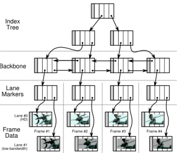
Figure 2.5: Chunk-based video stream representation used by ChunkStream. LaneMarker chunks represent logical frames and point to “lanes” composed of FrameData chunks. Each lane represents the frame in different formats, e.g. using HD or low-bandwidth encodings. Links to StreamDescription chunks and unused slots at the end of chunks are not shown.

With those observations in mind, ChunkStream represents video streams with four types of chunks, as illustrated in Figure 2.5. The underlying stream is represented as a doubly-linked list of “backbone” chunks that connect representations of individual frames. The backbone is doubly-linked to allow forwards and backwards movement within the stream. For each frame in the video clip, the backbone links to a “LaneMarker” chunk that represents the frame.

The LaneMarker chunk serves two purposes. First, it links to metadata about its frame, such as frame number or video time code. Second, the LaneMarker links to “lanes” of video. A lane is a video sub-stream of a certain bandwidth and quality, similar to segment variants in HTTP Live Streaming [81]. A typical LaneMarker might have three lanes: one high-quality high-definition (HD) lane for powerful devices, a low-quality lane suitable for playback over low-bandwidth connections on small devices, and a thumbnail lane that acts as a stand-in for frames in static situations, like a timeline. ChunkStream requires that each lane be semantically equivalent (even if the decoded pictures are different) so that the client may choose the lane it deems appropriate based on its resources.

Each lane takes up two slots in the LaneMarker chunk. One of these lane slots contains a link to a StreamDescription chunk. The StreamDescription chunk contains a description

(38)

1 defplay(tree_root , frame_num): 2

3 # Search through the IndexTree:

4 backbone = indextree_find_frame(tree_root, frame_num) 5

6 whileplaying:

7 # Dereference links from the backbone down to frame data:

8 lm_chunk = get_lane_marker(backbone, frame_num)

9 lane_num = choose_lane(lm_chunk)

10 frame_data = read_lane(lm_chunk, lane_num) 11 # Decode the data we have

12 deocde_frame(frame_data)

13

14 # Advance to next frame in backbone:

15 (backbone, frame_num) = get_next(backbone, frame_num)

Listing 2.1: Client-side playback algorithm for ChunkStream.

of the lane, including the codec, stream profile information, picture size parameters, stream bit rate, and any additional flags that are needed to decode the lane. Lanes are not explic-itly marked with identifiers like “HD” or “low-bandwidth”. Instead, clients derive this information from the parameters of the stream: a resource-constrained device may bypass a 1920x1080 “High Profile” stream in favor of a 480x270 “Baseline” profile stream while a well-connected desktop computer may make the opposite choice. As an optimization, ChunkStream makes use of the fact that in most video clips, the parameters of stream do not change over the life of the stream, allowing ChunkStream to use a single StreamDescription chunk for each lane and point to that single chunk from each LaneMarker.

The other slot of the lane points to a FrameData chunk that contains the underlying encoded video data densely packed into slots. If the frame data does not fit within a single chunk, the FrameData chunk may link to other FrameData chunks.

Finally, in order to enable efficient, O(log n) random frame seeking (where n is the total number of frames), the top of the ChunkStream data structure contains a search tree, consisting of IndexTree chunks, that maps playback frame numbers to backbone chunks.

Video Playback

Listing 2.1 shows the algorithm clients use to play a video clip in ChunkStream. A client first searches through the IndexTree for the backbone chunk containing the first frame to play. From the backbone chunk, the client follows a link to the LaneMarker for the first frame, downloads any necessary StreamDescription chunks, and examines their contents to determine which lane to play. Finally, the client de-references the link for its chosen lane to

(39)

fetch the actual frame data and decodes the frame. To play the next frame, the client steps to the next element in the backbone and repeats the process of finding frame data from the backbone chunk.

Advantages of the Chunk Model

An advantage of exposing chunks directly to the client is that new behaviors can be im-plemented without changing the chunk format or the protocols for transferring chunks between the video player and the video server. For example, the basic playback algorithm of Listing 2.1 can be extended with additional features by simply altering the order and number of frames read from the backbone. In particular, a client can support reverse play-back by stepping play-backwards through the play-backbone instead of forwards. Other operations, like high-speed playback in either direction may be implemented by skipping over frames in the backbone based on how fast playback should proceed.

It is also possible to implement new server-side behaviors, such as live streaming of real-time video. Doing so simply requires dynamically adding new frames to the backbone and lazily updating the IndexTree so that new clients can quickly seek to the end of the stream.

2.3.2 CVM: Computing with Chunks

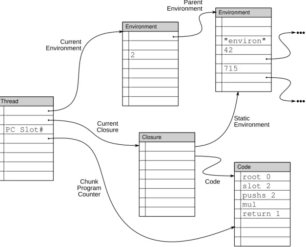
While ChunkStream is an example of using chunks for data structures, chunks are also a useful foundation for computation. One way to use chunks for computation is to make use of the standard “stored program” computer trick and use chunks as the backing store for all state—including executable code, program data, and machine state. Figure 2.6 shows an example computation expressed in chunks for a computing system based on closures and environments2. We call this the CVM data structure, since it represents a chunk-based virtual machine.

At the root of the data structure is a Thread chunk. The Thread chunk contains all of the run-time information that the computation needs: a link to the current environment (stored in Environment chunks), a link to the currently running code (enclosed in a Closure chunk), a “program counter” indicating where the next instruction can be found (pointing to Code chunks), a link to the previous invocation frame (e.g., the previous function on

(40)

Code pushs 2 root 0 slot 2 mul return 1 Environment 2 Environment "environ" 42 715 Thread PC Slot# Current Environment Chunk Program Counter Parent Environment Static Environment Code Current Closure ••• ••• Closure

(41)

the stack), as well as slots for temporary storage (e.g., machine registers or machine stack). Each Environment chunk represents a scoped environment for computations; each slot in the Environment chunks represents a program variable. The Closure chunk points to both the closure’s static environment as well as its code.

A machine using the CVM data structure starts a cycle of computation by de-referencing program counter chunk and then reading the instruction at the program counter slot. The instruction may read or write temporary values in the Thread chunk or modify chunks linked to by the Thread chunk. After the instruction executes, the program counter is updated to point the next instruction, which may be in another chunk as in the case of branches or jumps.

Migration with CVM

A consequence of the Chunk Model only allowing chunks to reference other chunks through links is that CVM computations can only access chunks transitively linked from the root Thread chunk. This constraint forces the CVM data structures to be self-contained: each Thread chunk necessarily points to all of the code and data that the computation uses. A consequence of this property is that it is easy to move threads of computations between nodes running a CVM computation.

To migrate computation between CVM instances, the source VM need only send the root Thread chunk to the destination VM. As the destination VM reads links from the chunk, it will request more chunks from the source VM until it has copied enough chunks to make progress on the computation.

In many ways, the CVM migration strategy is similar to standard on-demand paging schemes. However, it is possible to exploit two properties of the CVM chunk representation to speed up migration. First, the fine-grained nature of the CVM data structure allows the migration of only small portions of running programs, such as an individual function, individual data objects, or even just the code and objects from a particular execution path, rather than an entire binary and its resident memory. Second, it is possible to exploit locality exposed by explicit links during the migration process and send all chunks within some link radius of the Thread chunk all at once, under the assumption that chunks close to a computation’s Thread chunk are likely to be used by that computation. For example, in

(42)

Thread T1 Thread T2 Thread T3

Figure 2.7: Three threads operating in a chunk space with their volumes of influence for Di= 1highlighted. Threads t1and t2are close to each other and must to be synchronized,

while thread t3may run in parallel with the other threads.

Figure 2.6, the source might send the Thread chunk and the three chunks to which it links to the destination.

Volume of Influence

If one makes a few assumptions on the nature of CVM code, the fixed-size nature of chunks leads to interesting bounds on the mutations that a CVM computation can make. Suppose that CVM code consists of a sequence of instructions packed into Code chunks and each instruction can only access chunks some bounded distance Di from the computation’s

Thread chunk. Each instruction may only bring a distant chunk closer by at most Di

links, i.e., by copying a chunk reference from a chunk a distance Di away and placing it

temporarily in the root Thread chunk. Since Code chunks, like all chunks, have a fixed size, there is a limit to number of instructions in each Code chunk and, correspondingly, a limit to how many chunks the instructions in the Code chunk can access before the computation must move on to another Code chunk. We call the limited set of chunks that the thread can access the volume of influence of the Thread. Suppose are N instructions in each chunk. If Thread chunks of two threads have roots that are 2N Diapart from each other in the chunk

graph, then they cannot influence each other during the execution of their current Code chunks. If two threads are closer than 2N Di, their volumes of influence may overlap and

(43)

may need to be considered together by the hardware management and chunk placement layer.

For example, consider Figure 2.7, in which three threads execute in a chunk space. Threads t1 and t3 are far away from each other in the space and may be able to run

concurrently without competing for resources like memory bandwidth. In contrast, threads t1and t2have overlapping volumes of influence and must time-share memory bandwidth

and synchronize access to their shared chunks. The substrate’s run-time system may be able to use this information to, e.g., place t1and t2on the same processor core so they can

share chunks using higher-performance local communication primitives, while placing t3

on a separate core that runs in near-isolation with no synchronization overhead with other threads.

(44)

(45)

Chapter 3

The Chunk Platform

The previous chapter outlined the Chunk Model, both as a data model and as a computation model. This chapter outlines the Chunk Platform, an implementation of the Chunk Model. The Chunk Platform serves as a vehicle for evaluating the hypothesis that preserving structure with chunks at machine abstraction layer makes it easier to provide system support for modern computing substrates.

There are many possible implementations of the Chunk Model, each of which makes different implementation choices emphasizing particular engineering trade-offs. Since our focus is on validating the Chunk Model, the design of the Chunk Platform is optimized toward experimenting with and debugging applications running on top of the model, and prototyping the systems layer that provides services like persistence, consistency, and garbage collection of chunks. The implementation of the Chunk Platform focuses on simplicity rather than raw performance. In doing so, the Chunk Platform provides a foundation focused on maximizing the abilities of the Chunk Model while minimizing the pain points, both in implementation and overheads, of using the Chunk Model.

3.1 Chunk Platform Overview

Recall that the Chunk Model targets modern computing substrates like general-purpose GPUs, massively multi-core processors, and elastic cloud computing systems. While modern computing substrates vary at the low level, they share two common properties:

(46)

Chunk

Runtime RuntimeChunk

Chunk Runtime Chunk Runtime Chunk Runtime Chunk Runtime App 1 App 1 App 2 App 1 App 3 App 4 App 4

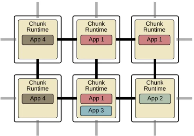
Figure 3.1: Overview of the Chunk Platform. Each substrate node runs a Chunk Runtime, which uses the substrate’s local network connections to communicate with other Chunk Runtimes.

Local and Distributed Modern computing substrates are composed of independent com-ponents for which local interactions are far more efficient than long-range interactions. As these substrates scale in size and complexity, it becomes more difficult to build and maintain centralized global databases about the state of the system and its compo-nents.

Elastic Modern computing substrates are elastic and require balancing the use of extra computing elements with the costs, either in power or dollars, of using those elements. There are two parts to making an elastic computing system: expanding the amount of hardware a computation uses as the computation grows and shrinking the amount of hardware used as the computation finishes off.

The Chunk Platform embraces these common properties with two high-level design princi-ples. First, the Chunk Platform shuns global routing and global shared memory and instead exploits local neighborhoods of connections between nodes to distribute the universe of chunks among the locally-available resources on each node. This design decision leads to a Chunk Platform architecture centered around a network protocol that leverages those local connections and resources to effect global changes in the universe of chunks. Second, since reclaiming resources in a distributed system can be complex and error-prone, yet is necessary to cost-effectively use modern computing substrates, the Chunk Platform provides distributed garbage collection to reclaim chunks as computations wane.

(47)

Chunk Stream

SCVM

JSLite Photo_Boss Tasklets

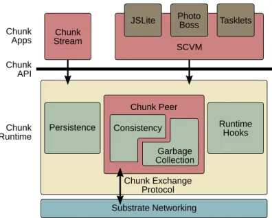
Chunk API Chunk Apps Substrate Networking Chunk Runtime Runtime Hooks Garbage Collection Consistency Persistence Chunk Exchange Protocol Chunk Peer

Figure 3.2: Architectural diagram of the Chunk Platform running on a single substrate node.

Figure 3.1 illustrates the overall architecture of the Chunk Platform as it fits into a generic modern computing substrate. Each node in the substrate hosts a Chunk Runtime, which, in turn, hosts one or more applications that use chunks. The Chunk Runtime on each node lets its applications create, read, and modify chunks distributed among the nodes. Chunk Runtimes communicate with each other using the Chunk Exchange Protocol. The Chunk Exchange Protocol manages where chunk copies are located, how copies are updated with modifications, and how allocated chunks are reclaimed when no applications need them anymore. Note that while the nodes and Chunk Runtimes in Figure 3.1 may look identical, the implementations of the Chunk Runtimes on each node may be different; the Chunk Platform only requires all Chunk Runtimes to use chunks of the same size and to communicate using compatible versions of the Chunk Exchange Protocol.

Figure 3.2 shows the software architecture of the Chunk Platform running on a single node. The Chunk Platform provides a Chunk API that serves as a concrete interface to the Chunk Model. Applications use the Chunk API to create, read, and modify chunks. In turn, the Chunk Runtime implements those API calls by using the Chunk Exchange Protocol to redistribute chunk copies so as to satisfy the contracts of the calls. In addition to the Chunk API, the Chunk Runtime provides generic system services for using chunks. These services include persistence of chunks, optimization libraries, as well as the Chunk Peer,

(48)

which handles the Chunk Exchange Protocol. The Chunk Runtime is implemented on top of a substrate-specific networking layer, e.g., a layer using WebSockets [34] in the cloud, or on-chip networking instructions in massively multi-core processors.

The rest of this chapter details the particular choices for the Chunk API and the imple-mentation of the Chunk Runtime that comprise the Chunk Platform.

3.2 The Chunk API and Memory Model

The Chunk API is the application-level expression of the Chunk Model: it provides a window into the shared universe of chunks and provides mechanisms for manipulating the chunk graph. The particular Chunk API we chose for the Chunk Runtime balances the needs of applications—providing standard mechanisms to create, modify, and find chunks—with the needs of the Chunk Platform—namely knowing when applications are actively using chunks or actively modifying chunks, in addition to determining when chunks are no longer needed by applications. As shown in Table 3.1, the API is divided into four groups of functions: functions to create chunks, functions to read chunks, functions to modify chunks, and system-level functions used internally within the Chunk Runtime to manage chunk references across the Chunk Platform’s network of nodes.

3.2.1 API Usage

Chunks are created in two steps. First, applications callnew_chunk()to create an nameless, ephemeral chunk. To insert the chunk into the Chunk Platform, the application calls

insert(chunk), which names the chunk with a chunk ID and persists it within local storage of the Chunk Runtime. Chunk IDs form the core linking abstraction for the Chunk Platform; once a chunk has been assigned an ID, that chunk can be used as a link target of other chunks as well as a parameter to the Chunk API. If an application attempts to de-reference an invalid chunk ID, the Chunk Runtime will raise an exception, much like de-referencing an invalid address may cause a virtual memory system to cause a general protection fault.

For example, to create the data structure in Figure 2.2, we first callnew_chunk()to create the image chunk. After filling the chunk with image data, we callinsert()to persist the chunk to the store;insert()returns an identifier (#73) to use to refer to the chunk. Next, we callnew_chunk()a second time to create the text chunk. After filling the first seven slots with

(49)

Chunk Creation

new_chunk()returnsa chunk

Create a new, unnamed, uninitialized chunk.

insert(chunk)returnsID

Insert chunkinto the store and return the chunk’s identifier. The calling process will hold Modify privileges on the chunk.

Read API

get(id)returnsa chunk

Block until obtaining Read privileges on the chunk, then return the chunk.

wait(id, status)returnsvoid

Block until the specified chunk has changed from the given status.

free(id)returnsvoid

Release all privileges held for the chunk. Modify API

lock(id)returnsa chunk

Block until obtaining Modify privileges on the chunk, then return the chunk.

modify(id, chunk)returnsvoid

Modify the chunk associated with the chunk identifier so that it has the contents ofchunk. Requires Modify privileges.

unlock(chunk_id)returnsvoid

Downgrade Modify privileges to Read privileges. Internal API

bootstrap(id, from)returnsvoid

Bootstrap reference to a chunk held on another node in the network.

gc_root_add(id)returnsvoid

Add a chunk to the garbage collector’s set of live chunks.

gc_root_remove(id)returnsvoid

Remove a chunk to the garbage collector’s set of live chunks. Table 3.1: Chunk API exposed by the Chunk Runtime.

Computing with Chunks