Object grammars and random generation

(1)

HAL Id: hal-00958902

https://hal.inria.fr/hal-00958902

Submitted on 13 Mar 2014

HAL is a multi-disciplinary open access

archive for the deposit and dissemination of sci-entific research documents, whether they are pub-lished or not. The documents may come from teaching and research institutions in France or abroad, or from public or private research centers.

L’archive ouverte pluridisciplinaire HAL, est destinée au dépôt et à la diffusion de documents scientifiques de niveau recherche, publiés ou non, émanant des établissements d’enseignement et de recherche français ou étrangers, des laboratoires publics ou privés.

Object grammars and random generation

I. Dutour, Jean-Marc Fedou

To cite this version:

I. Dutour, Jean-Marc Fedou. Object grammars and random generation. Discrete Mathematics and Theoretical Computer Science, DMTCS, 1998, 2, pp.49-63. �hal-00958902�

(2)

Object grammars and random generation

I. Dutour and J. M. F´edou

✁

✂

LaBRI, Universit´e Bordeaux I, 351 cours de la Lib´eration, 33405 Talence Cedex, France E-mail:dutour@labri.u-bordeaux.fr

✄

I3S-ESSI, Universit´e de Nice, 650 Route des Colles, B.P. 145, 06903 Sophia-Antipolis Cedex, France E-mail:fedou@unice.fr

This paper presents a new systematic approach for the uniform random generation of combinatorial objects. The method is based on the notion of object grammars which give recursive descriptions of objects and generalize context-free grammars. The application of particular valuations to these grammars leads to enumeration and random genera-tion of objects according to non algebraic parameters.

Keywords: Uniform random generation, object grammars,☎ -equations

1 Introduction

An object grammar defines classes of objects by means of terminal objects and certain types of operations applied to the objects. It is most often described with pictures. For instance, the standard decomposition of complete binary trees is an object grammar (Figure 1). The formalism given here for object gram-mars [6, 7] generalizes the one for context-free gramgram-mars. An important application of these gramgram-mars is a systematic approach for the specification of bijections between sets of combinatorial objects (see [7]).

The paper outlines another important application of the object grammars: a systematic method for gen-erating combinatorial objects uniformly at random. The work lies in the recursive method framework; this method is to generate recursively random objects by endowing a recurrence formula with a probabilistic interpretation. This generation process has been first formalized by Nijenhuis and Wilf [11, 14, 15]. They have a general approach. They base the recursive procedure on an acyclic directed rooted graph with a terminal vertex and numbered edges, graph which depends on the family of objects. The recursive method has been also formalized by Hickey and Cohen in the special case of context-free languages [10], and by Greene within the framework of the labelled formal languages [9].

Recently, Flajolet, Zimmermann and Van Cutsem have given a systematic approach for this method with specifications of structures by grammars involving set, sequence and cycle constructions [8]. The methods that they have examined enable to start from any hight level specification of decomposable class and compile automatically procedures that solve the corresponding random generation problem. They have presented two closely related groups of methods: the sequential algorithms (linear search) which have worst case time complexity ✆✞✝✠✟☛✡✌☞, when applied to objects of size ✟ , and the boustrophedonic

algorithms (bidirectional fashion) which have worst case time complexity✆✞✝✠✟✎✍✑✏✓✒✔✟☛☞.

The present work is a continuation of the research of these authors. It is a systematization of the recursive method based on the object grammars. It then extends the field of structures which can be

1365–8050 c✕

(3)

Fig. 1: Complete binary trees.

generated using such method. Another important contribution of this work is to consider the random generation of objects according to several parameters simultaneously, and to consider not only algebraic parameters (i.e. that lead to algebraic generating functions), but also parameters that lead to generating functions satisfying✖ -equations. The other methods have rarely dealed with these latest parameters.

In section 2, we review the necessary definitions for object grammars. We then provide in section 3 the notion of✖ -linear valuations. They formalize the behaviour (on objects defined by an object grammar) of parameters that lead automatically to✖ -equations satisfied by the corresponding generating functions.

Section 4 introduces our systematic random generation method. Given an unambigous object grammar and a corresponding✖ -linear valuation, it allows to construct automatically the enumeration and uniform generation procedures according to the valuation. These procedures use sequential algorithms and have worst case time complexity✆✗✝✠✘✚✙✛✝✠✘✢✜✣✙✠☞✛☞ , when applied to objects of valuation✤✦✥✓✖★✧, assuming the enumer-ation tables have been computed once for all in✆✗✝✠✘✩✡✪✙✠✡★☞ time (see [6] for the general case of valuation). If one only considers an algebraic parameter (✤✩✥ ), the complexity is the same as in [8], and the boustro-phedonic search can be used. Note that, as in [8], the complexity is related to the number of arithmetic operations, unit cost is taken for the manipulation of a large integer.

The path taken here is eminently praticable and the method has been implemented in the Maple lan-guage (package named qAlGO). Section 5 gives some results obtained with this program concerning the uniform random generation of convex polyominoes according to the area and planar trees according to the internal path length. The package CombStruct, written by P. Zimmermann, cannot study these objects and this type of parameter. The packages qAlGO and CombStruct complement each others. In section 6, we finish by discussing some ideas and directions of research.

2 Object Grammars

Let✫ be a family of sets of objects. An object operation (in✫ ) is a mapping✬✮✭✦✯✱✰✳✲✮✴✵✴★✴✚✲✶✯ ✥✸✷✺✹

✯ , where✯✼✻✮✫ and✯✾✽✿✻❀✫ for❁ in❂

✓❃

✘❅❄. It describes the way of building an object of ✯ from✘ objects belonging to✯✱✰ ❃ ✴✵✴★✴ ❃ ✯ ✥ , respectively. The domain of✬ is✯❆✰❇✲✶✴★✴★✴✓✲❈✯ ✥

, denoted by❉✚❊●❋✶✝✠✬☛☞, the codomain is✯ , denoted by❍✌❊●❉✚❊●❋✶✝■✬☛☞ and the image is denoted by❏✓❋❑✝✠✬☛☞. The❁-th projection✯✿✽ of❉✚❊●❋✶✝■✬☛☞ is called a component of✬ .

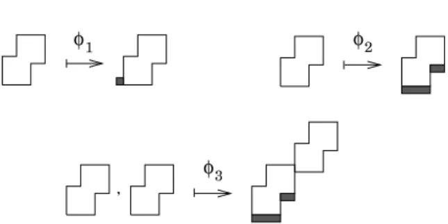
Example 2.1 . A parallelogram polyomino can be defined as the surface lying between two North-East paths that are disjoint, except at their common ending points (see Figure 2) [5]. Let✯✔▲✪▲ be the set of parallelogram polyominoes.

The mappings ✬▼✰ , ✬

✡

and ✬❖◆ illustrated in Figure 3 are object operations in ✫◗P❙❘❚✯ ▲✪▲✚❯ . The operations✬ ✰ and✬

✡

are operations of arity (✯✔▲✪▲ ✷✺✹

✯✔▲✪▲ ). The operation✬ ✰ glues a new cell at the left of the lowest cell of the first column of a polyomino. The operation ✬

✡

adds a new cell at the bottom of each column of a polyomino. The operation ✬ ◆ is an operation of arity

✁

(✯✔▲✪▲✗✲✶✯✔▲✪▲ ✷✺✹

(4)

Fig. 2: A parallelogram polyomino.

φ❱

φ❲

φ❳

,

Fig. 3: Object operations on parallelogram polyominoes.

them by one cell: the top-cell of the last column of the first polyomino facing the bottom-cell of the first column of the second.

Definition 2.1 An object grammar is a❨ -tuple❩❬✫

❃✛❭❈❃❫❪❈❃✪❴❛❵

where:

✫ P❜❘❚✯

✽

❯

✽■❝●❞ is a finite family of sets of objects. (I is a finite subset of IN).

❭

P❜❘✵❡❖❢▼❣ ❯

✽■❝●❞ is a finite family of finite subsets of sets of

✫ ,❡❖❢✢❣✾❤✐✯ ✽,

whose elements are called terminal objects.

❪

is a set of object operations ✬ in✫ .

S is a fixed set of✫ called the axiom of the grammar. The dimension of an object grammar is the cardinality of✫ .

Remark. Sometimes a❥ -tuple❩❦✫

❃✛❭❈❃❧❪♠❵

is called also object grammar. The axiom is chosen later in ✫ .

In the following, the terms grammar and operation will often be used for object grammar and object operation respectively.

The construction of an object can be described by its derivation tree : internal nodes are labelled with object operations and leaves with terminal objects. These derivation trees are comparable to the abstract trees within the theory of Compiling.

Let♥♦P✣❩♠✫

❃✛❭✗❃❫❪♣❵

be an object grammar and ✯q✻❦✫ a set of objects. An object ❊ is said to be

generated in♥ by✯ , if there is a derivation tree of♥ on✯ (i.e. the codomain of the label of the root is ✯ ) whose evaluation is❊ .

The set of objects generated by✯ in♥ is denoted byrts✿✝✠✯t☞. If

❴

in✫ is chosen as the axiom of♥ , then rts✉✝

❴

(5)

φ✈ φ✇

φ✇

φ①

φ① φ✇

Fig. 4: A derivation tree in②

✄

.

Example 2.2 . Let’s note③ the one-cell polyomino. Here are two examples of object grammars: ♥④✰⑤P ❩⑥❘●✯ ▲✪▲✩❯ ❃ ❘✓❘✓③ ❯✓❯ ❃ ❘●✬▼✰ ❃ ✬ ✡ ❯ ❃ ✯ ▲✪▲ ❵ and ♥ ✡ P ❩⑥❘●✯ ▲✪▲✩❯ ❃ ❘✓❘✓③ ❯✓❯ ❃ ❘●✬▼✰ ❃ ✬ ✡ ❃ ✬❖◆ ❯ ❃ ✯ ▲⑦▲ ❵ .

The parallelogram polyomino of Figure 2 belongs tor s▼⑧ ✝✠✯ ▲✪▲ ☞, its derivation tree in♥

✡

is given in Figure 4. The setr s✢⑧ ✝✠✯ ▲✪▲ ☞ is the set of parallelogram polyominoes.

The setr s⑩⑨ ✝✠✯ ▲✪▲ ☞ is the set of Ferrers diagrams; it is a proper subset of parallelogram polyominoes. By analogy to context-free grammars, an object grammar♥ is unambiguous if every object inr

s

✝

❴

☞

has exactly one derivation tree. Unambiguity is an important property for building bijections.

One can also define several normal forms for object grammars: reduced, 1-2 or complete. The reduced and 1-2 forms extend usual normal forms of context-free grammars: the reduced and Chomsky normal form. A grammar is said to be reduced if every set of objects ✯ in✫ is accessible from the axiom and rts✉✝✠✯t☞❷❶P❹❸ ; it is said to be in 1-2 form if all its operations are of arity or

✁

. The complete form is specific for object grammars. A grammar is said to be complete ifrts✾✝■✯t☞✔P❺✯ for every set of objects✯ in✫ (generallyr✣s✾✝✠✯t☞✿❻⑥✯ ). For example, the grammar♥

✡

previously defined is complete while♥ ✰ is not. The details on transformations of object grammars into normal forms are given in [6].

Another Definition

A complete, unambiguous object grammar♥⑥P✣❩❼✫

❃✛❭✗❃❫❪❈❃✪❴✮❵

can be described as a system of equations

❽

involving sets of objects, terminal objects and object operations, or as a system of graphic equations. The equations describe the decomposition of a set of objects into a disjoint union of terminal objects and images of operations: ❽ P ❾ ❿➀ ✯✿✽✢P ➁ ➂ ❣❝✵➃➅➄ ❣✓➆ ✽♠✜ ➁ ➇➉➈✛➊✪➈❫➋✎➌➎➍●➏➑➐ ❢ ❣ ✬➒✝■✯✾✽⑨■➓➔ ❃ ✴✵✴★✴ ❃ ✯✿✽➣→ ➓➔ ☞✓↔↕ ➙ ✽ ➐ ✰✪➛➝➜➝➜➝➜➛➞ .

For example, the equation for the grammar♥

✡

generating parallelogram polyominoes previously defined is ✯ ▲⑦▲ P❺③❀✜❬✬▼✰❚✝■✯ ▲✪▲ ☞☛✜➟✬ ✡ ✝✠✯ ▲✪▲ ☞☛✜❼✬❖◆✓✝✠✯ ▲⑦▲ ❃ ✯ ▲✪▲ ☞➠✴

(6)

Fig. 5: Schematic object grammar for parallelogram polyominoes.

Expanded 1-2 form

The automatic method of random generation presented in the paper is based on the expanded 1-2 form of object grammars.

An object grammar♥➡P✣❩❦✫

❃✛❭✗❃❫❪➢❵

is called in expanded 1-2 form if, for every✯ in✫ , the equation that defines it has one of the forms

✯➡P ➆ ; ✯➡P❺✯ ✰ ✜❼✯ ✡ ; ✯➡P❺✬➒✝✠✯ ✰ ☞; ✯➡P❺✬➒✝✠✯ ✰ ❃ ✯ ✡ ☞.

Proposition 2.2 Every object grammar has an equivalent expanded 1-2 form.

Proof. To transform an object grammar into an expanded 1-2 form, it suffices to change all the sums and domains of the object operations having arity❵❦✁

by adding sets of objects and identity object operations of arity✁

. Thus, the equation✯➡P❺✬➒✝✠✯❆✰

❃

✴★✴✵✴

❃

✯

✥

☞ is replaced by the set of equations ✯➡P❺✬❖❢ ⑨ ✝✠✯ ✰ ❃✪➤ ❢ ⑧ ☞, ➤ ❢ ⑧ P❺✬❖❢ ⑧ ✝✠✯ ✡ ❃✪➤ ❢☛➥✌☞, . . . , ➤ ❢➦→➨➧ ⑨ P❦✬❖❢☛→✪➧ ⑨ ✝✠✯ ✥❅➩ ✰ ❃ ✯ ✥ ☞. ③

In the following, we will often use the term 1-2 form for expanded 1-2 form.

3 Enumeration

Let➫ be a ring and➭♣P➯❘❚✤➲✰

❃

✴★✴✵✴

❃

✤✩➞ ❯ a set of variables. Then➫✮❂➭✸❄ (resp. ➫✮❂✑❂➭✸❄➎❄) denotes the set of

polynomials (resp. formal power series) in the variables✤➲✰

❃

✴✵✴★✴

❃

✤✩➞ having coefficients in➫ . Given a set of objects✯ , an object valuation (on✯ ) is a mapping➳ ❢ ✭✓✯

✷➦✹ ➫✮❂➭✸❄ satisfying ➵ ✝✠✘✩✰ ❃ ✴★✴★✴ ❃ ✘❅➞➅☞✉✻ IN ➞✢➸ ❘ ➆ ✻✶✯t➺✣❩➻✤➲✰ ✥ ⑨ ✴★✴✵✴✛✤✦➞ ✥●➼ ❃ ➳ ❢ ✝ ➆ ☞ ❵t❃ ❶P❦➽ ❯ is finite. Consequently, the generating function associated with✯ ,

➁

➂

❝ ❢ ➳➅❢✳✝

➆

☞ , is a formal power series which lies in➫✮❂✑❂➭✸❄✑❄. It will be denoted by➳ ❢ ✝■✯t☞.

Theorem 3.1 Let♥❺P✣❩❦✫

❃✛❭④❃❧❪✐❵

be a complete, unambiguous object grammar, and➾✗P➡❘❅➳➅❢❼✭✚✯ ✷✺✹ ➫✮❂➭✸❄

❃

✯❺✻✶✫ ❯ a set of object valuations. For all✯ in✫ , from its equation in♥

✯ P ➁ ➂ ❝★➃ ➄ ➆ ✜ ➁ ➇➉➈➉➊✪➈❧➋✳➌➎➍●➏➚➐ ❢ ✬➒✝✠✯ ✽⑨■➓➔ ❃ ✴✵✴★✴ ❃ ✯ ✽→ ➓➔ ☞ , (1)

one can directly obtain the following equation:

➳ ❢ ✝✠✯t☞➪P ➳ ❢ ✝➚❡ ❢ ☞♠✜ ➁ ➇➉➈➉➊✪➈❧➋✳➌➎➍●➏➚➐ ❢ ➳ ❢ ✝■✬➒✝✠✯✿✽⑨■➓➔ ❃ ✴✵✴★✴ ❃ ✯✿✽➣→ ➓➔ ☞➉☞ . (2)

(7)

Proof. The object grammar♥ is unambiguous and complete, given equation (1). Equation (2) is obvious, since we have disjoint unions.

③

The objective is to obtain a system of equations for the generating functions of the sets of the grammar. Then, one has to express ➳

❢ ✝✠✬➒✝■✯✾✽ ⑨✠➓➔ ❃ ✴★✴✵✴ ❃ ✯✾✽➑→ ➓➔ ☞✛☞ in terms of ➳ ❢ ❣ ⑨■➓➔ ✝■✯✾✽ ⑨■➓➔ ☞, . . . , ➳ ❢ ❣ → ➓➔ ✝✠✯✿✽➣→ ➓➔ ☞ . This depends on the nature of object valuations considered.

Example 3.1 . Let✯ ▲✪▲ be the set of parallelogram polyominoes and consider the following valuation: ➳✚➶✢➹➘✭♦✯✔▲✪▲ ✷☛✹ IN❂➝✤ ❃ ✖➠❄ ➆ ➴ ✷☛✹ ✤ ➶ ✽ ➊✛➷✠➬➮➌➎➂➉➏ ✖ ➹✪➱ ➂ ➹ ➌➎➂✛➏

It is well-known that the generating function ➳➅➶✢➹✚✝■✯✔▲✪▲✚☞, denoted here by ✃★➶✢➹✚✝■✤

❃

✖●☞ , satisfies the ✖ -equation (see for example [3])

✃★➶✢➹✚✝■✤ ❃ ✖●☞➒P⑥✤❖✖❇✜❼✤❖✖●✃★➶✢➹✓✝■✤ ❃ ✖●☞☛✜❼✃★➶✢➹✚✝✠✤❖✖ ❃ ✖●☞☛✜❬✃★➶✢➹✚✝✠✤❖✖ ❃ ✖●☞✛✃★➶✢➹✚✝✠✤ ❃ ✖●☞ . The object valuation ➳

➶✢➹ is called

✖ -linear. The general definition of such a valuation is detailed below.

❐

-linear Object Valuations

Let➭❒P❜❘❚✤➲✰ ❃ ✴✵✴★✴ ❃ ✤✩➞ ❯ and❮➡P❜❘❚✖➮✰ ❃ ✴★✴✵✴ ❃

✖ ➱➮❯ be two disjoint sets of variables.

Notations. ✤ denotes the✟ -tuple ✝✠✤

✰ ❃ ✴★✴★✴ ❃ ✤ ➞

☞ and✖ the ❰ -tuple ✝✠✖

✰ ❃ ✴✵✴★✴ ❃ ✖➠➱✌☞ . IfÏ is a matrix having coefficients in IN (Ï❺P➡✝✠Ð ✽➝Ñ ☞, ✎Ò ❁ Ò ✟ , ✎Ò❬ÓÔÒ ❰ ), then Õ ✤❖✖★Ö❀P➡✝■✤ ✰ ✖ ✰ ➹★⑨■⑨ ✴✵✴★✴➉✖➠➱ ➹★⑨■× ❃ ✴✵✴★✴ ❃ ✤ ➞ ✖ ✰ ➹ ➼ ⑨ ✴★✴✵✴❫✖➠➱ ➹ ➼ × ☞, Õ for✃✢✝■✤ ❃ ✖●☞✉✻✶➫✮❂✑❂➭ ❃ ❮✎❄✑❄,✃▼✝✠✤ ❃ ✖●☞✵ØÙ✓Ú✎Ù✵Û✪ÜÝP❺✃▼✝✠✤❖✖ Ö ❃ ✖●☞. Let ✯ ❃ ✯ ✰ ❃ ✴★✴✵✴ ❃ ✯ ✥ be sets of objects, ➳✚❢ ❃ ➳➅❢ ⑨ ❃ ✴★✴✵✴ ❃ ➳✚❢☛→ object valuations on ✯ ❃ ✯ ✰ ❃ ✴★✴★✴ ❃ ✯ ✥ respec-tively, and✬ an object operation with❍➠❊●❉➅❊●❋❑✝✠✬☛☞❅PÝ✯ and❉➅❊●❋❑✝✠✬☛☞✔P❺✯ ✰ ✲✮✴★✴✵✴❅✲✶✯

✥

. ➳✚❢ is called✖ -linear with respect to✬ if it exists a polynomial Þ

➍ in ➫✮❂➭ ❃ ❮✎❄ and matricesÏ ✽ ➍ for ❁▼✻ß❂ ✓❃ ✘❅❄ such that ➳➅❢✎✝✠✬➒✝ ➆ ✰ ❃ ✴★✴✵✴ ❃ ➆ ✥ ☞✛☞✔P❺Þ ➍ ✥ à ✽ ➐ ✰ ➳✚❢✢❣✪✝ ➆ ✽ ☞★Ø Ù✓Ú✳Ù★Û Ü ❣ ➔ , for every ✝ ➆ ✰ ❃ ✴★✴✵✴ ❃ ➆ ✥ ☞á✻â❉✚❊●❋✶✝■✬☛☞✌✴ If✬ is injective, then ➳ ❢ ✝✠✬➒✝■✯❆✰ ❃ ✴✵✴★✴ ❃ ✯ ✥ ☞✛☞✔P❺Þ ➍ ✥ à ✽ ➐ ✰ ➳ ❢ ❣✪✝✠✯✿✽✠☞✵Ø Ù❅Ú✳Ù✵ÛÜ ❣ ➔ ✴

Corollary 3.2 If all the object valuations of➾ are✖ -linear, equation (2) of Theorem 3.1 becomes:

➳ ❢ ✝✠✯t☞ãP ➳ ❢ ✝➑❡ ❢ ☞♠✜ ➁ ➇➉➈✛➊⑦➈❧➋✳➌✑➍●➏➑➐ ❢ Þ ➍ ✽➑→ ➓➔ à ✽ ➐ ✽⑨✠➓➔ ➳ ❢ ❣⑦✝■✯✾✽✠☞★Ø Ù❅Ú✳Ù★Û Ü ❣ ➔ . (3)

(8)

Example 3.2 . The object valuation➳ ➶✢➹ is✖ -linear with respect to the object operations✬▼✰ ,✬

✡

and✬❖◆ . Then the equation

➳ ➶✢➹ ✝■✯ ▲✪▲ ☞➒P➡➳ ➶✢➹ ✝❫③✾☞✢✜➻➳ ➶✢➹ ✝■✬▼✰❚✝■✯ ▲✪▲ ☞✛☞☛✜ä➳ ➶✢➹ ✝■✬

✡

✝✠✯ ▲⑦▲ ☞✛☞☛✜ä➳ ➶✢➹ ✝■✬❖◆✓✝✠✯ ▲⑦▲

❃

✯ ▲✪▲ ☞✛☞

becomes the✖ -equation seen before (✃★➶✢➹✚✝✠✤

❃ ✖●☞➒P❜➳➅➶✢➹✚✝■✯✔▲✪▲➅☞ ) ✃★➶✢➹✚✝■✤ ❃ ✖●☞➒P⑥✤❖✖❇✜❼✤❖✖●✃★➶✢➹✓✝■✤ ❃ ✖●☞☛✜❼✃★➶✢➹✚✝✠✤❖✖ ❃ ✖●☞☛✜❬✃★➶✢➹✚✝✠✤❖✖ ❃ ✖●☞✛✃★➶✢➹✚✝✠✤ ❃ ✖●☞ .

Special Case: Linear Object Valuations

The linear object valuations are✖ -linear object valuations such that, for every object operation✬ and all i,Ï✳✽

➍

P➢✝✠➽✓☞ . These linear valuations are exactly in the DSV methodology framework [2, 13], they yield algebraic generating functions (see [6]).

Object Valuations and 1-2 form

The proof of Proposition 2.2 has shown how to reduce object grammars in 1-2 form. The✖ -linear object valuations are very well preserved through this transformation.

Proposition 3.3 If➾ is a set of✖ -linear object valuations associated with an object grammar, it is possible

to construct an equivalent set of object valuations associated with its 1-2 form. Proof. Recall that an equation✯⑥P❺✬➒✝✠✯ ✰

❃

✴✵✴★✴

❃

✯

✥

☞ in the grammar is replaced by the set of equations ✯➡P❺✬❖❢ ⑨ ✝✠✯ ✰ ❃✪➤ ❢ ⑧ ☞, ➤ ❢ ⑧ P❺✬❖❢ ⑧ ✝✠✯ ✡ ❃✪➤ ❢☛➥✌☞, . . . , ➤ ❢➦→➨➧ ⑨ P❦✬❖❢☛→✪➧ ⑨ ✝✠✯ ✥❅➩ ✰ ❃ ✯ ✥ ☞. Concerning the object valuations, if we have

➳✚❢✳✝■✬➒✝✠✯ ✰ ❃ ✴✵✴★✴ ❃ ✯ ✥ ☞✛☞✔P⑥Þ ➍ ✥ à ✽ ➐ ✰ ➳➅❢▼❣⑦✝■✯ ✽ ☞✵Ø Ù✓Ú✎Ù✵Û Ü ➔ ❣ ❃ then we define ❾å å å å å å å å å å ❿ å å å å å å å å å å ➀ ➳✚❢✳✝✠✬❖❢ ⑨ ✝✠✯ ✰ ❃⑦➤ ❢ ⑧ ☞➉☞ P Þ ➍ ➳✚❢ ⑨ ✝✠✯ ✰ ☞●Ø Ù❅Ú✳Ù✵Û Ü ➔ ⑨ ✴✚➳➅æ ➄ ⑧ ✝ ➤ ❢ ⑧ ☞ ✃❖❊●❰❼❁☛P ✁ ✴★✴★✴ç✘ ✷ ✁✦❃ ➳ æ ➄ ❣ ✝ ➤ ❢ ❣❫☞ P ➳ æ ➄ ❣ ✝■✬ ❢ ❣➉✝■✯✾✽ ❃⑦➤ ❢ ❣è ⑨ ☞➉☞ P ➳ ❢ ❣⑦✝■✯✾✽❫☞✵Ø Ù❅Ú✳Ù✵Û Ü ➔ ❣ ✴✚➳ æ ➄ ❣è ⑨ ✝ ➤ ❢ ❣è ⑨ ☞ ➳ æ ➄ →✪➧ ⑨ ✝ ➤ ❢ →✪➧ ⑨ ☞ P ➳ æ ➄ →➨➧ ⑨ ✝■✬ ❢ →➨➧ ⑨ ✝✠✯ ✥✓➩ ✰ ❃ ✯ ✥ ☞➉☞ P ➳ ❢ →✪➧ ⑨ ✝■✯ ✥❅➩ ✰⑦☞➮é é Ù❅Ú✳Ù★Û Ü ➔ →✪➧ ⑨ ✴á➳ ❢ →✚✝■✯ ✥ ☞★Ø Ù❅Ú✳Ù★Û Ü ➔ →

(9)

4 Enumeration and Random Generation Procedures

Not all object grammars ♥ and possible corresponding sets of functions ➾ lead to random generation. The couples ✝✠♥

❃

➾✺☞ considered here are well-founded, i.e. each set of objects generates at least one ob-ject, and it generates a finite number of objects having the same valuation’s value (it is the definition of an object valuation). An algorithm performing this task is detailed in [6]. It is inspired by works of Zimmermann [16].

In the following, the study is limited to the case of✖ -linear object valuations having values in the set of monomials denoted by ê✶❊●✟➒❂➭

❃

❮✎❄. Moreover, ➭ and❮ contain only one variable: ➭ëPì❘●✤ ❯ and ❮⑥P❜❘❚✖ ❯ . The complete case is detailed in [6].

4.1 Enumeration Procedures

Let♥⑥P✣❩❼✫

❃✛❭❈❃❧❪✐❵

be an object grammar in expanded 1-2 form and➾✗P➡❘❅➳ ❢ ✭✓✯ ✷✺✹ ê❑❊●✟➒❂✤ ❃ ✖➠❄ ❃ ✯ä✻

✫ ❯ a set of✖ -linear valuations such that the couple✝✠♥

❃

➾✺☞ is well-founded. The generating function of a set of objects✯ is denoted by

➳✚❢✳✝■✯t☞✔P í ➁ î ➛ï ➐☛ð ❍✪❢✎✝✠➫ ❃✪ñ ☞▼✤ î ✖ ï ✴

Theorem 4.1 (i) The coefficients❍✪❢✳✝✠➫ ❃⑦ñ

☞ are given by the following formulas :

Õ ✯➡P ➆ , then if ➳ ❢ ✝ ➆ ☞✔P❺✤ î ✖ ï then ❍ ❢ ✝✠➫ ❃⑦ñ ☞➒P else ➽ ❃ Õ ✯➡P❺✯❆✰✢✜❼✯ ✡ , then ❍ ❢ ✝■➫ ❃✪ñ ☞✔P❺❍ ❢▼⑨ ✝✠➫ ❃⑦ñ ☞☛✜❼❍ ❢☛⑧ ✝■➫ ❃✪ñ ☞ ❃ Õ ✯➡P❺✬➒✝✠✯❆✰✪☞ with➳ ❢ ✝✠✬➒✝✠✯✱✰➨☞✛☞✔P❦✤✩✥✵ò✌✖★✧óò➲➳ ❢▼⑨ ✝✠✯❆✰✪☞✵ØÙ✓Ú✎Ù✵Û✪ô ⑨ , then ❍✪❢✳✝✠➫ ❃⑦ñ ☞õP❺❍✪❢ ⑨ ✝■➫ ✷ ✘ ð ❃✪ñ ✷ ✙ ð ✷ ✝✠➫ ✷ ✘ ð ☞➠✴➝Ð ✰ ☞ ❃ Õ ✯➡P❺✬➒✝✠✯❆✰ ❃ ✯ ✡ ☞ with➳ ❢ ✝✠✬➒✝■✯❆✰ ❃ ✯ ✡ ☞✛☞✔P❺✤✦✥ ò ✖★✧ ò ➳ ❢▼⑨ ✝✠✯❆✰✌☞✵ØÙ✓Ú✎Ù✵Û ô ⑨ ➳ ❢☛⑧ ✝✠✯ ✡ ☞★ØÙ❅Ú✳Ù★Ûô ⑧ , then ❍✪❢✳✝■➫ ❃✪ñ ☞➒P î ➁ ✽ ➐☛ð ï ➁ Ñ ➐☛ð ❍✪❢ ⑨ ✝■❁ ❃❧Ó ☞✌✴➝❍✪❢ ⑧ ✝✠➫ ✷ ✘ ð ✷ ❁ ❃⑦ñ ✷ ✙ ð ✷ ❁➉✴➝Ð ✰ ✷ ✝✠➫ ✷ ✘ ð ✷ ❁■☞✌✴➝Ð ✡ ✷ Ó ☞✌✴

(ii) The computation of all the coefficients up to the value✤✩✥✓✖★✧ needs✆✗✝✠✘✩✡✌✙✠✡★☞ arithmetic operations.

(10)

With each set of objects of the grammar is associated a procedure having parameters and , and generating (uniformly at random) an object of✯ having the valuation✤✩✥✓✖★✧. More precisely, this procedure constructs the derivation tree in the grammar. It depends on the form of the equation which defines✯ in the object grammar:

Õ

✯➡P

➆

. The procedureö ❢ is trivial : ö✓❢❦✭➝P Proc(k,l) If➳✚❢÷✝ ➆ ☞✔P❺✤✩✥✓✖★✧ Then Return e End Proc Õ ✯✼P♠✯❆✰❇✜❦✯ ✡

. The procedureö ❢ must generate an object belonging either to ✯✱✰ or to✯

✡

. The probability that this object belongs to✯❆✰ is equal to❍ ❢✢⑨ ✝■✘

❃ ✙✠☞➉➺❅❍ ❢ ✝✠✘ ❃ ✙✠☞: ö ❢ ✭➝P Proc(k,l) ø := Uniform(❂➝➽ ❃★ ❄); Ifø ❩❦❍ ❢✢⑨ ✝✠✘ ❃ ✙✠☞➉➺❅❍ ❢ ✝■✘ ❃ ✙■☞ Then Returnö ❢▼⑨ ✝■✘ ❃ ✙■☞ Else Returnö ❢☛⑧ ✝✠✘ ❃ ✙✠☞ End Proc Õ ✯➡P❺✬➒✝✠✯❆✰✪☞, with➳ ❢ ✝■✬➒✝✠✯❆✰✪☞➉☞✔P❺✤✦✥★ò⑦✖★✧óò➲➳ ❢✢⑨ ✝✠✯✱✰⑦☞●ØÙ❅Ú✳Ù✵Û✪ô

⑨ . Then the procedure

ö

❢ is very simple. It returns an object of✯ obtained by✬ from an object of✯❆✰ having the valuation✤✩✥❅➩✺✥✵ò✪✖★✧✑➩✺✧óò➠➩

➌ ✥✓➩❖✥✵ò ➏ ➜➹★⑨ : ö ❢ ✭➝P Proc(k,l) ✘✦✘ :=✘ ✷ ✘ ð ; ✙➑✙ :=✙ ✷ ✙ ð ; Return✬➒✝❖ö✓❢ ⑨ ✝■✘✦✘ ❃ ✙➑✙ ✷ ✘✩✘☛✴➝Ð ✰ ☞õ☞ End Proc Õ ✯ùP♣✬➒✝✠✯✱✰ ❃ ✯ ✡ ☞, with ➳ ❢ ✝✠✬➒✝■✯❆✰ ❃ ✯ ✡ ☞➉☞úP♣✤✩✥ ò ✖★✧ò ➳ ❢▼⑨ ✝■✯❆✰⑦☞★ØÙ✓Ú✳Ù★Û ô ⑨ ➳ ❢☛⑧ ✝✠✯ ✡ ☞❚ØÙ✓Ú✎Ù✵Û ô ⑧ . The proce-dure ö ❢ must generate an object of ✯ obtained by ✬ from an object of ✯❆✰ and an object of

✯

✡

which respect the definition of the valuations. The probability for the object of ✯ ✰ having the valuation✤ î ✖ ï and those of✯ ✡

having the valuation✤✩✥✓➩❖✥✵ò✛➩

î ✖★✧✑➩❖✧óò✌➩ î ➜➹★⑨ ➩ ➌ ✥❅➩✺✥✵ò✛➩ î ➏ ➜➹✌⑧ ➩ ï is ❍✪❢ ⑨ ✝■➫ ❃✪ñ ☞✌✴➝❍✪❢ ⑧ ✝■✘ ✷ ✘ ð ✷ ➫ ❃ ✙ ✷ ✙ ð ✷ ➫✶✴➝Ð ✰ ✷ ✝■✘ ✷ ✘ ð ✷ ➫✶☞➠✴➝Ð ✡ ✷ ñ ☞✛➺✓❍✪❢❆✝✠✘ ❃

✙✠☞. The procedure is:

ö ❢ ✭➝P Proc(k,l) ✘✦✘ :=✘ ✷ ✘ ð ; ✙➑✙ :=✙ ✷ ✙ ð ; ❴ :=❍ ❢✢⑨ ✝✠➽ ❃ ➽✓☞➠✴➝❍ ❢➦⑧ ✝✠✘✦✘ ❃ ✙➑✙ ✷ ✘✩✘☛✴➝Ð ✡ ☞➉➺✓❍ ❢ ✝✠✘ ❃ ✙✠☞; ➫ :=➽ ; ø := Uniform(❂➝➽ ❃★ ❄); Whileø➡❵❦❴ Do ➫ :=➫♠✜ ; ❡ :=✙➑✙ ✷ ➫✶✴➝Ð ✰ ✷ ✝■✘✦✘ ✷ ➫❑☞✌✴➝Ð ✡ ; ñ :=➽ ;

(11)

Random generation algorithm: Input: a couple✝✠♥

❃

➾❖☞.

Output: procedures for generating the objects generated by♥ at random.

û

Transform♥ into 1-2 formP☛üù✝✠♥

ð ❃ ➾ ð ☞. û Verify that✝✠♥ ð ❃ ➾ ð

☞ is well-founded, else error.

û

For each set of objects✯ in♥

ð , create the enumeration procedure ❍ ❢ , then compute all the coefficients up to rank ✝■✘

❃

✙✠☞.

û

For each set of objects✯ in♥

ð , create the generation procedures ö ❢ as indicated above.

Fig. 6: A random generation procedure. Whileø❺❵➻❴ Andñ❬Ò ✙ Do ñ :=ñ ✜ ; ❴ :=❴ ✜ß❍✪❢ ⑨ ✝■✘ ❃ ✙✠☞✌✴➝❍✪❢ ⑧ ✝✠✘✩✘ ✷ ➫ ❃ ❡ ✷ ñ ☞✛➺✓❍✪❢✎✝✠✘ ❃ ✙✠☞; End While End While Return✬➒✝❖ö ❢▼⑨ ✝■✘ ❃ ✙■☞ ❃ ö ❢☛⑧ ✝✠✘✦✘ ✷ ➫ ❃ ❡ ✷ ñ ☞✔☞ End Proc

Theorem 4.2 The worst case time complexity of the generation procedures is of✆✗✝■✘✚✙➉✝■✘t✜✮✙✠☞✛☞ arithmetic

operations.

Proof. A random generation procedure consists in constructing recursively a derivation tree in♥ . This tree is binary because♥ is in 1-2 form. The size of the derivation tree of an object having the valuation ✤✦✥✓✖★✧ is proportional to✘Ô✜ä✙. The generation of a vertex of the tree has a maximal cost of✆✗✝■✘✚✙✠☞ (the loops of the procedure). Thus, the complexity of the generation of the derivation tree in the worst case is

✆✗✝✠✘ý✙➉✝✠✘❆✜✮✙■☞➉☞. ③

4.3 Algorithm for Uniform random generation

One can now describe an uniform random generation procedure for the objects of an object grammar according to a set of✖ -linear object valuations (Figure 6).

The obtained generation procedures give the derivation trees of objects in♥

ð, but not directly in ♥ . A simple transformation (linear cost in✆✗✝■✘t✜❬✙✠☞ ) gives the derivation trees in♥ . This postprocessing does not affect the conclusions of the complexity studies. Futhermore, at the expense of some programming effort, it can be effected ‘on the fly’.

5 Maple package qAlGO

The program qAlGO (in Maple language) implements the method developed in the previous sections. The package qAlGO builds automatically the enumeration and generation procedures from a unambiguous object grammar and a set of corresponding✖ -linear valuations (see the annex of [6] for syntax and use).

(12)

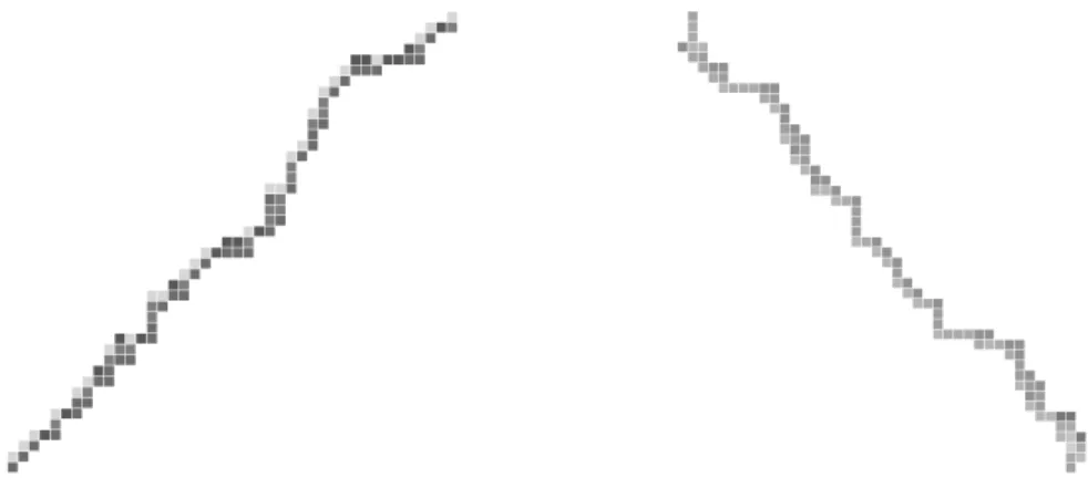
Fig. 7: A parallelogram polyomino of area 10.

The automatic nature of the software qAlGO gives a very useful tool which makes easy the experimental study of various statistics on combinatorial objects. In the following, we present relevant examples of random generation.

Convex Polyominoes According to the Area

Here is an example of experimental studies using qAlGO. It concerns the random generation, according to the area, of different classes of convex polyominoes: parallelogram polyominoes, convex directed polyominoes and convex polyominoes.

First, the example of parallelogram polyominoes. It suffices to give as input to qAlGO an object gram-mar that generates them and the corresponding object valuations: the gramgram-mar in Figure 5 and the valua-tion➳ ➶✢➹ defined in example 3.1. Thus one obtains the enumeration and the uniform generation according to the width (in✤ ) and the area (in✖ ).

> with(qalgo);

[compile, countgo, drawgo, drawgoall] # definition of the object grammar and valuations

> paralgo := { P = cell + phi1(P) + phi2(P) + phi3(P,P) }: > paralval := [[cell, 1, 1], [phi1, 1, 1, [0]],

[phi2, 0, 0, [1]], [phi3, 0, 0, [1, 0]]]: # construction of the procedures

> compile( paralgo, paralval, qlinear, Identity):

We are then able to generate these objects at random. More precisely, qAlGO returns the derivation tree of a random parallelogram polyomino. For example,

# generation of a polyomino having area 10 > drawgo( paralgo, paralval, qlinear, P, 10);

phi3(phi1(phi2(phi2(phi2(cellp)))), phi1(phi2(cellp)))

It then suffices to evaluate this derivation tree according to the object operations, and to write the poly-omino under a form understood by the interface XAnimal of CalICoþ [4, 12]; so we can visualize the polyomino Figure 7.

For the convex polyominoes, we use a much more complicated object grammar (of dimension 9 and with 34 object operations !), but the principle is exactly the same as before for the parallelogram polyomi-noes.ÿ

CalICo offers a software environment for manipulations and visualizations of combinatorial objects; it allows the communication

(13)

Fig. 8: Random parallelogram and convex polyominoes of perimeter✂✁✄✁ .

Fig. 9: Random parallelogram and convex polyominoes of area✂✁✄✁ .

Such experiments showed us how thin the random convex polyominoes according to the area is. Ac-cording to the perimeter, they look more thick. Examples of such polyominoes are given Figures 8 and 9. We also find out that convex polyominoes, random according to the area, have either a north-east, or north-west orientation (as Figure 9), with same probability one half.

To understand the thin look of such random polyominoes according to the area, we computed exper-imentally the average value of two parameters: the height of a column and the gluing number between two adjacent columns, which is the number of cells by which two adjacent columns are in contact. Af-ter generating ➽✓➽✓➽ convex polyominoes having area ➽✓➽ and ➽✓➽✓➽ parallelogram polyominoes having area✁

➽✓➽ , we obtain the following average values: ✁✩❃

❥✆☎ for the height of the columns, and ✓❃

❥✝☎ for the gluing number between two adjacent columns.

Remark. The result for the average height of a column (✁✦❃

❥✝☎ ) coincides exactly with what Bender [1] has obtained using asymptotic analysis methods.

The difference of between these two average parameters can be explained simply by noticing that this difference has for limit the quotient between the height and the width of the polyomino, which is by symmetry.

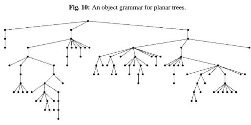
Planar Trees According to the Internal Path Length

(14)

Fig. 10: An object grammar for planar trees.

Fig. 11: A random planar tree of size 100.

length (ipl) of a tree is the sum of the distances of all its nodes from its root. The q-linear valuation

➳ ✽▲ ✧ ✭ ➆✳➴ ✷✺✹ ✤ ➞ ➈✛➊✪➂✟✞✪➌✑➂➉➏ ✖ ✽▲ ✧ ➌➎➂✛➏

leads to the following q-equation for the generating function ❡t✝■✤ ❃ ✖●☞➒P⑥✤✣✜ß❡t✝■✤✺✖ ❃ ✖●☞❫❡t✝■✤ ❃ ✖●☞ .

Setting✖ to , we obtain the linear valuation for the size of the trees (the number of nodes).

Using qAlGO with the above grammar and these two valuations, we are able to generate at random planar trees according to the size (see Figure 11), and also, according to the internal path length (see Figure 12). The latter have a remarkable look: they have a very small height.

6 Conclusions and Perspectives

The interest of our approach lies in its generality and simplicity. Time complexity are ‘computable’ and, at the same time, one gains access to the random generation of arbitrarily complex objects according to

(15)

several parameters, algebraic or not. In the previous section, we showed how it is possible to use the package qAlGO in order to get conjectures on some parameters of objects. A lot of studies can be done for other objects as paths (according to the area), different classes of trees (according to the internal path length),. . . The automatic nature of qAlGO makes such studies easy.

Concerning the decomposable structures, Flajolet, Zimmermann and Van Cutsem [8] have shown that the generation of a structure of size ✟ is in ✆✗✝✠✟✎✍✑✏✓✒✔✟☛☞ by using a boustrophedonic algorithm instead of ✆✗✝✠✟☛✡★☞ by using a sequential one. It would be interesting to make a similar analysis to see if the

boustrophedonic principle can improve the complexity of our algorithms of generation in the same way. But we have here more than one parameter, then the strategy is not obvious to determine (and to analyse).

Acknowledgements

The authors thank Jacques Labelle and the anonymous referees for very helpful comments.

References

[1] Bender, E. A. (1974). Convex✟ -ominoes. Discrete Math. 8: 219–226.

[2] Delest, M. (1994). Langages algébriques: à la frontière entre la Combinatoire et l’Informatique. Actes du ✠☛✡

➂■➋ ➂

Colloque S´eries Formelles et Combinatoire Alg´ebrique, 69–78. DIMACS, Rutgers University, USA.

[3] Delest, M. and F´edou, J. M. (1992). Attribute grammars are useful for combinatorics. Theoretical Computer Science 98: 65–76.

[4] Delest, M., F´edou, J. M., Melanc¸on, G. and Rouillon, N. (1998). Computation and images in Com-binatorics. Springer-Verlag.

[5] Delest, M. and Viennot, X. G. (1984). Algebraic languages and polyominoes enumeration. Theoret-ical Computer Science 34: 169–206.

[6] Dutour, I. (1996). Grammaires d’objets: énumération, bijections et génération aléatoire. Université Bordeaux I.

[7] Dutour, I. and F´edou, J. M. (1997). Object grammars and bijections. LaBRI, Universit´e Bordeaux I, 1164-97. (Submitted to Theoretical Computer Science).

[8] Flajolet, P., Zimmermann, P. and Van Cutsem, B. (1994). A Calculus for the Random Generation of Combinatorial Structures. Theoretical Computer Science 132: 1–35.

[9] Greene, D. H. (1983). Labelled formal languages and their uses. Stanford University.

[10] Hickey, T. and Cohen, J. (1983). Uniform Random Generation of Strings in a Context-Free Lan-guage. SIAM. J. Comput. 12(4): 645–655

[11] Nijenhuis, A. and Wilf, H. S. (1975). Combinatorial Algorithms, 2nd ed. Academic Press. [12] Rouillon, N. (1994). Calcul et Image en Combinatoire. Universit´e Bordeaux I.

(16)

[14] Wilf, H. S. (1977). A unified setting, ranking, and selection algorithms for combinatorial objects. Advances in Mathematics, 24: 281–291.

[15] Wilf, H. S. (1978). A unified setting for selection algorithms (II). Ann. Discrete Math. 2: 135–148. [16] Zimmermann, P. (1991). Séries génératrices et analyse automatique d’algorithmes. Ecole