HAL Id: hal-00416014
https://hal.archives-ouvertes.fr/hal-00416014
Submitted on 11 Sep 2009HAL is a multi-disciplinary open access
archive for the deposit and dissemination of sci-entific research documents, whether they are pub-lished or not. The documents may come from teaching and research institutions in France or
L’archive ouverte pluridisciplinaire HAL, est destinée au dépôt et à la diffusion de documents scientifiques de niveau recherche, publiés ou non, émanant des établissements d’enseignement et de recherche français ou étrangers, des laboratoires
Penalized optimal designs for dose-finding
Luc Pronzato
To cite this version:
Luc Pronzato. Penalized optimal designs for dose-finding. Journal of Statistical Planning and Infer-ence, Elsevier, 2010, 140 (1), pp.283-296. �10.1016/j.jspi.2009.07.012�. �hal-00416014�
Penalized optimal designs for dose-finding
I Luc PronzatoLaboratoire I3S, CNRS/Universit´e de Nice-Sophia Antipolis Bˆat. Euclide, Les Algorithmes, 2000 route des lucioles, BP 121
06903 Sophia Antipolis cedex, France
Abstract
Optimal design under a cost constraint is considered, with a scalar coefficient setting the compromise between information and cost. It is shown that for suitable cost functions, by increasing the value of the coefficient one can force the support points of an optimal design measure to concentrate around points of minimum cost. An example of adaptive design in a dose-finding problem with a bivariate binary model is presented, showing the effectiveness of the approach.
Key words:
optimal experimental design, penalized experimental design, compound optimal design, constrained optimal design, dose finding, bivariate binary model
2000 MSC: 62K05, 62L05, 62P10
1. Introduction and motivation
In the papers (Dragalin and Fedorov, 2006; Dragalin et al., 2008) the authors make a stimulating step towards a clear formalization of the necessary compromise between individual and collective ethics in experimental design for dose-finding studies. The idea is to use a penalty function that accounts for poor efficacy and for toxicity, and to construct a penalized D-optimal design (or equivalently a cost-constrained D-optimal design, the cost being defined through the penalty function, see (Fedorov and Hackl, 1997, Chap. 4)). Using a parametric model for the dose/efficacy-toxicity responses, a Gumbel or Cox model in (Dragalin and Fedorov, 2006) or a bivariate probit model in (Dragalin et al., 2008), the Fisher information matrix can be calculated and locally optimal designs can be obtained through (now standard) algorithmic methods. This shows a neat advantage over more standard approaches. Indeed, D-optimal design alone (and its extensions to Bayesian, minimax and adaptive variants) favors collective ethics in the sense that future patients will benefit from the information collected in the trials, but it neglects individual ethics
IThis work was partly accomplished while the author was invited at the Isaac Newton Institute for
Mathematical Sciences, Cambridge, UK, in July 2008. The support of the Newton Institute and of CNRS are gratefully acknowledged.
in the sense that the patients enroled in the trials may receive doses with low efficacy or high toxicity. In contrast, dose-finding approaches based on up-and-down (Kpamegan and Flournoy, 2001) or bandit methods (Hardwick and Stout, 2001) focuss on individual ethics by determining the best dose associated with some predefined criterion (e.g., the probability of efficacy and no toxicity) but may result in a poor learning from the trial and thus in poorly adapted dosage regimen for future individuals. By a suitable tuning of the penalty function, the approach used in (Dragalin and Fedorov, 2006; Dragalin et al., 2008) makes a clear compromise between the efficient treatment of individuals in the trial (by preventing the use of doses with low efficacy or high toxicity) and the precise estimation of the model parameters (accompanied with measures of statistical accuracy), to be used for making efficient decisions for future treatments. As such, it has a great potential in combining traditional phase I and phase II clinical trials into a single one, thereby accelerating the drug development process.
The aim of the present paper is to introduce flexibility in setting the compromise between the information gained (in terms of precision of parameter estimation) and the cost of the experiment (in terms of poor success for the patients enroled in the trial). We show in particular that, for suitable penalty functions, by increasing the weight set on the penalty one guarantees that all doses in the experiment have a small cost (and concentrate around the optimal dose when this one is unique). This permits the avoidance of extreme doses generally suggested by optimal design for parameter estimation.
Penalized optimal design is introduced in Sect. 2, where the two equivalent formu-lations of the constrained design problem considered in (Dragalin and Fedorov, 2006; Dragalin et al., 2008) are presented. The maximization of information under a cost con-straint is considered in Sect. 3. An example with a bivariate binary model is presented in Sect. 4, illustrating the effectiveness of the approach.
2. Penalized D-optimal design
The setting is rather standard for optimal design of experiments. The admissible domain for the experimental variables x (design points) is a compact subset of Rddenoted
by X , and we denote by θ ∈ Rp the (p-dimensional) vector of parameter of interest in a
parametric model generating the log-likelihood l(Y, x; θ) for an observation Y at the design point x. We suppose that θ ∈ Θ, a compact subset of Rp. For N independent observations
Y = (Y1, . . . , YN) at non-random design points X = (x1, . . . , xN), the log-likelihood at θ is l(Y, X; θ) = PNi=1l(Yi, xi; θ). Let M(X, θ) denote the corresponding Fisher information
matrix, M(X, θ) = −IEθ
©
∂2l(Y, X; θ)/(∂θ∂θ>)ª. Because of the independence of the Y i’s,
M(X, θ) can be written as M(X, θ) = PNi=1µ(xi, θ). When N(xi) denotes the number
of observations made at x = xi, we get the following normalized information matrix per
observation M(ξ, θ) = (1/N) M(X, θ) =PKi=1[N(xi)/N] µ(xi, θ), where K is the number
of distinct design points and ξ denotes the design measure (a probability measure on X ) that puts mass N(xi)/N at xi. Following the usual approximate design approach, we
shall relax the constraints on design measures and consider ξ as any element of Ξ, the set of probability measures on X , so that M(ξ, θ) =RX µ(x, θ) ξ(dx).
In a regression model with independent and homoscedastic observations satisfying IEθ(Y |x, θ) = η(x, θ), with η(x, θ) differentiable with respect to θ for any x, we have
µ(x, θ) = I ∂η(x, θ) ∂θ
∂η(x, θ)
∂θ> (1)
with I = R [ϕ0(t)/ϕ(t)]2 ϕ(t) dt the Fisher information for location, where ϕ(·) is the
probability density function of the observation errors and ϕ0(·) its derivative.
In a dose-response problem with single response Y ∈ {0, 1} (efficacy or toxicity re-sponse at the dose x for instance) and Prob{Y = 1|x, θ} = π(x, θ), we have l(Y, x; θ) =
Y log[π(x, θ)] + (1 − Y ) log[1 − π(x, θ)] . Therefore, assuming that π(x, θ) is differentiable
with respect to θ for any x,
µ(x, θ) = ∂π(x, θ) ∂θ ∂π(x, θ) ∂θ> 1 π(x, θ)[1 − π(x, θ)].
Bivariate extensions, where both efficacy and toxicity responses are observed at a dose
x, are considered in (Dragalin and Fedorov, 2006) with Gumbel and Cox models and in
(Dragalin et al., 2008) with a bivariate probit model. See also the example in Sect. 4. Besides a few additional technical difficulties, the main difference with the single response case is the fact that µ(x, θ) may have rank larger than one, so that less than p support points in ξ may suffice to estimate θ consistently. The same situation occurs for regression models when dim(η) > 1 so that (1) may have rank larger than one. We shall always assume that µ(x, θ) is bounded on X .
In its now traditional form, local optimal design consists in determining a measure ξ∗
that maximizes a concave function Ψ(·) of the Fisher information matrix M(ξ, θ) for a given value of θ. We assume that Ψ(·) is monotone for the Loewner ordering (therefore, Ψ(aM) is a non-decreasing function of a ∈ R+ for any non-negative definite matrix M)
and shall pay special attention to local D-optimal design, for which Ψ(M) = log det M. We shall denote Λmin(M) and Λmax(M) the minimum and maximum eigenvalues of the
matrix M.
In many circumstances, besides the optimality criterion ψ(ξ) = Ψ[M(ξ, θ)], it is desir-able to introduce a constraint of the form Φ(ξ, θ) ≤ C for the design measure, accounting for the cost of the experiment. In dose-finding problems, the introduction of such a con-straint allows one to take individual ethical concerns into account. For instance, when both the efficacy and toxicity responses are observed, one can relate Φ(ξ, θ) to the prob-ability of success (efficacy and no toxicity) for a given dose, as done in (Dragalin and Fedorov, 2006; Dragalin et al., 2008). See also Sect. 4. We suppose that the cost function Φ(ξ, θ) is linear in ξ, that is
Φ(ξ, θ) = Z
X
φ(x, θ) ξ(dx) .
It simply expresses that the total cost of an experiment with observations at X = (x1, . . . , xN) is the sum of the costs induced by single observations at the xi’s. The
extension to nonlinear constraints is considered, e.g., in (Cook and Fedorov, 1995) and (Fedorov and Hackl, 1997, Chap. 4). Also, we shall restrict our attention to the case where a single (scalar) constraint is present, some of the issues caused by the presence of several constraints are addressed in the same references. We shall always assume that
φ(x, θ) is bounded on X .
The fact that a single cost function is present permits to consider the problem of max-imizing information per cost-unit, which can be formulated as a design problem without constraint. (We shall see in Sect. 3 that this is different, however, from maximizing infor-mation per observation under a cost constraint of the form Φ(ξ, θ) ≤ C.) Suppose that
φ(x, θ) > 0 for all x ∈ X . The approach used in (Dragalin and Fedorov, 2006; Dragalin
et al., 2008) formulates the problem as follows.
Problem P1(θ): maximize the total information for N observations, that is, maximize
Ψ[NM(ξ, θ)] with respect to N and ξ ∈ Ξ satisfying the total cost constraint NΦ(ξ, θ) =
NRX φ(x, θ) ξ(dx) ≤ C.
By considering this problem more closely, one can show that it is equivalent to another design problem without constraint. Indeed, for any ξ, the optimal value of
N is N∗(ξ) = C/Φ(ξ, θ), so that an optimal measure ξ∗ ∈ Ξ for P
1(θ) maximizes
Ψ[C M(ξ, θ)/Φ(ξ, θ)]. Denote now ν = Nξ, which is a mesure on X not normalized to 1; we have RXν(dx) = N which becomes a free variable. P1(θ) is then equivalent to
the maximization of Ψ[M(ν, θ)] under the constraint Φ(ν, θ) ≤ C. The constraint is sat-urated at the optimum, i.e. Φ(ν∗, θ) = C, which we can thus set as an active constraint.
Imposing Φ(ν, θ) = C and defining ξ0(dx) = ν(dx)φ(x, θ)/C we obtain R
X ξ0(dx) = 1 and
M(ν, θ) = RXµ(x, θ) ν(dx) = RXC [µ(x, θ)/φ(x, θ)] ξ0(dx) = M0(ξ0, θ). The constraint
design problem P1(θ) is thus equivalent to a standard unconstrained one, with µ(x, θ)
simply replaced by C µ(x, θ)/φ(x, θ). Call P2(θ) this problem.
Problem P2(θ): maximize Ψ[M0(ξ, θ)] with respect to ξ ∈ Ξ.
The equivalence between P1(θ) and P2(θ) is further evidenced by considering the
necessary and sufficient conditions for optimality expressed by the Equivalence Theorem, see Kiefer and Wolfowitz (1960) for D-optimality and, e.g., Pukelsheim (1993) for a general formulation. For P1(θ) with ψ(ξ) = log det[M(ξ, θ)/Φ(ξ, θ)], the measure ξ∗ is optimal if
and only if
∀x ∈ X , trace[µ(x, θ)M−1(ξ∗, θ)] ≤ p φ(x, θ)
Φ(ξ∗, θ) (2)
(note that the condition does not depend on the normalization constant RX ξ∗(dx)). For
P2(θ) with ψ(ξ0) = log det M0(ξ0, θ), ξ0∗ is optimal in Ξ if and only if
∀x ∈ X , C trace · µ(x, θ) φ(x, θ)M 0−1(ξ0∗, θ) ¸ ≤ p (3)
(note that M0 is proportional to C which thus cancels out). The two conditions are
One should note that the value of C plays no role in the definition of optimal designs for P1(θ) and P2(θ). For the dose-response problem considered in (Dragalin and Fedorov,
2006; Dragalin et al., 2008) this has the important consequence that the prohibition of excessively low (with poor efficacy) or high (with high toxicity) doses can only be obtained by an ad-hoc modification of the penalty function φ(x, θ). Indeed, this is the only way to modify the optimal design and hopefully to change its support. This can be contrasted with the solution of the constrained design problem that we present in the next section and then consider in the rest of the paper.
3. Maximizing information per observation under cost constraint
3.1. Problem statement
A direct formulation of the optimal design problem under constraint is as follows. Problem P3(θ): maximize Ψ[M(ξ, θ)] with respect to ξ ∈ Ξ under the constraint
Φ(ξ, θ) ≤ C.
We say that a design measure ξ ∈ Ξ is θ-admissible if Φ(ξ, θ) ≤ C. We suppose that a strictly θ-admissible measure exists in Ξ: Φ(ξ, θ) < C for some ξ ∈ Ξ. Then, a necessary and sufficient condition for the optimality of a θ-admissible ξ∗ ∈ Ξ is the existence of λ∗ ≥ 0 such that λ∗[C − Φ(ξ∗, θ)] = 0 with ξ∗ = ξ∗(λ∗) maximizing the design criterion Lθ(ξ, λ∗) = Ψ[M(ξ, θ)] + λ∗[C − Φ(ξ, θ)] (the Lagrangian of the problem) with respect
to ξ ∈ Ξ. Moreover, the Lagrange coefficient λ∗ minimizes L
θ[ξ∗(λ), λ] with respect to λ ∈ R+. When Ψ(·) = log det(·), the necessary and sufficient condition for the optimality
of a θ-admissible ξ∗ ∈ Ξ becomes ∃λ∗ ≥ 0 such that λ∗[C − Φ(ξ∗, θ)] = 0 and ∀x ∈ X , trace[µ(x, θ)M−1(ξ∗, θ)] ≤ p + λ∗[φ(x, θ) − Φ(ξ∗, θ)] . (4) In practice, ξ∗ can be determined by maximizing
Hθ(ξ, λ) = Ψ[M(ξ, θ)] − λ Φ(ξ, θ) (5)
for an increasing sequence (λi) of Lagrange coefficients λ, starting at λ0 = 0 and stopping
at the first λi such that the associated optimal design ξ∗ satisfies Φ(ξ∗, θ) ≤ C, see,
e.g., Mikuleck´a (1983) (for C large enough, the unconstrained optimal design for Ψ(·) is optimal for the constrained problem). The parameter λ can thus be used to set the tradeoff between the maximization of Ψ[M(ξ, θ)] (gaining information) and minimization of Φ(ξ, θ) (reducing cost). It can be considered as a penalty coefficient, and φ(·, θ) as a penalty function that penalizes a design for the cost it induces. An optimal design for
Hθ(ξ, λ) is thus called a penalized optimal design.
Remark 1.
γ) Ψ[M(ξ, θ)] + γ [−Φ(ξ, θ)] with γ = λ/(1 + λ) ∈ [0, 1) (one may refer to Cook and Wong
(1994) for the equivalence between constrained and compound optimal designs).
Similarly to the case of unconstrained optimal design with a strictly concave criterion, the optimal matrix M(ξ∗, θ) is unique when the function Ψ(·) is strictly concave on the set
of positive definite matrices (but the optimal design measure ξ∗ is not necessarily unique). 3.2. Properties
Let ξ∗(λ) denote an optimal design for H
θ(ξ, λ) given by (5). One can easily check
that both Ψ{M[ξ∗(λ), θ]} and Φ[ξ∗(λ), θ] are non-increasing functions of λ, see Cook and
Wong (1994) for examples. Two questions naturally arise concerning the tradeoff between maximization of Ψ[M(ξ, θ)] and minimization of Φ(ξ, θ).
• (i) How fast does the cost Φ(ξ, θ) decrease when λ increases?
• (ii) How big is the loss of information (decrease of Ψ[M(ξ, θ)]) when Φ(ξ, θ)
de-creases?
Suppose that µ(x, θ) and φ(x, θ) are continuous in x ∈ X (X is a compact subset of Rd).
For any ξ ∈ Ξ, we define
∆θ(ξ) = Φ(ξ, θ) − φ∗θ,
where
φ∗
θ = φ(x∗, θ) with x∗ = x∗(θ) = arg minx∈X φ(x, θ) . (6)
Note that we do not assume here that x∗ is unique.
We focuss our attention on D-optimality and denote by ξ∗
D a D-optimal design that
maximizes log det M(ξ, θ) with respect to ξ ∈ Ξ. We assume that ∆θ(ξD∗) > 0 (otherwise ξ∗
D maximizes log det M(ξ, θ) − λΦ(ξ, θ) for any λ ≥ 0) and that log det M(ξD∗, θ) >
0 (otherwise M(ξ, θ) is singular for any ξ ∈ Ξ). We then have the following results concerning the two questions above.
Proposition 1. Let ξ∗ = ξ∗(λ) be an optimal design that maximises H
θ(ξ, λ) given by
(5) with respect to ξ ∈ Ξ, with Ψ(M) = log det M. It satisfies (i) ∆θ(ξ∗) ≤ p/λ;
(ii) for any ξ such that ∆θ(ξ) > 0, any a > 0 and any λ ≥ a/∆θ(ξ),
log det M(ξ∗, θ) ≥ log det M(ξ, θ) + p log{a/[λ∆
θ(ξ)]} − a , (7)
moreover, Λmin[M(ξ∗, θ)] > δ/(p + λ[ ¯φθ− φ∗θ]) for some positive constant δ, where
¯
φθ = maxx∈Xφ(x, θ).
The proof is given in Appendix.
Property (i) shows the guaranteed cost-reduction obtained when λ is increased and (ii) shows that Λmin[M(ξ∗, θ)] decreases not faster than 1/λ. Notice that taking ξ = ξD∗ in (7)
ensures det M(ξ∗, θ) ≥ det[M(ξ∗
D, θ) exp(−a/p)] for λ = a/∆θ(ξD∗) and log det M(ξ∗, θ) ≥
log det M(ξ∗
D, θ) + p log[∆θ(ξ∗)/∆θ(ξD∗)] for any λ ≥ 0 (take a = λ∆θ(ξ∗) in (16)).
By increasing λ in (5) one reduces the total cost of the experiment, but this does not necessarily imply that the cost φ(x, θ) will be small for every support point of the experiment. However, the property below shows that for suitable penalty functions the additional flexibility offered by the tuning parameter λ in (5) compared to problems P1(θ)
and P2(θ) can be used to obtain a small cost value φ(ˆxi, θ) at every support point ˆxi of
an optimal design ξ∗(λ).
Proposition 2. Let ξ∗ = ξ∗(λ) be an optimal design that maximises H
θ(ξ, λ) given by
(5) with respect to ξ ∈ Ξ, with Ψ(M) = log det M. Take any design measure ξλ ∈ Ξ such
that ∆θ(ξλ) ≥ p/λ. The cost at any support point ˆx of ξ∗ satisfies φ(ˆx, θ) ≤ φ∗
θ+ 2∆θ(ξλ) trace[µ(ˆx, θ)M−1(ξλ, θ)] . (8)
The proof is given in Appendix.
Remark 2. When x∗ is unique, Proposition 2 implies that if there exist designs ξ λ ∈ Ξ
such that
∆θ(ξλ) ≥ p/λ and ∀² > 0 , lim sup
λ→∞ kx−xsup∗k>²
2∆θ(ξλ) trace[µ(x, θ)M−1(ξλ, θ)] φ(x, θ) − φ∗
θ
< 1 , (9) then the supporting points of ξ∗ converge to x∗ as λ → ∞. The choice of suitable designs ξλis central for testing if (9) is satisfied, designs with support points in the neighborhood of x∗ being good candidates, see Example 1 and Sect. 4. Notice that, when rank[µ(x, θ)] < p,
for (9) to be satisfied the ξλ’s must necessarily have support points that approach x∗ as λ → ∞. Indeed, suppose that it is not the case. It means that there exists γ > 0 such that,
for all λ larger than some λ0, the support points x(i)λ of ξλ satisfy kx(i)λ − x∗k > γ. Replace X by X0 = X \B(x∗, γ)∪{x∗}, that is, remove the ball B(x∗, γ) = {x : kx−x∗k ≤ γ} from X but keep x∗. Then, ξ
λ is a design measure on X0 for λ > λ0 and (9) would indicate
that the optimal design ξ∗ on X0 is the delta measure δ∗
x, which is impossible since the
optimal information matrix must have full rank. The same is true if the designs ξλ have
one support point at x∗ and the others outside the ball B(x∗, γ) for λ larger than some λ0. Finally, note that the support points of ξ∗(λ0) for λ0 > λ must also satisfy (8) for the
same ξλ (since ∆θ(ξλ) > p/λ0).
For dose-response problems, the property (9) has the important consequence that excessively high or low doses can be prohibited by choosing C small enough in P3(θ) or,
equivalently, λ large enough in (5). Its effectiveness very much depends on the choice of the penalty function φ(·, θ), and in particular on its local behavior around x∗. Contrary to
what intuition might suggest, it requires φ(·, θ) to be sufficiently flat around x∗. Indeed,
in that case a design ξ supported in the neighborhood of x∗ can at the same time have
a small cost Φ(ξ, θ) and be dispersed enough to carry significant information through log det M(ξ, θ). This is illustrated by the example below.
Example 1.
The example, simple enough to make the optimal designs calculable explicitly, illus-trates the influence of λ on the support points of an optimal design for (5) (or, equiv-alently, the influence of C in problem P3(θ)). We consider a linear regression model
η(x, θ) = f>(x)θ with homoscedastic errors and f(x) = (1 x x2)>, so that µ(x) = x1 x2 ¡ 1 x x2 ¢= 1 x x 2 x x2 x3 x2 x3 x4 .
Note that µ(·) does not depend on θ so that we write µ instead of µθ; the same will be
true for the penalty functions considered in the example, and we shall write φ(x) instead of φ(x, θ).
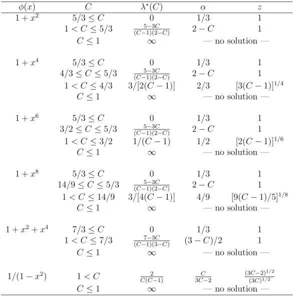
We take X = [−1, 1], Ψ(·) = log det(·) and consider several penalty functions φ(x), symmetric with respect to x = 0 where their reach their minimum value: φ(x) = 1 + x2q,
q = 1, 2, 3, 4; φ(x) = 1 + x2 + x4; φ(x) = 1/(1 − x2); the minimum cost φ∗ equals one for
each of them. For any λ, the optimal designs ξ∗ for (5) are symmetric with respect to 0
and take the form
ξ∗ = ½ −z 0 z 1−α 2 α 1−α2 ¾ , (10)
where the first row gives the support points and the second their respective weights. This gives det M(ξ∗) = α(1 − α)2z6. The D-optimal design ξ∗
D corresponds to z = 1 and α = 1/3.
For φ(x) = 1 + x2q, q integer, the optimal designs for problems P
1 and P2 correspond
to α = min{q/[3(q − 1)], 1/2} and z = min{[3/(2q − 3)]1/2q, 1} (note that z < 1 only for
q ≥ 4). The penalty functions φ(x) = 1 + x2+ x4 and φ(x) = 1/(1 − x2) respectively give
the optimal designs defined by (α = 3/5, z = 1) and (α = 5/9, z =p3/5). The optimal designs ξ∗ for P
3 obtained for the different φ(·) mentioned above are given
in Table 1, together with the optimal value λ∗(C) of the Lagrange coefficient associated
with C. When there is no solution, it means that λ∗(C) = ∞. When there is one, then
Φ(ξ∗) = C.
In order to check if the support points of ξ∗concentrate around x∗ = 0 when λ increases
(without computing ξ∗), we use (8) with the test designs ξλ = ξλ(γ) = ½ −γ 0 γ 1/3 1/3 1/3 ¾ . For φ(x) = 1 + x2q we get ∆(ξ
λ) = 2γ2q/3 and the condition (8) then gives ˆx2q ≤
[4γ2q/3] trace[µ(ˆx)M−1(ξ
λ)]. Noticing that trace[µ(γ t)M−1(ξλ)] = P (t) = 3(1 − 3/2t2 +
3/2t4) independently of γ (a property of D-optimal design for polynomial regression), we
obtain that a support point ˆx of ξ∗ must satisfy t2q ≤ 4P (t)/3, with t = |ˆx|/γ. For q = 3
we obtain t ≤ [1 + (1 + β1/3)2]1/2/β1/6 with β = 4 + 2√2, that is t . 2.2252. For q = 4, we
corresponds to α = 1 and ˜ξλ = ξλ in the proof of Proposition 1-(ii)). It gives |ˆx| ≤ ˆxmax
with ˆxmax' 2.860 λ−1/6 for q = 3 and ˆxmax=
√
2[9/(2λ)]1/8 ' 1.707 λ−1/8 for q = 4. This
is consistent with the rate of decrease of z in Table 1 when C tends to 1 (and λ∗(C) tends
to infinity). When q = 1, 2 all t are admissible and we cannot obtain a bound on |ˆx|; the
same situation occurs for the penalty function φ(x) = 1 + x2+ x4.
The case φ(x) = 1/(1 − x2) illustrates that it is the local behavior of φ(x) around the
minimum x∗ that influences the support of ξ∗ when λ tends to infinity. Indeed, 1/(1 − x2)
tends to infinity for x tending to ±1 but equals 1+x2+x4+O(x6) around x∗ = 0. Condition
(8) then becomes φ(γt) − φ(0) = γ2t2/(1 − γ2t2) ≤ 2 ∆(ξ
λ) P (t) = (4/3)γ2P (t)/(1 − γ2).
The bound obtained for t now depends on γ; the best bound (minimum) for |ˆx| is ˆxmax'
0.9649, obtained at γ ' 0.7385, and ∆(ξλ) ≥ p/λ imposes λ & 3.7516. Therefore, we only
learn from (8) that the support of ξ∗ is included in [−0.9649, 0.9649] for λ large enough.
This is consistent with the behavior of the support points −z, z of ξ∗ as λ tends to infinity,
which do not converge to zero (limλ→∞z = limC→1+z = 1/
√
3, see Table 1). ¤
3.3. Nonlinear cost-constrained design
In a nonlinear situation, like in the example presented in Sect. 4, where M(ξ, θ) and Φ(ξ, θ) depend on θ, robustness with respect to misspecifications of θ can be achieved by considering average-optimal design. Problem P3(θ) is then transformed into: maximize
IEθ{Ψ[M(ξ, θ)]} with respect to ξ ∈ Ξ under the constraint IEθ{Φ(ξ, θ)} ≤ C, where the
expectation IEθ is calculated for some prior probability measure ν for θ. For D-optimality,
the optimality condition (4) becomes
∃λ∗ ≥ 0 such that λ∗[C − IE θ{Φ(ξ∗, θ)}] = 0 and ∀x ∈ X , IEθ{trace[µ(x, θ)M−1(ξ∗, θ)]} ≤ p + λ∗IE θ{φ(x, θ) − Φ(ξ∗, θ)} .
Apart from additional numerical cost (which remains reasonable when ν is a discrete measure with a limited number of support points), the introduction of a prior probability for θ does not raise any special difficulty. This is used by Haines et al. (2003), with
φ(x, θ) = II[QR(θ),∞)(x), where IIA(x) is the indicator function of the set A (1 if x ∈ A,
0 otherwise) and QR(θ) is a quantile of the probability of toxicity, parameterized by θ, defining the maximum acceptable probability of toxicity (note that IEθ{φ(x, θ)} = ν{QR(θ) ≤ x}, the prior probability that x exceeds QR).
Another common approach to overcome the issue of dependence of the optimum design in θ consists in designing the experiment sequentially. In adaptive D-optimal design for instance, the design point after N observations is taken as
xN +1 = arg max
x∈X trace[µ(x, ˆθ
N)M−1(ξ
N, ˆθN)] , (11)
where ˆθN is the current estimated value of θ. By alternating between estimation based
φ(x) C λ∗(C) α z 1 + x2 5/3 ≤ C 0 1/3 1 1 < C ≤ 5/3 5−3C (C−1)(2−C) 2 − C 1 C ≤ 1 ∞ — no solution — 1 + x4 5/3 ≤ C 0 1/3 1 4/3 ≤ C ≤ 5/3 5−3C (C−1)(2−C) 2 − C 1 1 < C ≤ 4/3 3/[2(C − 1)] 2/3 [3(C − 1)]1/4 C ≤ 1 ∞ — no solution — 1 + x6 5/3 ≤ C 0 1/3 1 3/2 ≤ C ≤ 5/3 5−3C (C−1)(2−C) 2 − C 1 1 < C ≤ 3/2 1/(C − 1) 1/2 [2(C − 1)]1/6 C ≤ 1 ∞ — no solution — 1 + x8 5/3 ≤ C 0 1/3 1 14/9 ≤ C ≤ 5/3 5−3C (C−1)(2−C) 2 − C 1 1 < C ≤ 14/9 3/[4(C − 1)] 4/9 [9(C − 1)/5]1/8 C ≤ 1 ∞ — no solution — 1 + x2+ x4 7/3 ≤ C 0 1/3 1 1 < C ≤ 7/3 7−3C (C−1)(3−C) (3 − C)/2 1 C ≤ 1 ∞ — no solution — 1/(1 − x2) 1 < C 2 C(C−1) 3C−2C (3C−2)1/2 (3C)1/2 C ≤ 1 ∞ — no solution —
Table 1: Optimal designs ξ∗ for problem P
3 in Example 1, see (10). The optimal support points ±z
one forces the empirical design measure to progressively adapt to the correct (true) value of the model parameters. Adaptive design is considered in (Dragalin and Fedorov, 2006; Dragalin et al., 2008), but the convergence of the procedure (strong consistency of the parameter estimator and convergence of the empirical design measure to the optimal non-sequential design for the true value of the model parameters) is left as an open issue. The difficulty of proving the consistency of the estimator when design variables are sequentially determined is usually overcome by considering an initial experiment (non adaptive) that grows in size when the total number of observations increases, see, e.g., Chaudhuri and Mykland (1993). Although this number is often severely limited in prac-tise, especially for clinical trials, we think that it is reassuring to know that, for a given
initial experiment, adaptive design guarantees suitable asymptotic properties under
rea-sonable conditions. Using simple arguments, one can show that this is indeed the case when the design space is finite, which forms a rather natural assumption in the context of clinical trials. The case of adaptive D-optimal design is considered in (Pronzato, 2009b) (notice that is also covers the situation considered by Dragalin and Fedorov (2006); Dra-galin et al. (2008), which can be formulated as a standard D-optimal design problem).
In the case of adaptive penalized D-optimal design, the design point after N observa-tions is taken as xN +1= arg max x∈X n trace[µ(x, ˆθN)M−1(ξ N, ˆθN)] − λNφ(x, ˆθN) o . (12)
Following an approach similar to that in (Pronzato, 2009b), one can show that when X is finite, λN is the optimal Lagrange coefficient for problem P3(ˆθN), and under rather
standard regularity assumptions, this procedure is asymptotically “optimal” in the sense that the estimated value of the parameters (by least-squares in a nonlinear regression model or by maximum-likelihood in Bernoulli trials) converges a.s. to its true value ¯θ
and the information matrix tends a.s. to the penalized D-optimal matrix at ¯θ as N → ∞, see Pronzato (2009a). (Note that the true optimal design for sequential dependent
observations is extremely difficult to construct, see, e.g., Gautier and Pronzato (1998, 2000) for suboptimal attempts.) Moreover, the estimator is asymptotically normal, with variance-covariance matrix given by the inverse of the usual information matrix, similarly to the non-adaptive case, see Pronzato (2009a). The strong consistency of ˆθN is preserved
when λN is taken as a control parameter that tends to infinity not too fast (more slowly
than N/(log log N)). As in (Pronzato, 2000), by letting λN tend to infinity one focusses
more and more on cost minimization and thus obtain design measures that converge weakly to the delta measure at x∗ = arg min
x∈Xφ(x, ¯θ) (and when, moreover, the property
(9) is satisfied, all design points tend to concentrate around x∗).
As an illustration, an example with a nonlinear model with binary responses is con-sidered in the next section, first for local penalized optimal design and then for adaptive penalized optimal design through simulations.
4. Example: Cox model for efficacy-toxicity response
The example is taken from (Dragalin and Fedorov, 2006) and concerns a problem with bivariate binary responses. Let Y (respectively Z) denote the binary outcome indicating efficacy (resp. toxicity) for a trial at dose x. The set of available doses consists of 11 points equally spaced in the interval [−3, 3], X = {x(1), . . . , x(11)}, x(i) < x(i+1), i = 1, . . . , 10.
We write Prob{Y = y, Z = z|x, θ} = πyz(x, θ), Y, y, Z, z ∈ {0, 1}. The following
six-parameter model is used in (Dragalin and Fedorov, 2006) (we refer to that paper for motivations and justifications):
π11(x, θ) = ea11+b11x 1 + ea01+b01x+ ea10+b10x+ ea11+b11x π10(x, θ) = ea10+b10x 1 + ea01+b01x+ ea10+b10x+ ea11+b11x π01(x, θ) = ea01+b01x 1 + ea01+b01x+ ea10+b10x+ ea11+b11x π00(x, θ) = ¡ 1 + ea01+b01x+ ea10+b10x+ ea11+b11x¢−1
with θ = (a11, b11, a10, b10, a01, b01)>. The log-likelihood function of a single observation
(Y, Z) at dose x is then l(Y, Z, x; θ) = Y Z log π11(x, θ) + Y (1 − Z) log π10(x, θ) + (1 −
Y )Z log π01(x, θ) + (1 − Y )(1 − Z) log π00(x, θ) and elementary calculations show that the
contribution to the Fisher information matrix is
µ(x, θ) = ∂p >(x, θ) ∂θ ¡ P−1(x, θ) + [1 − π11(x, θ) − π10(x, θ) − π01(x, θ)]−111> ¢ ∂p(x, θ) ∂θ>
where p(x, θ) = [π11(x, θ), π10(x, θ), π01(x, θ)]>, P(x, θ) = diag{p(x, θ)} and 1 = (1, 1, 1)>.
Note that µ(x, θ) is generally of rank 3. As in (Dragalin and Fedorov, 2006), we take
θ = (3, 3, 4, 2, 0, 1)>. The D-optimal design is then supported on x(1), x(4), x(5) and x(10)
with respective weights 0.3318, 0.3721, 0.1259 and 0.1701.
Next section illustrates how a locally optimal design for (5) depends on the choice of
λ and φ.
4.1. Locally optimal design
We first choose a penalty function given by the inverse of the probability π10(x, θ) of
efficacy and no toxicity (probability of success) and take
φ1(x, θ) = π10−1(x, θ) .
The Optimal Safe Dose (OSD), maximizing π10(x, θ), is x(5) = −0.6. Figure 1 presents
the optimal designs ξ∗(λ) for λ varying between 0 and 100 along the horizontal axis. The
weight associated with each x(i) on the vertical axis is proportional to the thickness of
the plot. The design measure tends to give more and more weight to the OSD x(5) as λ
0 10 20 30 40 50 60 70 80 90 100 −3 −2 −1 0 1 2 3 λ ξ * {x (i) }
Figure 1: Optimal designs ξ∗(λ) as function of λ ∈ [0, 100] for the cost function π−1
10(x, θ): each horizontal
dotted line corresponds to a point in X , the thickness of the plot indicates the associated weight.
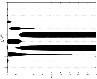
Consider now the cost function
φ2(x, θ) = {π10−1(x, θ) − [maxx π10(x, θ)]−1}2, (13)
also related to the probability of success, but more flat than π−1
10(x, θ) around its minimum
(at the OSD). Using the condition (8) with the test designs ξλ,1, giving weights (1−α)/2, α
and (1 − α)/2 at x(4), x(5) and x(6) respectively, and ξ
λ,2, giving weights 1 − β and β at x(4)
and x(5) respectively, we obtain that the support of ξ∗(λ) is included in {x(4), x(5), x(6)} for
α & 0.9993 and β & 0.4508, showing that the optimal designs concentrate on three doses
around the optimal one when λ is large enough. Figure 2 presents the optimal designs
ξ∗(λ) for λ varying between 0 and 100 along the horizontal axis. It shows that for λ & 75
the optimum designs are supported on x(4) and x(6) only, with weights approximately 1/2
each, that is, all patients in a trial defined by ξ∗(λ) receive a dose close to the optimal one, x(5). Note, however, that none receives the OSD (compare with Figure 2). The situations
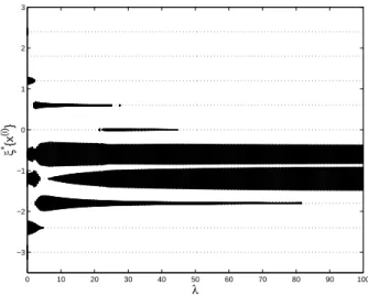
changes for larger values of λ, see Figure 3 where the optimal design is supported on
{x(4), x(5), x(6)} for λ & 160 and the weight of the optimal dose x(5) increases with λ.
Finally, one may also consider a penalty function that puts more stress on toxicity avoidance, for instance
φ3(x, θ) = π10−1(x, θ)[1 − π·1(x, θ)]−1, (14)
which is used in (Dragalin and Fedorov, 2006), with π·1(x, θ) = π01(x, θ) + π11(x, θ)
denot-ing the marginal probability of toxicity (the dose minimizdenot-ing φ3(x, θ) is then x(4)). For λ
large enough the optimal designs then tend to avoid large doses, compare Figure 4 with Figures 1 and 2.
4.2. Adaptive design
As an illustration of the behavior of the adaptive scheme (12), we present now some simulation results (using the value θ = (3, 3, 4, 2, 0, 2)>). For comparison, we use the
0 10 20 30 40 50 60 70 80 90 100 −3 −2 −1 0 1 2 3 λ ξ * {x (i) }
Figure 2: Same as Figure 1, but for the cost-function (13).
0 100 200 300 400 500 600 700 800 900 1000 −3 −2 −1 0 1 2 3 λ ξ * {x (i) }
Figure 3: Same as Figure 2, but for λ ∈ [0, 1000].
up-and-down rule of Ivanova (2003) (which is also considered by Dragalin and Fedorov (2006), see also (Kpamegan and Flournoy, 2001, p. 221)), defined by
xN +1= max{x(iN−1), x(1)} if Z N = 1 , x(iN) if Y N = 1 and ZN = 0 , min{x(iN+1), x(11)} if Y N = 0 and ZN = 0 , (15)
where the index iN ∈ {1, . . . , 11} is defined by x(iN) = xN and (YN, ZN) denotes the
observation for xN. The stationary allocation distribution ξu&d is log-concave and is
approximately given by ξu&d(θ) ' ½ x(1) x(2) x(3) x(4) x(5) x(6) x(7) x(8) 1.70 10−3 2.12 10−2 0.146 0.426 0.345 5.88 10−2 1.90 10−3 1.13 10−5 ¾
0 10 20 30 40 50 60 70 80 90 100 −3 −2 −1 0 1 2 3 λ ξ * {x (i) }
Figure 4: Same as Figure 1, but for the cost-function (14).
(the total weight on x(9), x(10), x(11) is less than 10−7). Note that the mode is at x(4), one
dose below the OSD x(5). See Durham and Flournoy (1994); Giovagnoli and Pintacuda
(1998); Ivanova (2003) for analytical results.
We consider trials on 36 patients, organized in a similar way as in (Dragalin and Fedorov, 2006): the allocation for the first 10 patients uses the up-and-down rule above, starting with the lowest dose x(1); after the 10th patient, the up-and-down rule is still used
until the first observed toxicity (ZN = 1); we then switch to the adaptive design rule (12),
with the restriction that we do not allow allocation at a dose one step higher than the maximum level tested so far (following recommendations for practical implementation, see Dragalin and Fedorov (2006)). The parameters are estimated by maximum likelihood (the log-likelihood Pil(Yi, Zi, xi; θ) being regularized by the addition of the term 0.01 kθk2,
which is equivalent to maximum a posteriori estimation with the normal prior N (0, 50 I), with I the 6-dimensional identity matrix).
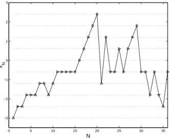
We first use the penalty function φ1(x, θ) = π−110(x, θ), with minimum value at the OSD
x(5), φ
1(x(5), θ) ' 1.2961. Figure 5 shows the progress of a typical trial with λN ≡ 2. The
symbols indicate the values of the observations at the given points: M for (Y = 0, Z = 0),
. for (Y = 1, Z = 0), ¦ for (Y = 1, Z = 1) and O for (Y = 0, Z = 1). The up-and-down
rule is used until N = 15 where toxicity is observed. The next dose should have been x(4)
but the adaptive design rule (12) selects x(6) instead.
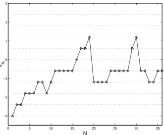
As noticed by a referee, in a practical implementation one would certainly be more cautious than what is shown on Figure 5: although toxicity is observed for subjects 17 and 19, the design recommends escalation to a higher dose. As shown on Figure 6, the substitution of the penalty function φ3(x, θ) given by (14) for φ1(x, θ) permits to avoid
this type of behavior (compare with Figure 5).
We now perform 1,000 independent repetitions of similar trials, using three differ-ent adaptive rules: (i) the up-and-down rule (15) used along the whole trial, for the 36 patients; (ii) the up-and-down rule followed by adaptive D-optimal design (11); and
0 5 10 15 20 25 30 35 −3 −2 −1 0 1 2 3 N x N
Figure 5: Graphical presentation of a trial with φ1(x, θ) = π10−1(x, θ) and λN ≡ 2 in (12); M is for
(Y = 0, Z = 0), . for (Y = 1, Z = 0), ¦ for (Y = 1, Z = 1) and O for (Y = 0, Z = 1).
(iii) the up-and-down rule followed by adaptive penalized D-optimal design (12), with
φ1(x, θ) = π10−1(x, θ) and λN ≡ 2. Since the choice λN ≡ 2 may seem arbitrary, we also
considered the situation (iv) where λN is adapted to the estimated value of θ. To
re-duce the computational cost, we only adapt λN once in the trial, at the value Ns when
we abandon the up-and-down rule. The value λN = λ∗Ns, N = Ns, . . . , 36, is chosen as
the solution for λ of Φ[ξ∗(λ), ˆθNs
M L] = Cγ = (1 + γ) minx∈Xφ(x, ˆθM LNs ); we take γ = 0.52
because it yields λ = 2 when θ is substituted for ˆθNs
M L, that is, Φ[ξ∗(2), θ]/φ∗θ ' 1.52 (it
corresponds to allowing an average reduction of about 34% for the probability of success compared to maxx∈Xπ10(x, ˆθNM Ls )). The solution for λ is easily obtained by dichotomy,
since we know that the solution satisfies 0 < λ ≤ (1 + 1/γ) p/Cγ, see Proposition 1-(i),
and Φ[ξ∗(λ), θ] decreases when λ increases (note that this is more economical in terms
of computations than the Lagrangian approach proposed in Sect. 2.3 of Cook and Fe-dorov (1995) in a more general situation). Table 2 summarizes the results in terms of the following performance measures: Φ1(ξ36, θ) = (1/36)
P36
i=1φ1(xi, θ), the total cost of
the experiment; J(ξ36, θ) = det−1/6[M(ξ36, θ)], which indicates the precision of the
esti-mation of θ; bx∗
{t=i}, the number of times the estimated OSD at the end of the trial, that
is, arg maxx∈Xπ10(x, ˆθ36M L), coincided with x(i), for i = 4, 5, 6, and bx∗{t<4} (resp. bx∗{t>6}),
the number of times the estimated OSD was smaller than x(4) (resp. larger than x(6));
finally #x(11), the percentage of patients that received the highest dose x(11). The values
of Φ1(ξ, θ) and J(ξ, θ) for the designs ξu&d, ξD∗ and ξ∗(λ = 2) computed at the true value
of θ are also indicated.
Table 2 reveals that the up-and-down rule (15) is very cautious: its associated cost Φ1(ξ36, θ) is low, the extreme dose x(11) has never been used over the 1,000 repetitions.
One the other hand, it fails at providing a precise estimation of the model parameters, and the OSD is estimated at values higher than x(6) in almost 14% of the cases. Parameter
0 5 10 15 20 25 30 35 −3 −2 −1 0 1 2 3 N x N
Figure 6: Graphical presentation of a trial, in the same conditions as in Figure 5 but with the penalty
φ3(x, θ) given by (14). design rule Φ1(ξ, θ) J(ξ, θ) xc∗{t<4} cx∗{t=4} xc∗{t=5} xc∗{t=6} xc∗{t>6} #x(11) (i): (15) 1.87 28.02 20 386 369 86 139 0 ξu&d(θ) 1.47 29.4 (ii): (15)–(11) 3.16 17.23 0 198 705 78 19 5% ξ∗ D(θ) 4.45 14.99 (iii): (15)–(12), φ1, λN≡ 2 2.25 19.22 3 231 693 59 14 1.6% ξ∗(λ = 2, θ), φ 1 1.97 17.00 (iv): (15)–(12), φ1, λ∗N 2.38 18.78 0 223 682 70 25 2.3% (v): (15)–(12), φ3, λN≡ 2 2.09 21.08 4 330 575 61 23 0.5%
Table 2: Performance measures of different adaptive designs for 36 patients (sample mean over 1,000 repetitions for Φ1(ξ) =
R
Xφ1(x, θ) ξ(dx) and J(ξ, θ) = det
−1/6[M(ξ, θ)]; cx∗A is the number of times
arg maxx∈Xπ10(x, ˆθ36M L) ∈ A and #x(11) is the percentage of patients that received the highest dose x(11) over the 1,000 repetitions). The values of Φ
1(ξ, θ) and J(ξ, θ) for ξu&d, ξD∗ and ξ∗(λ = 2) are also
indicated. In (iii) and (iv), the adaptive rule (12) uses the penalty function φ1(x, θ) = π10−1(x, θ), (v) uses
the penalty φ3(x, θ) given by (14).
x(5) is recognized in more than 70% of the cases. However, this successful behavior
in terms of collective ethics is obtained at the price of having about 5% of patients receiving a dose as high as x(11); also, the associated value of Φ
1(ξ36, θ) is rather high.
The adaptive penalized D-optimal design appears to make a good compromise between the two strategies: the value of Φ1(ξ36, θ) is close to that of the up-and-down rule, the
value of det−1/6[M(ξ36, θ)] is close to that obtained for adaptive D-optimal design. It
recognized x(5) as the OSD in about 70% of the cases and only 1.6% of the patients
received the dose x(11) when λ
N ≡ 2 (2.3% when λN is adapted). Of course, other choices
of λ would set other compromises. Also, other penalty functions can be used to define design rules more reluctant at allocating high doses: the performance of the adaptive penalized D-optimal design with the penalty (14) is indicated on line (v) of the table; comparison with line (iii) shows that the less precise estimation of the OSD is balanced by a more cautious strategy (only 0.5% of the patients receive the highest dose x(11)).
In order to limit more severely the number of patients that receive very high doses, we finally consider a compromise strategy that implements a smoother (and less arbitrary) transition between up-and-down and adaptive penalized D-optimal design.
Letting λN increase with N in (12) might be controversial in the context of
clini-cal trials (as mentioned by a referee, it implies a loss of randomization feature in the trial and brings potential for operational bias, not to mention the difficulties induced concerning the statistical analysis of the data accumulated during the trial due to the nonhomogeneous treatments at the beginning and the end of the trial). Thus, letting
λN depend on N might not be a realistic practical situation in this context. It is
in-structive, however, to investigate though simulations the performance achieved by such “non-stationary” designs. We thus consider much longer trials, with NT = 240 patients
enroled. Define x∗∗(θ) = arg min
x∈Rφ(x, θ) and h(x, θ) = ∂φ(x, θ)/∂x. From the implicit
function theorem, ∇θx∗∗(θ) = dx∗∗(θ) dθ = − · ∂h(x, θ) ∂x |x=x∗∗(θ) ¸−1 ∂h(x, θ) ∂θ |x=x∗∗(θ)
and, when using the up-and-down rule (15) the estimator ˆθN
M L asymptotically satisfies √
NVN−1/2[x∗∗(ˆθM LN ) − x∗∗(¯θ)]→ z ∼ N (0, 1) , N → ∞ ,d
where VN = [∇θx∗∗(ˆθM LN )]>M−1(ξN, ˆθM LN )[∇θx∗∗(ˆθM LN )]. Based on that, we decide to
switch from the up-and-down rule to the adaptive one when pVN/N < x(2) − x(1), the
interval between two consecutive doses. If Ns is the index of the patient for which the rule
changes, we take λNs as the solution for λ of Φ[ξ∗(λ), ˆθ
Ns
M L] = Cγ = (1+γ) minx∈Xφ(x, ˆθNM Ls )
with γ = 0.5 (thus targeting 33% of decrease with respect to the maximum of π10(x, ˆθNM Ls )).
The value of λNT at the end of the trial is chosen as the solution for λ of the same equation
with γ = 0.1 (allowing only 9% of decrease with respect to the maximum of π10(x, ˆθNM Ls )).
In between λN increases at a logarithmic rate, that is, λN = λNs[1 + a log(N/Ns)],
N = Ns, . . . , NT, with a = (λNT/λNs− 1)/ log(NT/Ns). When uncertainty on the OSD is
large, that is whenpVN/N > [x(2)− x(1)]/2, we also restrict the allocations at high doses
by adapting the design space, taken as XN = {x(1), . . . , x(iN)} at step N: the maximum
dose x(iN) allowed in (12) is never more than one step higher than previous dose and is
smaller than previous dose if toxicity was observed.
The results obtained for 150 repetitions of the experiment are summarized in Table 3 (the results obtained when the up-and-down rule (15) is used for the 240 patients are also indicated). One may notice the precise estimation of the OSD for the adaptive penalized design compared to the down rule (it even does slightly better than the up-and-down rule both in terms of Φ1(ξ, θ) and det−1/6[M(ξ, θ)]). At the same time, only about
0.11% of the patients received the maximal dose x(11).
5. Conclusions
We have shown that constrained optimal design can be formulated in a way that allows a clear balance between gaining information and minimizing a cost. A dose-finding
Φ1(ξ, θ) J(ξ, θ) cx∗{t<4} cx∗{t=4} xc∗{t=5} cx∗{t=6} cx∗{t>6} #x(11)
(15) 1.54 29.04 0 21 116 11 2 0
(15)–(12), φ1, λN % 1.52 27.87 0 13 135 1 1 0.11%
Table 3: Performance measures of adaptive design (12) with increasing λN for 240 patients (sample mean
over 150 repetitions for Φ1(ξ) =
R
Xφ1(x, θ) ξ(dx) and J(ξ, θ) = det
−1/6[M(ξ, θ)]; cx∗
A is the number of
times arg maxx∈Xπ10(x, ˆθ200M L) ∈ A and #x(11)is the percentage of patients that received the highest dose x(11) over the 150 repetitions). The adaptive rule (12) uses the penalty function φ
1(x, θ) = π10−1(x, θ).
example with bivariate binary responses has illustrated the potential of adaptive penalized
D-optimal design to set compromises between individual ethics (cost of the experiment,
related to the probability of success through the penalty function) and collective ethics (information gained from the trial, to be used for future patients). Further developments and numerical studies are required to define suitable rules for selecting cost functions and for choosing the value (or the sequence of values) for the penalty coefficients λN.
Appendix
Proof of Proposition 1.
(i) Since ξ∗ is optimal, we have for all x ∈ X : trace[µ(x, θ)M−1(ξ∗, θ)] ≤ p + λ [φ(x, θ) − Φ(ξ∗, θ)], see (4). This is true in particular at a x∗ defined by (6) and
trace[µ(x∗, θ)M−1(ξ∗, θ)] ≥ 0 gives the result.
(ii) For any a > 0, take λ ≥ a/∆θ(ξ) and define ˜ξ = (1 − α)ξ + αδx∗ with δx∗ the delta
measure at a point x∗ satisfying (6) and α = 1−a/[λ∆
θ(ξ)]. This gives Φ(˜ξ, θ)−φ∗θ = a/λ
and log det M(˜ξ, θ) ≥ p log(1 − α) + log det M(ξ, θ). Therefore,
log det M(ξ∗, θ) − λ[Φ(ξ∗, θ) − φ∗θ] ≥ log det M(˜ξ, θ) − λ[Φ(˜ξ, θ) − φ∗θ]
≥ p log a − a − p log ∆θ(ξ) + log det M(ξ, θ) − p log λ . (16)
Since Φ(ξ∗, θ) ≥ φ∗
θ, the result follows.
When φ(x, θ) is bounded by ¯φθ, the optimality of ξ∗ implies that for all x ∈ X ,
trace[µ(x, θ)M−1(ξ∗, θ)] ≤ B = p+λ ( ¯φ
θ−φ∗θ). Write µ(x, θ) = F>θ(x)Fθ(x) with F>θ(x) =
[f1,θ(x), . . . , fm,θ(x)] and fi,θ(x) a p-dimensional vector, i = 1, . . . , m. From the inequality
trace[µ(x, θ)M−1(ξ∗, θ)] ≤ B we obtain that f>
i,θ(x)M−1(ξ∗, θ)fi,θ(x) ≤ B, i = 1, . . . , m.
We have
Λmin[M(ξ∗, θ)] = Λ−1max[M−1(ξ∗, θ)] = [ maxkuk=1u>M−1(ξ∗, θ)u]−1.
Consider the optimization problem defined by: maximize u>A>Au with respect to A
and u respectively in Rn×p and Rp, n ≤ p, subject to the constraints kuk = 1 and
f>
i,θ(x)A>Afi,θ(x) ≤ B, ∀x ∈ X and ∀i = 1, . . . , m. The optimal solution is obtained for
A = v>∈ Rp such that |f>
i,θ(x)v| ≤ √
B, ∀x ∈ X , ∀i = 1, . . . , m, and b = v>v is maximal.
For x varying in X the fi,θ(x)’s span Rp (since a nonsingular information matrix exists).
Therefore, there exists a positive constant δ such that the optimal value for b is bounded by B/δ, and Λmin[M(ξ∗, θ)] > δ/B.
Proof of Proposition 2.
Since trace[µ(x, θ)M−1(ξ∗, θ)] ≤ p + λ [φ(x, θ) − Φ(ξ∗, θ)] for all x ∈ X when ξ∗ is
optimal, and RX {trace[µ(x, θ)M−1(ξ∗, θ)] − λφ(x, θ)} ξ∗(dx) = p − λ Φ(ξ∗, θ), we have
trace[µ(ˆx, θ)M−1(ξ∗, θ)] = p + λ [φ(ˆx, θ) − Φ(ξ∗, θ)] at any ˆx support point of ξ∗. Suppose
that λ is large enough so that there exists a design ξλ ∈ Ξ satisfying ∆θ(ξλ) ≥ p/λ.
We proceed as for Proposition 1-(ii) and construct a design ˜ξλ = (1 − α)ξλ + αδx∗ with
α = 1−p/[λ∆θ(ξλ)] so that Φ(˜ξλ, θ)−φ∗θ = p/λ. With the same notation as in the proof of
Proposition 1-(ii), we can write trace[µ(ˆx, θ)M−1(˜ξ
λ, θ)] =
Pm
i=1fi,θ>(ˆx)M−1(˜ξλ, θ)fi,θ(ˆx).
We then follow the same approach as in Harman and Pronzato (2007) and define H(ξ∗, ξ, θ) = M1/2(ξ∗, θ)M−1(ξ, θ)M1/2(ξ∗, θ) . We obtain trace[µ(ˆx, θ)M−1(˜ξ λ, θ)] = m X i=1 f> i,θ(ˆx)M−1/2(ξ∗, θ) H(ξ∗, ˜ξλ, θ)M−1/2(ξ∗, θ)fi,θ(ˆx) ≥ Λmin[H(ξ∗, ˜ξλ, θ)] trace[µ(ˆx, θ)M−1(ξ∗, θ)] = Λmin[H(ξ∗, ˜ξλ, θ)] {p + λ [φ(ˆx, θ) − Φ(ξ∗, θ)]} ≥ Λmin[H(ξ∗, ˜ξλ, θ)] n p + λ [φ(ˆx, θ) − Φ(˜ξλ, θ)] o = Λmin[H(ξ∗, ˜ξλ, θ)] λ [φ(ˆx, θ) − φ∗θ]
where we used the property ∆θ(ξ∗) ≤ p/λ = ∆θ(˜ξλ), see (i). Therefore,
trace[µ(ˆx, θ)M−1(ξ λ, θ)] ≥ (1 − α)trace[µ(ˆx, θ)M−1(˜ξλ, θ)] (17) ≥ p Λmin[H(ξ ∗, ˜ξ λ, θ)] [φ(ˆx, θ) − φ∗θ] ∆θ(ξλ) . (18)
The last step consists in deriving a lower bound on Λmin[H(ξ∗, ˜ξλ, θ)] that does not depend
on ξ∗. Since tracehH−1(ξ∗, ˜ξ λ, θ) i =RX trace [µ(x, θ)M−1(ξ∗, θ)] ˜ξ λ(dx), the optimality of ξ∗ implies trace h H−1(ξ∗, ˜ξλ, θ) i ≤ p + λ Z X [φ(x, θ) − Φ(ξ∗, θ)] ˜ξλ(dx) = p + λ hΦ(˜ξλ, θ) − Φ(ξ∗, θ) i ≤ p + λ h Φ(˜ξλ, θ) − φ∗θ i = 2p . (19)
Therefore, Λmin[H(ξ∗, ˜ξλ, θ)] ≥ 1/(2p), which, together with (18), concludes the proof.
One might notice that, following Harman and Pronzato (2007), a tighter bound could be obtained in (8) by using trace[H(ξ∗, ˜ξλ, θ)] ≤ max x∈X[µ(x, θ)M −1(˜ξ λ, θ)] ≤ (1 − α)−1 max x∈X[µ(x, θ)M −1(ξ λ, θ)]
in addition to (19). However, since (1 − α)−1 = λ∆
θ(ξλ)/p, the improvement obtained for
Acknowledgements. The author wishes to thank V. Fedorov for his comments and N.
Flournoy for her careful reading of the paper, her detailed comments and advice. The careful reading of the two referees is gratefully acknowledged.
References
Chaudhuri, P., Mykland, P., 1993. Nonlinear experiments: optimal design and inference based likelihood. Journal of the American Statistical Association 88 (422), 538–546. Cook, D., Fedorov, V., 1995. Constrained optimization of experimental design (invited
discussion paper). Statistics 26, 129–178.
Cook, D., Wong, W., 1994. On the equivalence between constrained and compound opti-mal designs. Journal of the American Statistical Association 89 (426), 687–692.
Dragalin, V., Fedorov, V., 2006. Adaptive designs for dose-finding based on efficacy-toxicity response. Journal of Statistical Planning and Inference 136, 1800–1823.
Dragalin, V., Fedorov, V., Wu, Y., 2008. Adaptive designs for selecting drug combinations based on efficacy-toxicity response. Journal of Statistical Planning and Inference 138, 352–373.
Durham, S., Flournoy, N., 1994. Random walks for quantile estimation. In: Berger, J., Gupta, S. (Eds.), Statistical Decision Theory and Related Topics V. Springer, New York, pp. 467–476.
Fedorov, V., Hackl, P., 1997. Model-Oriented Design of Experiments. Springer, Berlin. Gautier, R., Pronzato, L., 1998. Sequential design and active control. In: Flournoy, N.,
Rosenberger, W., Wong, W. (Eds.), New Developments and Applications in Experimen-tal Design, Lecture Notes — Monograph Series, vol. 34. IMS, Hayward, pp. 138–151. Gautier, R., Pronzato, L., 2000. Adaptive control for sequential design. Discussiones
Mathematicae, Probability & Statistics 20 (1), 97–114.
Giovagnoli, A., Pintacuda, N., 1998. Properties of frequency distributions induced by general ‘up-and-down’ methods for estimating quantiles. Journal of Statistical Planning and Inference 74, 51–63.
Haines, L., Perevozskaya, I., Rosenberger, W., 2003. Bayesian optimal designs in Phase I clinical trials. Biometrics 59, 591–600.
Hardwick, J., Stout, Q., 2001. Optimizing a unimodal response function for binary vari-ables. In: Atkinson, A., Bogacka, B., Zhigljavsky, A. (Eds.), Optimum Design 2000. Kluwer, Dordrecht, Ch. 18, pp. 195–210.
Harman, R., Pronzato, L., 2007. Improvements on removing non-optimal support points in D-optimum design algorithms. Statistics & Probability Letters 77, 90–94.
Ivanova, A., 2003. A new dose-finding design for bivariate outcomes. Biometrics 59, 1001– 1007.
Kiefer, J., Wolfowitz, J., 1960. The equivalence of two extremum problems. Canadian Journal of Mathematics 12, 363–366.
Kpamegan, E., Flournoy, N., 2001. An optimizing up-and-down design. In: Atkinson, A., Bogacka, B., Zhigljavsky, A. (Eds.), Optimum Design 2000. Kluwer, Dordrecht, Ch. 19, pp. 211–224.
Mikuleck´a, J., 1983. On a hybrid experimental design. Kybernetika 19 (1), 1–14.
Pronzato, L., 2000. Adaptive optimisation and D-optimum experimental design. Annals of Statistics 28 (6), 1743–1761.
Pronzato, L., 2009a. Asymptotic properties of nonlinear least squares estimates in stochas-tic regression models over a finite design space. Application to self-tuning optimisation. In: Proc. 15th IFAC Symposium on System Identification, Saint-Malo, France.
Pronzato, L., 2009b. One-step ahead adaptive D-optimal design on a finite design space is asymptotically optimal. Metrika (to appear).
![Figure 1: Optimal designs ξ ∗ (λ) as function of λ ∈ [0, 100] for the cost function π 10 −1 (x, θ): each horizontal dotted line corresponds to a point in X , the thickness of the plot indicates the associated weight.](https://thumb-eu.123doks.com/thumbv2/123doknet/13533230.418011/14.892.282.615.162.432/optimal-function-function-horizontal-corresponds-thickness-indicates-associated.webp)